Article

The Use of TOPSIS Method for Multi-Objective Optimization in Milling Ti-MMC

by
Saeid Kamalizadeh
1,
Seyed Ali Niknam
1,2,*,
Marek Balazinski
1 and
Sylvain Turenne
1,*
1
Mechanical Engineering Department, Polytechnique Montreal, Montréal, QC H3T 1J4, Canada
2
Sustainable Manufacturing Systems Research Laboratory, School of Mechanical Engineering, Iran University of Science and Technology, Tehran 13114-16846, Iran
*
Authors to whom correspondence should be addressed.
Metals 2022, 12(11), 1796; https://doi.org/10.3390/met12111796
Submission received: 30 August 2022 / Revised: 3 October 2022 / Accepted: 19 October 2022 / Published: 24 October 2022

Abstract

:
This paper presents the use of TOPSIS, a multi-criteria decision-making model combined with the Taguchi method to find the optimum milling parameters. TOPSIS is the Technique for Order Preference by Similarity to the Ideal Solution and shows the value of closeness to the positive ideal solution. This study shows the optimum combination of process parameters using the shortest distance from the ideal solution. The surface roughness and flank tool wear were considered the objectives for simultaneous optimization. After converting multiple responses into a single response, the Taguchi method was used to analyze and determine the optimum machining parameters. According to reported studies, the initial wear behavior and initial cutting conditions have significant effects on the tool wear progress. Several initial cutting parameters can contribute to tool life and therefore can be used to improve both tool life and surface roughness. However, the cutting speed may significantly affect tool wear and ultimate tool life. In this study, an innovative solution was proposed for interrupted machining with two different cutting speeds. The first level cutting speed was used for 1 s and the second level was used for the rest of the process. The experimental results indicate that the initial speed followed by the feed rate significantly affects tool life. In addition, using the proposed strategy with different levels of cutting speed during machining operations led to improved tool life and surface roughness compared to conventional machining with uniform cutting speed throughout the entire process.

1. Introduction

1.1. Background

Numerous studies and publications were reported on optimizing the cutting parameters and proposing the model for the relationship between cutting parameters and responses. Garg et al. [1] developed an empirical model that optimized machining parameters to minimize power consumption. They also studied the influence of machining parameters on energy consumption and their model reduced the power consumption of machine tools. Kant and Sangwan [2,3] developed a predictive and optimization model to predict the optimal value of machining parameters and minimize surface roughness. Their model was capable of determining the optimum machining parameters. Pusavec et al. [4] also studied the effects of the cutting process as inputs on the cutting forces, surface roughness, and tool wear. They also provided a chip breakability model in machining high-temperature Inconel 718. Their results showed a significant improvement in the machining process by optimizing parameters combined with sustainable alternative cooling and lubrication conditions.
Furthermore, several researchers have optimized cutting criteria, such as cutting forces, power consumption, surface roughness, and tool life. However, finding the optimal cutting parameters for certain objectives or responses requires machining knowledge and an adequate understanding of the relationship between the input parameters and the responses [5]. Although single-objective optimization has been broadly used, it has a major limitation when used in machining. It shows the optimum cutting parameters for a particular response and ignores the other objectives. However, unlike a single objective, in the multi-objective optimization method, all important objectives are simultaneously targeted by finding the optimum value of the input factors. Hence, a multi-objective method is more accurate and practical for this study. In 2016, Bilga et al. [6] reported the single-objective optimization of energy consumption for turning EN 353 alloy steel using the Taguchi method with Analysis of Variance (ANOVA). They optimized the cutting parameters individually for each response. The results show different optimum values in each case. One year later, Kumar et al. [7] repeated the similar work reported in [6] but for multi-response optimization, and optimized six responses using TOPSIS (Technique for Order Preference by Similarity to Ideal Solution). This approach was introduced by Hwang and Yoon in 1981 [8] to find the best alternatives with the shortest separation from the positive ideal solution and farthest distance from the perfect negative solution. The method is thoroughly discussed in Section 4.
Multi-criteria decision making (MCDM) is a method that evaluates and addresses decision issues by combining the effects of each criterion for multiple decision criteria, resulting in an optimal solution. The application of MCDM methods in machining process improvement has steadily increased. In the literature [9], three main groups of MCDM methods are:
  • Full aggregation methods, such as the analytic hierarchy process (AHP). This method assigns a weight to each criterion to show its importance. Then, the value of each alternative is determined and the highest positive value shows the best fit. The drawback is the complexity and time-consuming process depending on the inputs’ numbers.
  • Outranking methods, such as the ELimination Et Choix Traduisant la REalité (ELECTRE). In this method, to rank the alternatives, each pair of alternatives is compared for each criterion. The drawback is that this method needs several technical parameters, which are sometimes complex and hard to understand.
  • Goal, aspiration, or reference level methods, such as the TOPSIS method. The most significant advantage of this method is that it needs only a few inputs and its output is easy to understand. This makes the process pretty straightforward and comprehensible. This is the main reason for using TOPSIS for this study.
The responses found in [7] were power consumption, power factor, surface roughness, material removal rate, energy efficiency, and active energy consumption. Rao et al. [10] focused on the parametric optimization of cutting speed, federate, and cut depth in turning AA 6351 alloy using carbide tool. Their objective was to maximize the machining rate while minimizing surface roughness using the TOPSIS method. Their results showed a significant improvement for the responses. They found that the major process parameter affecting the multi-responses is cutting speed with a contribution of 38.68%. The contribution of feed rate was 34.51% and the depth of cut contribution was 21.91%. Mandal et al. [11] conducted several experiments to optimize electro-discharge machining using MOPSO_TOPSIS with four controlling components. They adopted Taguchi L9 orthogonal array for the experiments and TOPSIS to find the most desirable controlling parameters.
The Taguchi method is one of the most popular and powerful methods to analyze machining parameters and to determine the best process control factors. One of the main advantages of this method over the other methods is that more quantitative results can be obtained by performing less experiments, which also reduces the amount of experimentation and, consequently, the experimental costs. Taguchi’s method is also pretty straightforward and easy to apply to the machining process. However, it is a single-response optimization method and is not a proper method for simultaneously optimizing several responses. The other drawback of this method is that the results are strongly dependent on and relative to the number of input parameters and do not test all variable combinations. Despite these disadvantages, Taguchi’s method is extremely useful for experimental design. Titanium-based metal matrix composites (Ti-MMCs) are relatively new materials for both industry and academia, and many uncertainties exist about the difficulties and restrictions in their production, formation, and machining. Therefore, an overview of the machinability attributes of MMCs is introduced in the following sections. High tool wear rate, short tool life, and poor surface quality are the main concerns in machining Ti-MMCs. Due to the very low thermal conductivity of Ti-MMCs, very high local temperatures are generated in a tiny area around the cutting edge, resulting in a high tool wear rate [12]. Indeed, flank wear is a major machining issue because of the hard and abrasive particles in Ti-MMCs. For the successful and high production of components made of Ti-MMCs, such as engine parts of airplanes or cars, sometimes having a suitable surface finish is more critical than machining costs. Theoretically, two factors can play the more important roles in surface roughness: feed rate and tool geometry [13]. However, the high affinity of almost all tool materials to Ti-MMC’s matrix, especially at elevated temperatures in the tool-workpiece engagement, leads to a chemical reaction, material diffusion, and adhesion in the cutting tool [14]. Consequently, even at a high material removal rate (MRR), the chips cannot evacuate the massive thermal loads [15]. Moreover, the tool mostly slides more than cuts the workpiece at a low shear angle; therefore, similar to friction, the cutting zone temperature and pressure increase [16]. Then, the scraped materials melt and adhere to the tooltip. The hot adhered particles in the vicinity of oxygen turn into fragments, including titanium oxide and vanadium oxide [17]. It is worth mentioning that there are many studies [18] showing that the type of tool and its noise ratio can impact the surface roughness. As a rule of thumb, when other factors, such as machining speed, work material, coolant, etc., are not taken into consideration, a larger noise radius results in better surface roughness. Liang et al. [19] studied the effect of the welding thermal treatment on the microstructure and mechanical properties of nickel-based superalloy fabricated by selective laser melting. Their results quantified the respective contributions of the four conventional strengthening mechanisms. Zhong et al. [20] studied the microstructure and mechanical properties in the lap weld. They found that the number of cracks in the lap joint positively correlates with the size of the Ti2Ni region of the brittle intermetallic compound.
Usually, tool life is identified based on a typical tool wear curve versus cutting time. This curve shows three regions: the primary or initial, the steady state, and the accelerated wear period. Most of the research studies focus on the steady-state zone, which is more practical for traditional materials. However, due to the short tool lifetime, the initial moments of machining become more critical when it comes to difficult-to-cut materials. In other words, except for limited studies, the effects of the first moment of machining on tool life and initial tool wear mechanism have not been clearly determined and this field is open to more investigation. Amongst reported works, Troung [21,22] performed several experimental studies on the initial tool wear in the machining of Ti-MMCs and investigated the effect of the initial tool wear and initial cutting conditions on tool wear progression and tool life. Furthermore, the sensitivity of tool life to the initial cutting conditions was studied. It was exhibited that initial cutting conditions, such as initial speed, feed rate, and depth of cut within the first tool wear period improved tool life while turning Ti-MMC. In addition, Troung [21,22] discovered a protective layer forming in the first stage of tool wear, which could influence tool life. This so-called brace shield is a protective layer for the steady wear region. The formation of the brace shield provides a better explanation for the tool wear rate during the first wear period due to the accelerated cutting force and temperature concentrated in a tiny area. Finally, he suggested a chaos theory to explain the formation mechanisms of wear-protective tribo-films. However, the formation mechanisms of the protective tribo-films are not yet fully understood due to the complex chemo-mechanical interactions at the contact region and the limited three-dimensional resolution of many typically used characterization methods. In 2019, Aramesh et al. [23] was granted a US patent on an ultra-soft cutting tool coating and coating method. The cutting tool contains a substrate with a cutting surface and an ultra-soft coating adhered to the cutting surface in a solid state. This soft metal can melt and work as an in-place liquid lubricant. Their method also provides a practical way of shaping a tribo-film between the workpiece and the cutting tool. In two different studies, Abdelali, Beste, and colleagues [24,25] showed that when machining starts in a very short period, the cutting forces increase drastically and, consequently, so does the friction between two new surfaces where the relative sliding speeds are close to zero. This leads to high stress in a small area at the tool–workpiece interface. This very rapid initial increase in the cutting forces, which results in an immediate increase in cutting temperature, happens within one second and is followed by a slow but constant rate of increase during the second wear period [26,27]. According to standard in machining Ti-MMCs, contact conditions, the interface between the tool and workpiece, and cutting temperatures are the most influential factors in the wear mechanisms [28]. In [28], with a speed of 90 m/min, feed rate 0.2 mm/rev, and depth of cut 0.15 mm, machining has the optimal conditions, meaning less tool wear and better surface roughness.
In contrast, Troung [29] found that at lower speeds, i.e., 50 m/min, tool wear is less than that at higher speeds. In addition, a new theory was presented to relate the initial moments of machining to the rest of the process. Still, some of the observations and conclusions made by the authors of [29], such as the initial wear mechanism, are dissimilar to observations made by Bejjani [28] and Aramesh [30]. Asgari et al. [31] observed that the carbide tools demonstrate an acceptable tool wear rate despite a bit of vibration during the milling of Ti-MMCs. Their study showed that the optimum machining parameters are: cutting speed (Vc) = 45 m/min, feed rate (f) = 0.2 mm/rev, and depth of cut (ap) = 0.16 mm for the X500 carbide tool, and Vc = 70 m/min, f = 0.35 mm/rev, and ap = 1.5 mm for the X400 carbide tool. Based on their results, cutting speed is the main factor influencing the tool wear rate for the PCD tool.
Finally, Kamalizadeh et al. [26] focused on initial tool wear in turning Ti-MMCs using carbide tools. It was observed that the first transition time within the tool wear curve occurs in the first second of machining. Furthermore, a favorable correlation was found between the transition time in tool wear progression charts and the cutting force diagrams. As noted in [26], the primary wear mechanism during the initial moments of machining Ti-MMC is abrasion and the dominant wear mechanism is adhesion. The literature allows us to state that few studies are available on Ti-MMCs, mainly when dealing with the milling of Ti-MMCs, which is more costly and complex than turning. Therefore, an adequate selection of optimal milling parameters has evolved.

1.2. Contribution of This Work

This paper presents a multi-objective optimization model to optimize the milling parameters in the milling process using the Technique for Order Preference by Similarity to the Ideal Solution (TOPSIS). The surface roughness and flank tool wear were considered simultaneous optimization objectives. To the best of the authors’ knowledge, the initial cutting speed and its effects on the tool wear morphology when machining Ti-MMC has not yet been studied and no work was observed by means of tool life improvement when changing cutting speed at initial moments of cutting operation. To that end, it was also noted that the use of the TOPSIS method in the machining of Ti-MMCs is relatively new as the authors did not find any study that used this model, neither for ranking machining parameters nor for multi-objective optimization of the machining process.
Experimental results confirm that the initial machining conditions significantly affect ultimate tool life. In addition, the significant effects of initial and secondary cutting speed on the tool wear progress and ultimate tool life were noticed. Moreover, the strategy of cutting with two different speeds, mainly the initial and the secondary cutting speed, reduced wear rate by 105.5% and surface roughness by 143.2% compared to readings made in traditional machining with a constant cutting speed. The structure of the paper is as follows: Experimental methodology is described in Section 2. Then, the results and the approach used to convert multi-response into single response using TOPSIS and determine optimal cutting parameters using the Taguchi method are presented in Section 3. The next section presents a discussion of the results. Finally, conclusions are presented in Section 5.

2. Materials and Methods

This study presents a multi-objective optimization model to optimize the machining parameters in milling Ti-MMCs using carbide inserts. Two surface roughness (Ra) and tool flank wear values were the main machinability attributes for optimization purposes. In addition, the initial cutting speed, secondary cutting speed, and feed rate were input parameters. TOPSIS is used to identify the optimal milling parameters. Furthermore, the Taguchi method was used to determine the optimum machining parameters after converting multiple responses into a single response. According to previous studies [22,26], the initial moments of machining and initial tool wear behavior significantly affected tool life. Hence, the initial condition strategies were applied for 1 s of machining. Furthermore, based on two studies performed in 2017 [26,29], this initial period was sufficient to see the positive value of a scattered wear exponent. However, these researchers also found that the wear rate at lower speeds is pretty constant during the steady wear period after only one second of machining time, especially when the protective layer, the so-called brace shield, is shaped.
Since not much data are available on proposed cutting process parameters for machining Ti-MMC, especially regarding the milling process, some main parameters governing other machinability attributes (in principle R a ) are unclear. Hence, the statistical tools and approaches were used in this study to assess the controllability of the R a and VB max under various cutting conditions.

Machining Tests

Dry milling tests were conducted on a three-axis milling machine (Mitsui Seiki, Franklyn lakes, NJ, USA). The experiment setup is shown in Figure 1. A cubic shape of Ti-6Al-4V alloy matrix reinforced with at 10–12% volume fraction of TiC ceramic particles was used in this study. The elemental composition of Ti-MMC is shown in Table 1.
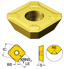
CoroMill 245 TiAlN + TiN nano-laminate Physical Vapor Deposition (PVD) coated carbide grades (Sandvik R245-12 T3 K-MM 2030) was utilized for this study, as shown in Table 2. These inserts can be used in the milling process of hard-to-cut alloys, such as Ti-MMCs, showing high levels of toughness and complex surface components, especially in the semi-finished process. In addition, a hard PVD deposited coating on the tool surface can decrease the abrasion wear mechanism and, at the same time, protect it from scratching and grooving by the work material’s tough TiC particles. Moreover, the difference between the price of TiAlN+TiN PVD-coated tools and other superior tools, such as CBNs or diamonds, makes this type of tool an excellent candidate for experimental studies. However, the machining process used in this study should not be very long due to the high cost of the Ti-MMC sample. This may gradually increase the experiment’s cost with less benefit.
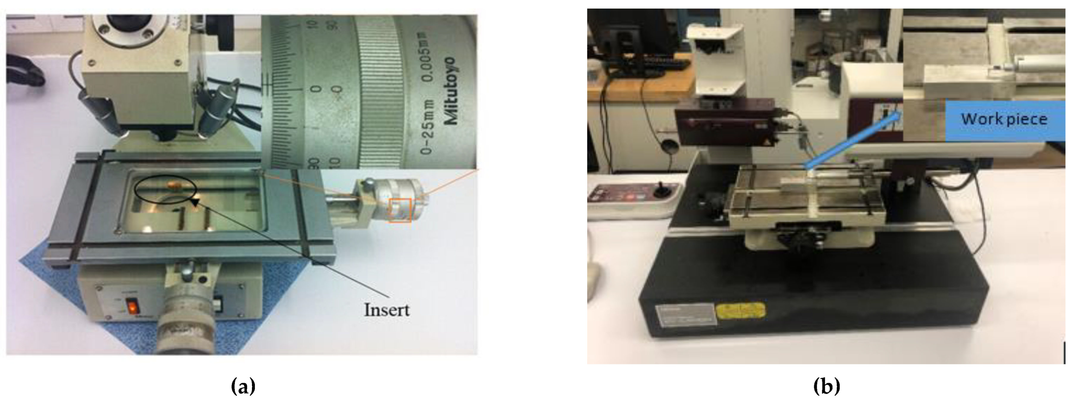
The work part surface roughness and tool flank wear were measured after each test using an optical microscope (Mitutoyo Corp., Tokyo, Japan) (Figure 2a) and a surface profilometer Mitutoyo SV-C4000 (Mitutoyo Corp., Tokyo, Japan) (Figure 2b).
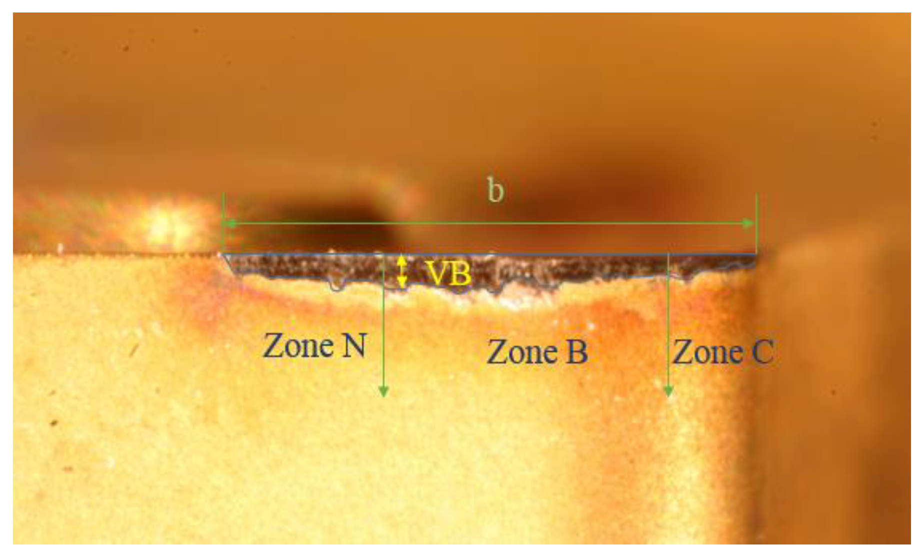
Tool wear was measured according to the ISO standard VB max as a common quantitative parameter. To measure VB max (Figure 3), the cutting tool worn-out length (b) was measured using a toolmaker optical microscope (Figure 2a) with a precise measurement of 0.005 mm. Then, near zone N (equal to b/4), the distance between the rake face and the end of the worn-out region, VB max, was measured. The arithmetical mean roughness value R a was used to characterize surface roughness (Figure 4). The smaller the R a , the smoother the machined surface.
For each insert, sequential milling tests were performed and VB max and R a were measured for each edge of the insert. In order to have very accurate results, each test was performed with a new and sharp edge of the insert, which amounted to a total of 4 tests for each insert. To avoid the effects of the previous cutting on the workpiece and tool elements, every new test was conducted using an unused edge of the insert. All tests were repeated two times to ensure that the tests were correctly carried out. For the surface roughness measurements, since our profilometer was placed in a temperature-controlled room and all measuring parameters are based on the ISO 4278 routine calibration procedure, these conditions guarantee the result accuracy.
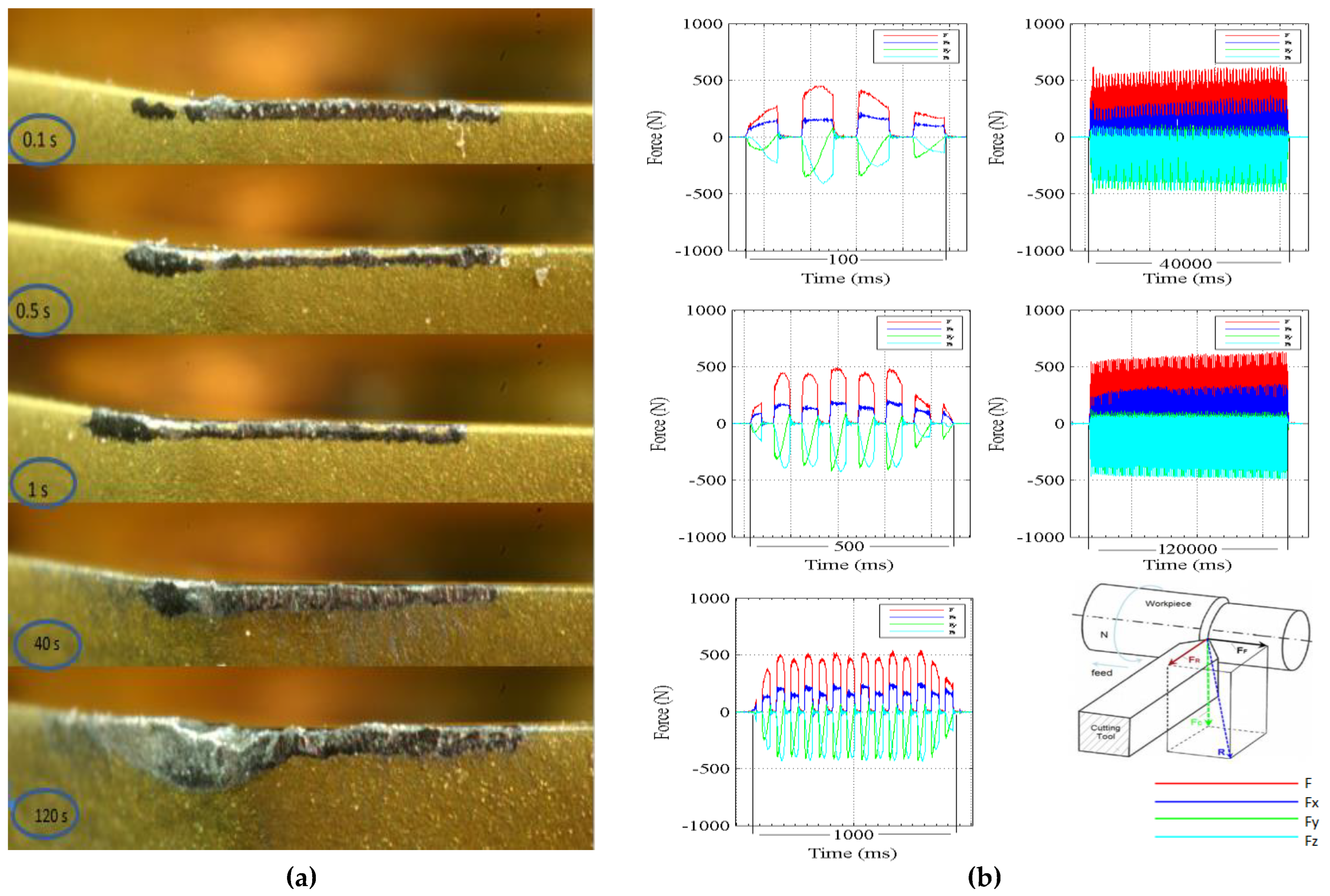
A Kistler dynamometer was used to monitor and record the cutting force signals in three directions related to the thrust force (FR), feed force (FF), and cutting force (FC), as depicted in Figure 5b. The sampling frequency of 10,000 Hz was used to analyze the cutting force signals. The cutting forces were analyzed in both time and frequency domains to evaluate the machining tests’ vibrational modes (chatter and forced) (Figure 5a). Minor tool vibration was observed in several tests, especially in those with higher levels of cutting speed (i.e., 80 m/min). However, despite vibration, the major difference in wear rate or surface roughness was not observed during the tests. No tool breakage was observed. Moreover, except in minor cases, an acceptable tool wear rate was observed in all cutting tests.

3. Results

3.1. Cutting Conditions and Experimental Results

According to previous studies, cutting speed and feed rate are the most crucial parameters in machining Ti-MMCs [21]. Therefore, in this study, to see the main effects of the initial cutting conditions on tool life, two different cutting speeds were used, including the initial speed for 1 s and the secondary cutting speed used in the rest of the machining operation. The constant cutting time of 120 s was selected based on previous studies [12]. According to preliminary investigations, it was found that severe tool wear occurs around this machining time, and flank tool wear passes 250 µm, which is considered a tool wear threshold.
Various feed rates were also considered based on industrial recommendations, machine tool capacity, and previous studies. The proposed levels of feed rates are tabulated in Table 3. According to the proposed cutting speeds and feed rate levels, the experiments were designed as an L27 full factorial orthogonal array (shown in Table 4). In addition, machining tests were conducted four times for each cutting condition to present a more accurate tool life curve and the average recorded values were considered for additional studies.
The cutting conditions were selected based on recommendations by the tool manufacturer. Machining tests were conducted several times for each cutting condition, and the average values of responses were used. This makes tool life curve more accurate. The statistical approach (i.e., TOPSIS and Taguchi) was used to define the factors governing flank wear of the inserts VB max and the surface roughness R a of the machined parts. Due to the lack of space and technical scope of the presenting work, no comprehensive overview of statistical tools (mostly the Taguchi method) and analysis procedures based on statistical tools is presented in this work.
Table 4 shows tool wear rates VB max (µm) and surface roughness R a (µm) under different cutting conditions. At certain level for the initial cutting speed V1, secondary cutting speed V2, and feed rate, the best conditions were obtained with acceptable productivity and cutting volume.

3.2. Conversion of Multiple Responses into a Single Response Using the TOPSIS Method

This study used the TOPSIS approach to convert multiple responses into one. Then, the Taguchi method was used to optimize the objectives. The TOPSIS approach was introduced by Hwang and Yoon [8] in 1981 to find the best alternatives with the shortest separation from the positive ideal solution and farthest distance from the negative ideal solution. The following steps are commonly applied to transfer the multiple responses into a single response [33]:
Step 1:
In the first step, the experimental decision matrix ( a i j ), which is usually called an “evaluation matrix” was created. In this matrix, each row (i) represents the alternative (experimental run number) and each column (j) represents the criteria (responses).
a i j = [ a 11 a 12 a 1 j a 1 m a 21 a 22 a 2 j   a 2 m a i 1 a i 2 a i j   a i m     a n 1 a n 2 a n j a n m   ]
For our case, in this matrix, i is the number of experiments that is 27 and j is the number of responses that is equal to two R a and VB max. The experimental values listed in Table 4 were used for the experimental decision matrix a ij elements as mentioned earlier in Equation (1). All the calculations are also rounded up to four digits after the decimal.
Step 2:
In this step, the evaluation matrix was normalized. Therefore, the responses were normalized for a limit of 0–1. This is to place them on a simple scale and remove the variation in their measuring units. The higher its value, the better the metric. The following equation was used to obtain the normalized matrix αij and all of the values are listed in Table 5.
α ij = a i j i = 1 n ( a i j ) 2
Step 3:
Next, the weighted normalized decision matrix ( x i j ) was calculated by multiplying each normalized metric from Step 2 by the assigned weight of their respective response (wj). It should be noted that each criterion must have its weight, all of which sum up to one.
x i j = [   w j   α i j ]
Both performance characteristics (responses) are considered equally important in this case. Hence, for each response, the relative weight of 0.5 is given and, using Equation (3), the weighted normalized matrix x i j is calculated, which is shown in Table 5.
Step 4:
In this step, the ideal positive (best) ( x j b ) and ideal negative (worst) ( x j w ) alternative for each criterion (response) were gained by using Equations (4) and (5). The idea is to find the maximum and minimum value of each metric. In all cases, surface roughness and flank tool wear are best when at a minimum, meaning that the smallest is the best.
x j b = { i m a x x i j / j   L ,   i m i n x i j / j   L ,   i = 1 ,   2 ,   3 ,     . ,   27   }
x j w = { i m i n x i j / j   L ,   i m a x x i j / j   L ,   i = 1 ,   2 ,   3 ,     . ,   27   }
In these equations, L (l = 1, 2, 3, …, 27) │ l was linked to beneficial characteristics or positive impact. L′ (l = 1, 2, 3, …, 27) │ l was linked to non-beneficial characteristics or negative impact. In this work, the values of ( x j b ) and ( x j w ) for surface roughness are 0.0386 and 0.1579, respectively, whereas ( x j b ) and ( x j w ) for flank tool wear are 0.0377 and 0.1498, respectively.
Step 5:
In this step, the Euclidean geometric distance between the target alternative and the best and worst alternatives ( d i b , d i w ) was calculated amongst all for the ideal positive ( x j b ) and ideal negative ( x j w ) using Equations (6) and (7).
d i b = j = 1 N ( x i j x j b ) 2
d i w = j = 1 N ( x i j x j w ) 2
In our case:
d i b = j = 1 27 ( x i j x j b ) 2
d i w = j = 1 27 ( x i j x j w ) 2
In Table 6, the values of separation ( d i b ) and ( d i w ) are shown. The values of ( d i b ) and ( d i w ) were calculated the values of ( x j b ) and ( x j w ) from Equations (6) and (7), which were estimated in the previous step.
Step 6:
In this step, for each alternative, the similarity to the ideal solution, the closeness coefficients ( s i ), was calculated using Equation (8). The obtained results are TOPSIS scores, which are shown in Table 6.
s i = d i w d i w + d i b
Next, the closeness coefficient ( s i ) represents a single response by converting the two responses (i.e., surface roughness and flank tool wear) into a single response. This will be used for further analysis as a single objective function in the Taguchi method.
Step 7:
Finally, it is required to rank alternatives according to the TOPSIS score in descending order. The metrics closest to the best obtain the highest score and consequently will be higher in our ranking. A ranked set of alternatives based on specified criteria is shown in Table 7.

3.3. Determination of Optimum Cutting Parameters Using the Taguchi Approach

After converting multiple responses into a single response, the Taguchi method was used to determine the optimum machining parameters.
Minitab 19 was used to calculate the signal-to-noise ratios of the closeness coefficients. S/N results are listed in Table 6. The larger value of closeness coefficients means the least distance from the ideal outcome; thus, the maximization (the larger is better attribute) of the closeness coefficient ( s i ) is considered to determine S/N via the Taguchi method (larger is better). The S/N ratio is calculated from Equation (9):
S / N = 10 ( 1 x ) log 10 1 x 1 Y i j 2
where x is the number of replications and Y i j is the measured observations.
Table 7 shows the responses for signal-to-noise ratio for the larger is better condition. As can be seen in this table, V2 has the highest value and is the most significant factor for the signal-to-noise ratios. However, more importantly, V1 has a higher value and impact on the process than the feed rate. As per previous studies [34], feed rate has a higher effect on cutting forces and less effect on surface roughness in the milling of titanium alloys. However, cutting speed has a higher effect on temperature. This aligns with our results: ranking feed rate is the less important machining parameter among all the inputs.
Delta in this table is the difference between the highest and lowest average response values for each factor.

4. Discussion

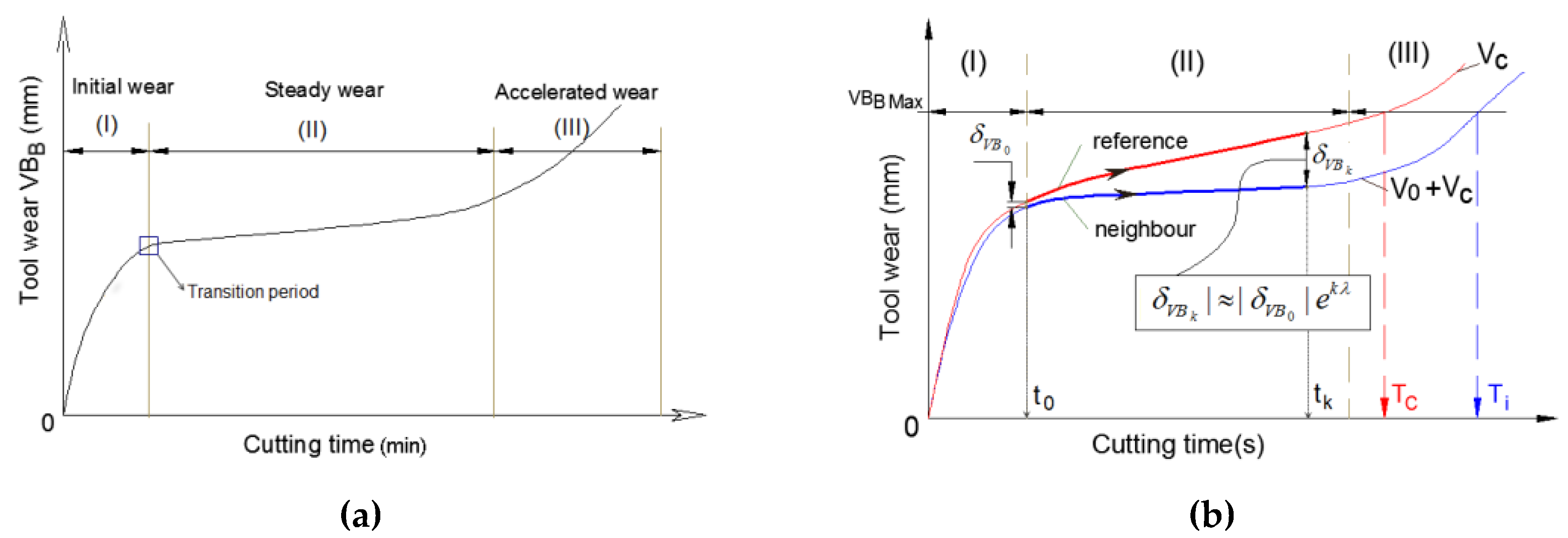
As mentioned earlier, high tool wear rate, short tool life, and poor surface quality are some major issues in machining Ti-MMCs. In addition, the very low thermal conductivity of Ti-MMCs results in very high local temperatures in a small area around the cutting edge, causing a high tool wear rate. This is escalated by tough and abrasive TiC particles dispersed in Ti-MMC, resulting in scratching and grooving of the cutting tools. All of these factors result in a non-linear tool wear rate with three distinctive periods: initial, steady, and accelerated wear (Figure 6a):
As shown in Figure 6b, a slight change in the initial period can significantly change the entire process. This is the foundation of the methodology of this experimental research. Our results show that the initial cutting speed is one of the most critical factors affecting the wear rate and surface roughness over time. This would align with the previous studies [21,35] and a related patent [23], proposing that a protection layer during initial machining is shaped and protects the tool from severe damage and adhesion. In other words, forming a brace shield or a protection layer in the first second of machining is the answer to why tool wear and surface roughness are low with two different cutting speed strategies.
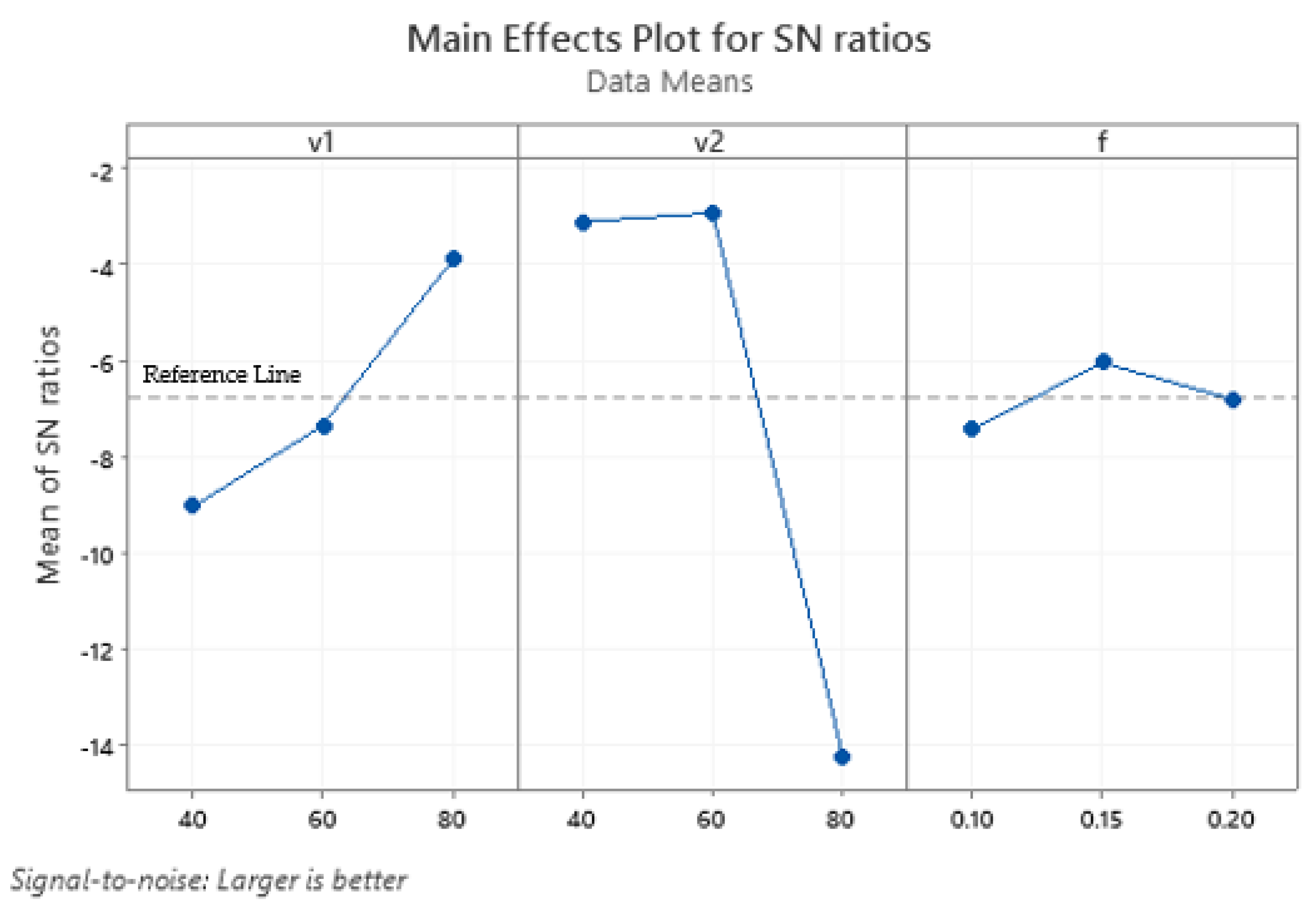
In Figure 7, the mean S/N ratios of the corresponding machining parameter levels for the closeness coefficient ( s i ) is presented. In the main effect plots, when the line is parallel to the x-axis (horizontal), there is not any main effect and the effects of each factor are the same. However, when the line is not horizontal, the effects of each input factor are different and the sharper the slope, the higher magnitude of the main effect. Based on the Taguchi approach, each level of the machining parameters related to the maximum means of the S/N ratios is taken as the optimum setting of the input parameters. As seen in Figure 7, the values of the optimum cutting parameters are identified as the levels (V1− V2 − f) and their respective values are V1 = 80 m/min, V2 = 60 m/min, and f = 0.15 mm/rev. As shown in this plot, with increasing initial speed V1 from 40 to 80 m/min, S/N increases. However, increasing the secondary speed (V2) from 40 to 60 m/min increases S/N and from 60 to 80 m/min decreases S/N. Similarly, with an increasing feed rate from 0.1 to 0.15 mm/rev, S/N increases, and from 0.15 to 0.20 mm/rev, S/N decreases. These results align with other studies [26,29], showing that feed rate affects tool wear less than surface finish. Moreover, a high feed rate can decrease tool wear because of the better heat transfer from the cutting zone to the workpiece.

Probability Plots

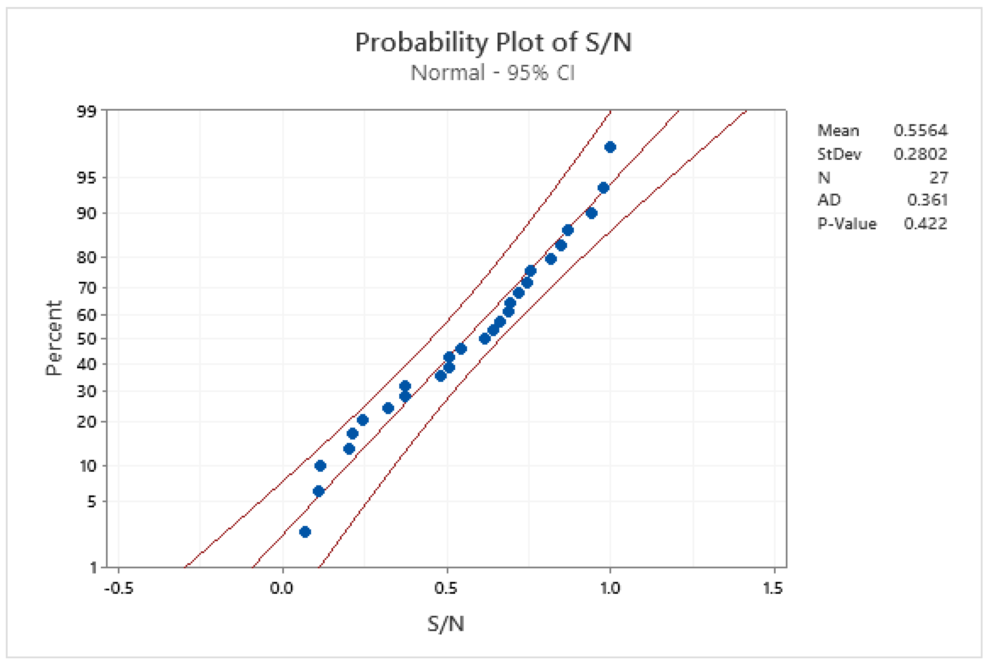
The probability plot shows the distribution of experimental data, as previously presented in Table 4. The Anderson Darling Test (ADT) is a standard statistical tool to validate the normality of assumptions. It shows and detects the outlier from normality [36,37]. The probability plot in Figure 8 confirms that the experimental data for all responses fall near the fitted line and the ADT static values are relatively low (0.361). Furthermore, the p-value (0.422) of the test is also greater than 0.05, meaning that deviation from the null hypothesis is not notable, and the null hypothesis is not rejected. Therefore, it is assumed that the experimental data align with normal distribution and confirm that the study is on the right track.
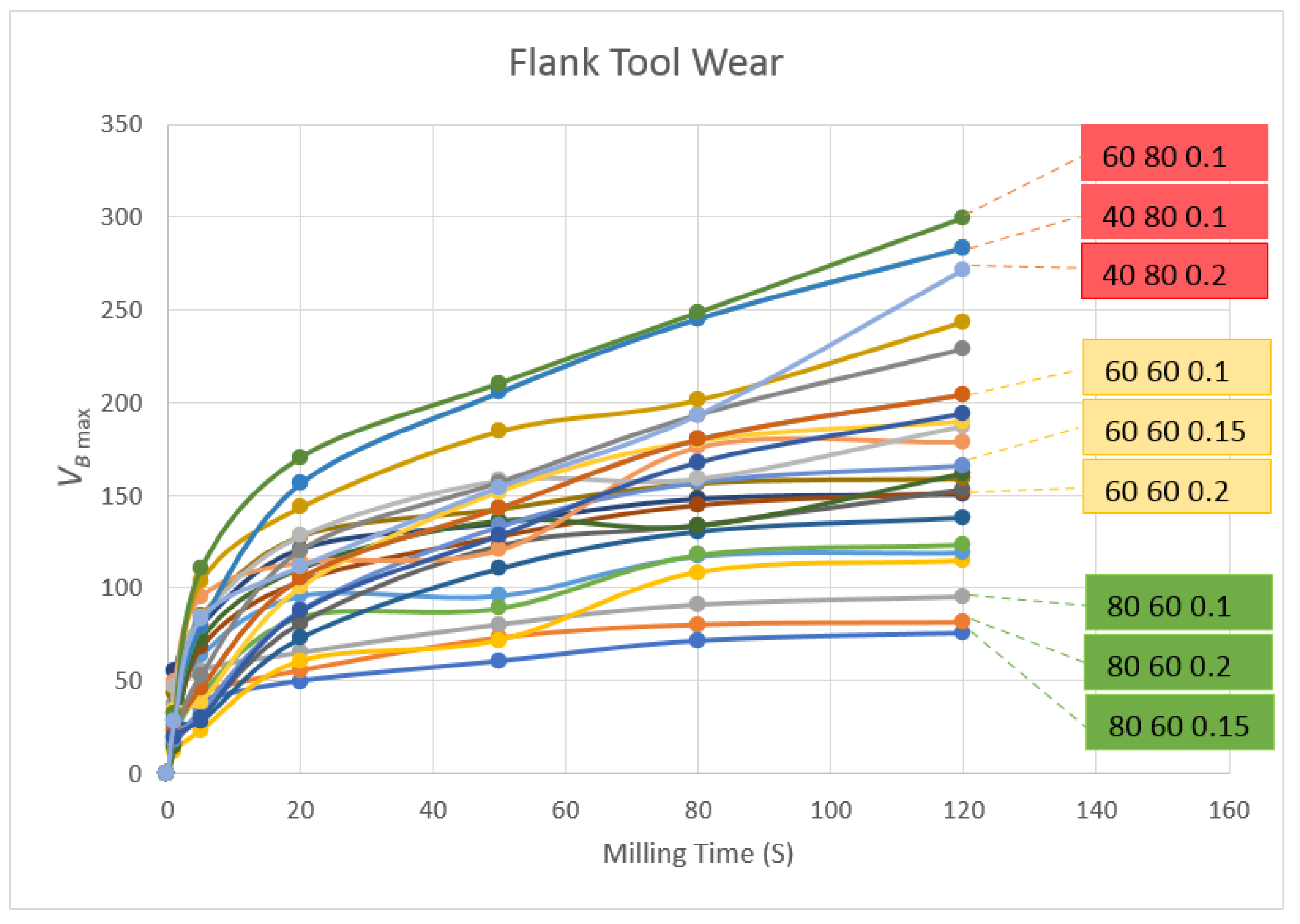
Figure 9 shows the tool wear curves for all 27 cutting conditions. As can be seen, initial cutting speed can significantly affect the tool wear rate. The average of the three lowest tool wear amounts (84.03 µm) is with an initial cutting speed of 80 m/min, secondary cutting speed of 60 m/min, and different feed rates. Traditional machining with 60 mm/min speed and different feed rates has an average tool wear of 172.73 µm. Hence, the strategy of cutting with two different speeds, initial and secondary, can improve tool wear rate by 105.5% compared to traditional machining with a constant cutting speed. Figure 10 also shows the surface roughness results for all 27 cutting conditions. As can be seen, initial cutting speed can also significantly affect surface roughness. The average of the three lowest surface roughness amounts is 1.04 µm, with an initial cutting speed of 80 m/min, secondary cutting speed of 60 m/min, and different feed rates.
Regular machining with 60 m/min speed and different feed rates has an average surface roughness of 2.53 µm. Hence, the strategy of cutting with two different speeds, initial and secondary can improve surface roughness by 143.2% compared to regular machining. Additionally, based on the optimization results, V1 = 80 m/min, V2 = 60 m/min, and f = 0.15 mm/rev are the optimal cutting conditions. It is worth mentioning that the highest tool wear rate is for the secondary cutting speed of 80 m/min and feed rate of 0.1 mm/rev. However, a low initial cutting speed V1 (40 m/min) places two of the experiments among the three highest tool wear rates. Furthermore, the recorded value of surface roughness amount at an initial cutting speed of 40 mm/min, the secondary cutting speed of 80 m/min, and feed rate of 0.15 mm/rev is the highest amount and is similar to tool wear. Low initial cutting speed places two cutting conditions in the highest amounts for surface roughness.

5. Conclusions

This study provides a reliable and structured approach to secure a multi-objective optimization model using the TOPSIS method. The proposed approach led to optimized flank tool wear VB max and surface roughness Ra when milling Ti-MMC. The Taguchi method was used to determine the optimum machining parameters. A L27 full factorial orthogonal array was selected to cover an extensive range of the observed input parameters.
During this work, and within each experimental test, a constant feed rate and different cutting speeds (mainly, initial speed for 1 s (V1) and the secondary (V2) cutting speed for the rest of the machining operation for 120 s0, were used. Flank tool wear VB max and surface roughness R a were the responses. By changing the initial cutting condition for the first second of machining, tool life and surface roughness were improved in all cases of the proposed strategies. It was also found that the values of the optimum cutting parameters are identified as the levels (V1− V2 − f) and their respective values are V1 = 80 m/min, V2 = 60 m/min, and f = 0.15 mm/rev. Moreover, based on the signal-to-noise ratio responses, V2 has the highest impact on the responses and V1 has the second highest impact, meaning it has a higher impact than even the feed rate. Moreover, the strategy of cutting with two different speeds, mainly the initial and the secondary cutting speed, improved wear rate by 105.5% and surface roughness by 143.2% compared to readings made in traditional machining with a constant cutting speed. The observations made in this work align with previous studies on forming a brace shield at the very first moments of machining, acting as a protection layer.
Experimental results confirm that the initial machining conditions significantly affect ultimate tool life. In addition, the significant effects of the initial and secondary cutting speed on the tool wear progress and ultimate tool life were noticed. One of the limitations of the applied methodology is the Taguchi method used to analyze and determine the optimum machining parameters. As mentioned earlier, a L27 full factorial orthogonal array was selected. Therefore, the results are strongly dependent upon the number of the input parameters and do not test all variable combinations. The other limitations are the effects of other machining parameters, such as depth of cut, which has not been studied in this paper. This would be another topic for future work.

Author Contributions

Validation, S.K.; formal analysis, S.K.; investigation, S.K.; writing—original draft preparation, S.K.; writing—review and editing, S.A.N., S.T. and M.B.; supervision and writing—review and editing, S.A.N., S.T. and M.B. All authors have read and agreed to the published version of the manuscript.

Funding

The authors would like to appreciate the financial support received from the Natural Sciences and Engineering Research Council of Canada (NSERC) and NSERC Canadian Network for Research and Innovation in Machining Technology Network (CANRIMT).

Data Availability Statement

Data sharing is not applicable.

Conflicts of Interest

The authors declare no conflict of interest. The funders had no role in the design of the study, in the collection, analyses, or interpretation of data, in the writing of the manuscript, or in the decision to publish the results.

References

  1. Garg, G.K.; Garg, S.; Sangwan, K. Development of an empirical model for optimization of machining parameters to minimize power consumption. In IOP Conference Series: Materials Science and Engineering; IOP Publishing: Bristol, UK, 2018. [Google Scholar]
  2. Kant, G.; Sangwan, K.S. Predictive Modelling and Optimization of Machining Parameters to Minimize Surface Roughness using Artificial Neural Network Coupled with Genetic Algorithm. Procedia CIRP 2015, 31, 453–458. [Google Scholar] [CrossRef] [Green Version]
  3. Kant, G.; Sangwan, K.S. Predictive Modeling for Power Consumption in Machining Using Artificial Intelligence Techniques. Procedia CIRP 2015, 26, 403–407. [Google Scholar] [CrossRef] [Green Version]
  4. Pusavec, F. Sustainable machining of high temperature Nickel alloy–Inconel 718: part 2–chip breakability and optimization. J. Clean. Prod. 2015, 87, 941–952. [Google Scholar] [CrossRef]
  5. Bagaber, S.A.; Yusoff, A.R. Multi-objective optimization of cutting parameters to minimize power consumption in dry turning of stainless steel 316. J. Clean. Prod. 2017, 157, 30–46. [Google Scholar] [CrossRef] [Green Version]
  6. Bilga, P.S.; Singh, S.; Kumar, R. Optimization of energy consumption response parameters for turning operation using Taguchi method. J. Clean. Prod. 2016, 137, 1406–1417. [Google Scholar] [CrossRef]
  7. Kumar, R.; Bilga, P.S.; Singh, S. Multi objective optimization using different methods of assigning weights to energy consumption responses, surface roughness and material removal rate during rough turning operation. J. Clean. Prod. 2017, 164, 45–57. [Google Scholar] [CrossRef]
  8. Hwang, C.-L.; Yoon, K. Methods for multiple attribute decision making. In Multiple Attribute Decision Making; Springer: Berlin/Heidelberg, Germany, 1981; pp. 58–191. [Google Scholar]
  9. Wu, Z.; Abdul-Nour, G. Comparison of multi-criteria group decision-making methods for urban sewer network plan selection. CivilEng 2020, 1, 3. [Google Scholar] [CrossRef]
  10. Rao, S.R.; Jeelani, S.A.K.; Swamulu, V. Multi-objective optimization using TOPSIS in turning of Al 6351 alloy. IOP Conf. Ser. Mater. Sci. Eng. 2021, 1112, 012010. [Google Scholar] [CrossRef]
  11. Mandal, P.; Mondal, S.C. Multi-objective optimization of Cu-MWCNT composite electrode in electro discharge machining using MOPSO-TOPSIS. Measurement 2020, 169, 108347. [Google Scholar] [CrossRef]
  12. Aramesh, M. Machinability of Titanium Metal Matrix Composites (Ti-MMCs); École Polytechnique de Montréal: Montréal, QC, Canada, 2015. [Google Scholar]
  13. Veiga, C.; Davim, J.; Loureiro, A. Review on machinability of titanium alloys: the process perspective. Rev. Adv. Mater. Sci. 2013, 34, 148–164. [Google Scholar]
  14. Zhu, D.; Zhang, X.; Ding, H. Tool wear characteristics in machining of nickel-based superalloys. Int. J. Mach. Tools Manuf. 2013, 64, 60–77. [Google Scholar] [CrossRef]
  15. Konig, W. Applied Research on the Machinability of Titanium and its Alloys. In Proceedings of the AGARD Conference Advanced Fabrication Processes, Florence, Italy, 10 September 1978. [Google Scholar]
  16. Shi, B.; Attia, H.; Tounsi, N. Identification of Material Constitutive Laws for Machining—Part II: Generation of the Constitutive Data and Validation of the Constitutive Law. J. Manuf. Sci. Eng. 2010, 132, 051009. [Google Scholar] [CrossRef]
  17. Jin, L.; Riahi, A.R.; Edrisy, F.A. Investigation on interfacial adhesion of Ti–6Al–4V/nitride coatings. Surf. Coat. Technol. 2014, 260, 155–167. [Google Scholar] [CrossRef]
  18. Bejjani, R. Machinability and Modeling of Cutting Mechanism for Titanium Metal Matrix Composites; École Polytechnique de Montréal: Montréal, QC, Canada, 2012. [Google Scholar]
  19. Liang, L.; Xu, M.; Chen, Y.; Zhang, T.; Tong, W.; Liu, H.; Wang, H.; Li, H. Effect of welding thermal treatment on the microstructure and mechanical properties of nickel-based superalloy fabricated by selective laser melting. Mater. Sci. Eng. A 2021, 819, 141507. [Google Scholar] [CrossRef]
  20. Zhong, M. Mechanical properties of micro laser welding NiTiNb/Ti6Al4V dissimilar alloys lap joints with nickel interlayer. Mater. Lett. 2021, 306, 130896. [Google Scholar] [CrossRef]
  21. Duong, X.T. Chaos Theory Applied to Analyze Tool Wear during Machining of Titanium Metal Matrix Composite (TiMMCs); École Polytechnique de Montréal: Montréal, QC, Canada, 2015. [Google Scholar]
  22. Duong, X.-T.; Balazinski, M.; Mayer, R. Chaotic tool wear during machining of titanium metal matrix composite (TiMMCs). In ASME International Mechanical Engineering Congress and Exposition; American Society of Mechanical Engineers: Montréal, QC, Canada, 2014. [Google Scholar]
  23. Aramesh, M.; Montazeri, S.; Velduis, S. Ultra Soft Cutting Tool Coatings and Coating Method. U.S. Patent 20190314900, 17 October 2019. [Google Scholar]
  24. Abdelali, H.B.; Courbon, C.; Rech, J.; Salem, W.B.; Dogui, A.; Kapsa, P. Identification of a friction model at the tool-chip-workpiece interface in dry machining of a AISI 1045 steel with a TiN coated carbide tool. J. Tribol. 2011, 133, 042201. [Google Scholar] [CrossRef]
  25. Beste, U.; Jacobson, S. A new view of the deterioration and wear of WC/Co cemented carbide rock drill buttons. Wear 2008, 264, 1129–1141. [Google Scholar] [CrossRef]
  26. Kamali Zadeh, S. Initial Tool Wear Mechanisms in Turning of Titanium Metal Matrix Composites; École Polytechnique de Montréal: Montréal, QC, Canada, 2016. [Google Scholar]
  27. Bermingham, M.; Kirsch, J.; Sun, S.; Palanisamy, S.; Dargusch, M. New observations on tool life, cutting forces and chip morphology in cryogenic machining Ti-6Al-4V. Int. J. Mach. Tools Manuf. 2011, 51, 500–511. [Google Scholar] [CrossRef]
  28. Bejjani, R.; Balazinski, M.; Attia, H.; Plamondon, P.; L’Éspérance, G. Chip formation and microstructure evolution in the adiabatic shear band when machining titanium metal matrix composites. Int. J. Mach. Tools Manuf. 2016, 109, 137–146. [Google Scholar] [CrossRef]
  29. Duong, X.; Mayer, J.; Balazinski, M. Initial tool wear behavior during machining of titanium metal matrix composite (TiMMCs). Int. J. Refract. Met. Hard Mater. 2016, 60, 169–176. [Google Scholar] [CrossRef]
  30. Aramesh, M.; Attia, H.M.; Kishawy, H.A.; Balazinski, M. Observation of a unique wear morphology of cBN inserts during machining of titanium metal matrix composites (Ti-MMCs); leading to new insights into their machinability. Int. J. Adv. Manuf. Technol. 2017, 92, 519–530. [Google Scholar] [CrossRef]
  31. Asgari, A. Cutting Conditions Optimisation of Titanium Metal Matrix Composites in Turning and Face Milling; École Polytechnique de Montréal: Montréal, QC, Canada, 2015. [Google Scholar]
  32. Kamalizadeh, S.; Niknam, S.A.; Asgari, A.; Balazinski, M. Tool wear characterization in high-speed milling of titanium metal matrix composites. Int. J. Adv. Manuf. Technol. 2018, 100, 2901–2913. [Google Scholar] [CrossRef]
  33. Sivaiah, P.; Chakradhar, D. Performance improvement of cryogenic turning process during machining of 17-4 PH stainless steel using multi objective optimization techniques. Measurement 2018, 136, 326–336. [Google Scholar] [CrossRef]
  34. Krishnaraj, V.; Samsudeensadham, S.; Sindhumathi, R.; Kuppan, P. A study on High Speed End Milling of Titanium Alloy. Procedia Eng. 2014, 97, 251–257. [Google Scholar] [CrossRef] [Green Version]
  35. Montazeri, S.; Aramesh, M.; Rawal, S.; Veldhuis, S.C. Characterization and machining performance of a chipping resistant ultra-soft coating used for the machining of Inconel 718. Wear 2021, 474, 203759. [Google Scholar] [CrossRef]
  36. Stephens, M.A. EDF statistics for goodness of fit and some comparisons. J. Am. Stat. Assoc. 1974, 69, 730–737. [Google Scholar] [CrossRef]
  37. Qazi, M.I.; Akhtar, R.; Abas, M.; Khalid, Q.S.; Babar, A.R.; Pruncu, C.I. An Integrated Approach of GRA Coupled with Principal Component Analysis for Multi-Optimization of Shielded Metal Arc Welding (SMAW) Process. Materials 2020, 13, 3457. [Google Scholar] [CrossRef]
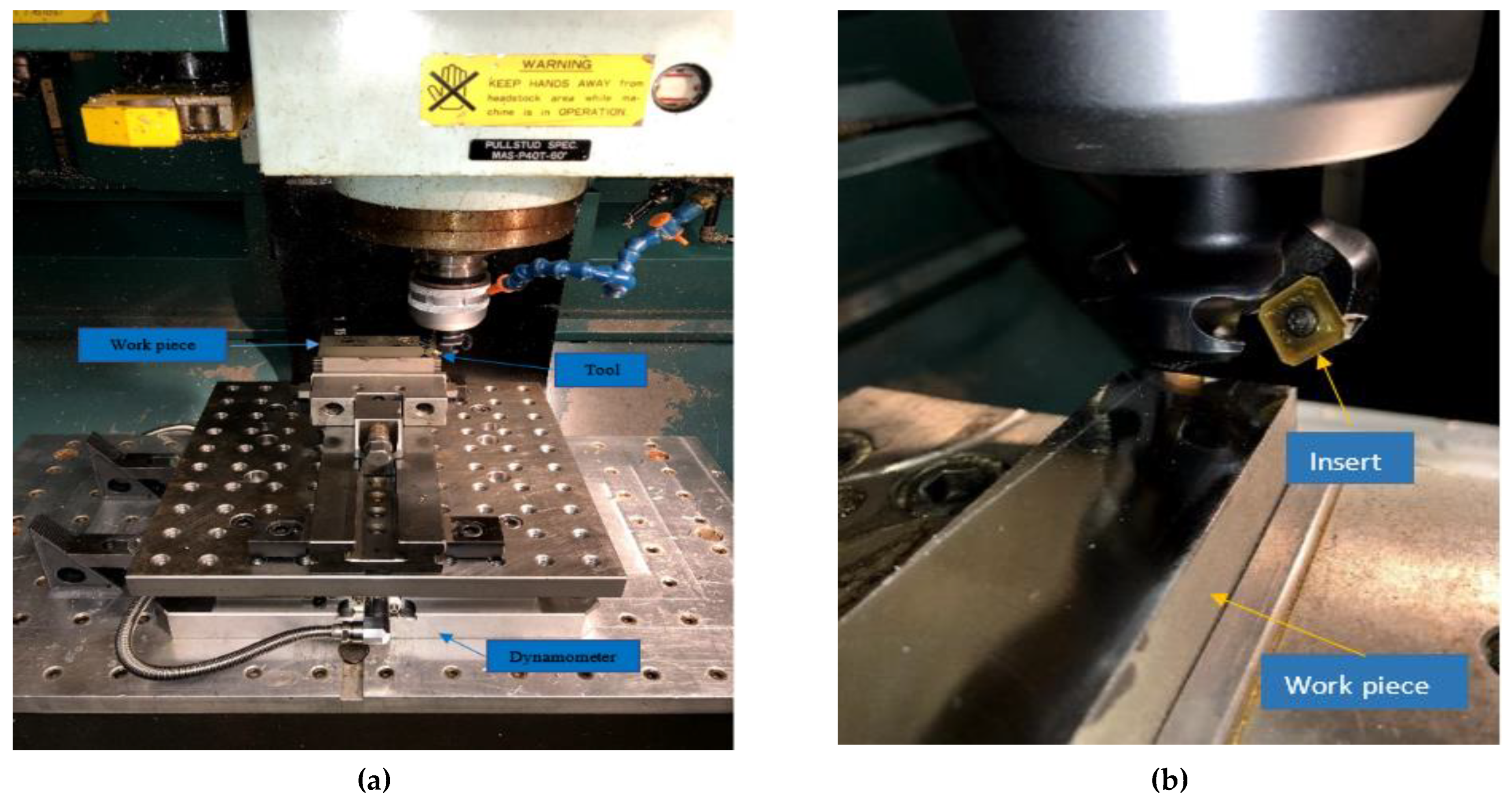
Figure 1. (a) Milling experimental setup and (b) the insert.
Metals 12 01796 g001
Figure 2. (a) Optical microscope and (b) Profilometer Mitutoyo SV-C4000.
Metals 12 01796 g002
Figure 3. A typical tool wear, VB max, and different wear zones [26].
Metals 12 01796 g003
Figure 4. Mean roughness value Ra.
Metals 12 01796 g004
Figure 5. (a) Tool wear after different moments of machining and (b) corresponding captured cutting forces.
Metals 12 01796 g005
Figure 6. (a) Three distinctive tool wear periods; (b) chaos theory: a small change in the initial period can result in a big change in the entire process [21].
Metals 12 01796 g006
Figure 7. Main effect plot for signal-to-noise ratio (S/N) for closeness coefficients.
Metals 12 01796 g007
Figure 8. Probability plot of S/N, data points (blue dots) are relatively close to fitted normal distribution lines.
Metals 12 01796 g008
Figure 9. Tool wear curves for different cutting conditions.
Metals 12 01796 g009
Figure 10. The recorded values of surface roughness under different cutting conditions.
Metals 12 01796 g010
Table 1. Elemental composition of Ti-MMC [32].
Chemical Analysis of TiMMCAluminum
(Al)
Vanadium
(V)
Carbon
(C)
Oxygen
(O)
Iron
(Fe)
Nitrogen
(N)
Hydrogen
(H)
Titanium
(Ti)
Mass %5.553.840.970.260.0040.21<0.003Remainder (89.163)
Table 2. CoroMill 245-12T3 carbide tool.
CoroMill 245 PVD TiAlN + TiNInsert Specifications
Metals 12 01796 i001Inscribed circle diameter (IC)13.4 mm
Cutting edge effective length (LE)10 mm
Insert rake angle (GAN)15 deg
Corner radius (RE)1.5 mm
Coating (COATING)PVD TiAlN + TiN
Substrate (SUBSTRATE)Coated carbide/Cermet (HC)
Table 3. Considered input cutting parameters.
Levels/ParametersInitial Cutting Speed V1 (m/min)Secondary Cutting Speed V2 (m/min)Feed Rate
f (mm/rev)
I40400.1
II60600.15
III80800.2
Table 4. Input cutting parameters and their responses.
Experimental RunExperimental ParametersResponses
V1 (m/min)V2 (m/min)f (mm/rev) R a VB max (µm)
140400.11.907220.2
240400.151.999232.2
340400.21.776194.2
440600.11.684179
540600.151.902138
640600.21.769159
740800.13.685296.3
840800.154.185228.6
940800.23.983283.6
1060400.11.284114.5
1160400.151.257123.5
1260400.21.517153
1360600.12.514204.5
1460600.152.884162
1560600.22.194151.7
1660800.13.687299.3
1760800.153.318271.2
1860800.23.447243.5
1980400.11.683166.3
2080400.151.483150.4
2180400.21.565119.2
2280600.11.02395.4
2380600.151.02875.4
2480600.21.08381.3
2580800.13.43187.5
2680800.153.381189.4
2780800.23.574201.3
Table 5. Normalized weighted values of the responses.
Experimental RunNormalized ValueWeighted Normalized Value
R a   VB max (µm) R a VB max
1143.9418220.5420.07190.1102
2150.8861232.5610.07540.1162
3134.0538194.5020.06700.0972
4127.1096179.2780.06350.0896
5143.5644138.2140.07170.0691
6133.5255159.2470.06670.0796
7278.1466296.760.13900.1483
8315.887228.9550.15790.1144
9300.6399284.040.15030.1420
1096.9173114.6780.04840.0573
1194.8793123.6920.04740.0618
2114.5043153.2380.05720.0766
13189.7587204.8180.09480.1024
14217.6865162.2520.10880.0811
15165.6048151.9360.08280.0759
16278.2976299.7650.13910.1498
17250.4452271.6210.12520.1358
18260.1822243.8780.13000.1219
19127.0341166.5580.06350.0832
20111.938150.6340.05590.0753
21118.1274119.3850.05900.0596
2277.216875.5170.03860.0377
2377.594279.7240.03870.0398
2481.745781.4260.04080.0407
25258.899187.7910.12940.0938
26255.2005189.6940.12760.0948
27269.7683201.6130.13480.1008
Table 6. Separation measures, closeness coefficient, and signal-to-noise ratios.
Experimental RunSeparation Measures Closeness CoefficientSignal-to-Noise Ratio
d i b d i w s i S/N
10.07960.09470.5431−5.302
20.08650.08910.5072−5.8952
30.06580.10510.6149−4.22267
40.05740.11200.6610−3.5956
50.04550.11810.7216−2.83334
60.05030.11510.6957−3.15058
70.14920.01890.1126−18.9671
80.14170.03550.2005−13.9564
90.15260.01100.0677−23.3833
100.02180.14340.8677−1.23165
110.02550.14130.8467−1.44461
20.04300.12450.7433−2.57565
130.08560.07900.4800−6.37498
140.08240.08450.5062−5.91241
150.05830.10540.6438−3.82474
160.15040.01870.1110−19.0889
170.13060.03560.2145−13.3704
180.12420.03950.2416−12.3371
190.05170.11560.6906−3.21494
200.04120.12630.7537−2.45495
210.02990.13380.8172−1.75247
220.00990.15710.9404−0.53337
230.00010.16360.9988−0.01039
240.00360.16010.9775−0.19727
250.10670.06290.3709−8.6133
260.10560.06290.3733−8.55673
270.11500.05430.3209−9.87205
Table 7. Responses for signal-to-noise ratios (larger is better).
LevelV1V2f
1−9.034−3.122−7.436
2−7.351−2.937−6.048
3−3.912−14.238−6.813
Delta5.12211.3011.387
Rank213
Publisher’s Note: MDPI stays neutral with regard to jurisdictional claims in published maps and institutional affiliations.