Isogeometric Analysis-Based Solidification Simulation and an Improved Way to Apply Supercooling on Droplet Boundary

Abstract

The classic finite difference method (FDM) has been successfully adopted in the simulation of dendritic solidification, which is based on phase-field theory. Nevertheless, special strategies of boundary integral and projection are required for applying a supercooling rate to a droplet surface. In the present study, isogeometric analysis (IGA) is employed to discretize the phase-field equation due to the two advantages of Non-Uniform Rational B-Splines (NURBS) basis functions, namely an arbitrary order of derivatives and exact description of complex geometry. In addition, an improved, easy way to apply the supercooling rate on a melt droplet surface is proposed to avoid the integral and projection of the cellular boundary required in FDM. Firstly, dendrite growth in a square computational domain is simulated to verify the performance of IGA. Then, the influences of latent heat, anisotropic mode and initial angle on the dendrite shapes are studied by the presented IGA, FDM and finite element method (FEM). Finally, dendritic solidification in a droplet under different cooling rates along irregular boundaries is performed by the proposed IGA.

1. Introduction

Dendrite growth is an essential phenomenon of phase transition in material science [1,2]. In the casting of metals and alloys, molten metals first generate tiny embryos in the liquid phase and then gradually grow into a stable crystal nucleus. Under the effect of supercooling, they grow up continuously into different structures and finally complete the process of solidification [3]. The final morphology of crystal growth has a direct impact on the properties of materials, such as mechanical strength, corrosives, electrical conductivity and ductility [4]. Numerical technology could provide the ability to gain insight into the interior quality analysis of casting products. It assists engineers in observing the evolution of microstructures in the metal solidification process under different conditions and parameters and thus improves product quality. Furthermore, it helps to control the dendrite growth to obtain the required material properties. Based on the finite difference method (FDM), a special way to calculate the boundary cooling term for a droplet surface was proposed by Miura et al. [5] to avoid overestimated surface length, as shown in Figure 1. Inspired by their work to study the effects of supercooling rates on solidification in droplets, we conducted similar research via IGA with an improved reaction equation for temperature dynamics by introducing an extra term for supercooling on the droplet boundary. Thus, additional calculations of projection lengths of cellular boundary edges and integrals over surfaces are avoided.

Up to now, the phase field method has been commonly applied in material science [6,7], crystal nucleation and growth [8,9,10], fracture mechanics [11,12], heat transfer [13,14,15,16,17], fluid–structure interaction [18,19] and biomechanics [20,21,22,23,24,25,26,27,28]. Taking the example in solidification of pure metal, there are two phases in the whole studied domain, namely liquid and solid phases whose order parameters $\varphi$ take values of 0 and 1, respectively. The value of the interface phase between these two phases varies in the interval $\left(0,1\right)$. The dynamic of the interface is driven by the free energy difference between the two phases [29]. As shown in Figure 2, the non-conservative phase field $\varphi$ has two local stable phases with $\varphi =0$ and $\varphi =1$, respectively. However, the interface phase $0<\varphi <1$ is meta-stable and has a tendency to jump from high energy to low energy. As a consequence, the interface moves from one phase to the other, and phase transition is achieved automatically without tracking the interface front. Nevertheless, the phase filed equation involves the computation of high-order derivatives with respect to order parameter. Usually, the high-order finite element method (FEM) and finite difference method [30,31,32,33] are used to solve the high-order partial differential equation. The former brings about more computational efforts due to extra freedoms. The latter is particularly limited to the regular domain. In order to solve the above problems, IGA is adopted to simulate the dendrite growth in this study [34].

Isogeometric analysis was first proposed by Hughes [35] in 2005 for the seamless integration of computer-aided design (CAD) and computer-aided engineering (CAE) and has been widely used in crack [36,37,38], vibration [39,40,41], heat transfer and fluid–structure interaction [18,42,43,44], and optimization of practical engineering problems [45,46,47,48]. It can not only accurately describe the complex geometric shape of the object but also has an arbitrary-order partial derivative in theory due to the use of NURBS basis functions and has been proven very successful for phase-field equations [43,44,49,50,51]. In the work of reference [50], the application of IGA in phase-field is reviewed and a general example of solidification is given. In the present work, the computational framework of IGA is proposed to analyze solidification and study the effects of several parameters on dendrite growth. In addition, a special strategy for boundary supercooling is presented, and corresponding findings with different cooling rates are compared with experimental observations.

This paper is organized as follows: Section 2 describes the phase-field based mathematical model for dendrite growth and the reaction-diffusion equation for temperature dynamics. The NURBS basis functions of IGA, their derivatives and the integration scheme are introduced in Section 3. Section 4 presents the IGA-based computational framework of the phase-field and reaction-diffusion equation of temperature dynamics for solidification simulation. Then, the process of the generalized-$\alpha$ method for solving the equations is illustrated. In Section 5, a square domain is used to test the performance of the presented method for dendrite growth, and the effects of several parameters on crystal growth are discussed. The computational efficiency of the proposed method is then compared with FDM and FEM. Moreover, an extra term is added to the dynamic equation of temperature to study the effects of supercooling rate on solidification. Three values of cooling rates are tested, and the results are validated with the work of references [5,52]. Finally, we conclude with a summary in Section 6.

2. Mathematical Model

In this study, the phase-field equation is applied to describe the process of dendrite growth, and a reaction–diffusion equation is adopted for the dynamics of temperature. The variable $\varphi (x,y,t)$ is taken as the order parameter in the phase-field model, representing the solid phase with $\varphi (x,y,t)=1$ and liquid phase with $\varphi (x,y,t)=0$ at position $(x,y)$ at time t. There is automatically a smoothing interface $0<\varphi (x,y,t)<1$ between the two phases. For the purpose of convenience, $\varphi (x,y,t)$ is simply written as $\varphi$. The free energy functional for driving the phase transition of the system is defined as

$$F(\varphi ,m)={\int }_{\mathsf{\Omega }}\left[{\displaystyle \frac{1}{2}}{\epsilon }^2{\left|\nabla \varphi \right|}^2+\psi (\varphi ,T)\right]\mathrm{d}\mathsf{\Omega }$$

(1)

where $\epsilon$ is a constant related to the interface width. The first term in the integral of Equation (1) is the interface free energy and the second term $\psi (\varphi ,T)$ is the chemical free energy, a double-well potential with two local minima at $\varphi =0$ and $\varphi =1$. The specific expression of $\psi (\varphi ,T)$ is chosen as

$$\psi (\varphi ,T)={\displaystyle \frac{1}{4}}{\varphi }^4-\left({\displaystyle \frac{1}{2}}-{\displaystyle \frac{1}{3}}m\right){\varphi }^3+\left({\displaystyle \frac{1}{4}}-{\displaystyle \frac{1}{2}}m\right){\varphi }^2$$

(2)

where m is a function of supercooling, acting as a thermodynamic driving force, and is defined as

$$m\left(T\right)={\displaystyle \frac{\alpha }{\pi }}arctan\left(\gamma (T_{eq}-T)\right)$$

(3)

where $T_{eq}$ is the melting temperature, taking the value of 1 in this paper. Temperature field T is normalized to the interval $[0,1]$. $\alpha$ and $\gamma$ are constants. As shown in Figure 2, the $\psi (\varphi ,T)$ has two local minima at $\varphi =0$ and $\varphi =1$. The dynamic system tends to be stable, which leads to a decrease in energy. The metastable state of phase at the interface turns out to be the local stable phase. When the temperature T at interfacial phase $0<\varphi <1$ is less than the balance temperature $T_{eq}$, namely $m>0$, the interface phase will be driven to be solid phase $\varphi =1$ since the interface phase changes from a high energy state to a low energy state. If the temperature T is greater than $T_{eq}$, the opposite situation happens, and the liquid phase grows.

In practice, the morphology of dendrite growth is anisotropic. In order to capture the anisotropic characteristic of crystal, the function of interfacial width $\epsilon$ is introduced as follows

$$\epsilon \left(\theta \right)=\overline{\epsilon }\left[1+\delta cos\left(j\left(\theta -{\theta }_0\right)\right)\right]$$

(4)

where $\overline{\epsilon }$ is the phase width and determines the thickness of the interface layer; $\delta$ is the strength of interface width; j is the mode number of anisotropy; $\theta$ is the angle between the outward normal direction of the interface and the x axis; ${\theta }_0$ is the initial angle that represents the orientation of the anisotropic axis.

The free energy of the system Equation (1) is required to decrease monotonically with time. Considering the concept of gradient dynamics [53], the non-conserved phase-field equation for solidification is defined as

$$\tau {\displaystyle \frac{\partial \varphi }{\partial t}}=-{\displaystyle \frac{\delta F}{\delta \varphi }}$$

(5)

Substituting Equations (2)–(4) into Equation (1), then, Equation (5) can be derived as

$$\tau {\displaystyle \frac{\partial \varphi }{\partial t}}=-{\displaystyle \frac{\partial }{\partial x}}\left(\epsilon {\epsilon }^{{}^{\prime }}{\displaystyle \frac{\partial \varphi }{\partial y}}\right)+{\displaystyle \frac{\partial }{\partial y}}\left(\epsilon {\epsilon }^{{}^{\prime }}{\displaystyle \frac{\partial \varphi }{\partial x}}\right)+\nabla ·{\epsilon }^2\nabla \varphi -\mu (\varphi ,T)$$

(6)

where ${\epsilon }^{{}^{\prime }}=d\epsilon /d\theta$; $\mu (\varphi ,T)$ is the derivative of chemical free energy with respect to $\varphi$ and given by

$$\begin{array}{c}\hfill \mu (\varphi ,T)={\varphi }^3-(1.5-m){\varphi }^2+(0.5-m)\varphi =-\varphi (1-\varphi )(\varphi -0.5+m)\end{array}$$

(7)

According to references [54,55], the dynamics of the temperature field are described by a reaction–diffusion equation can be rewritten as follows

$${\displaystyle \frac{\partial T}{\partial t}}=\nabla ·\nabla T+K{\displaystyle \frac{\partial \varphi }{\partial t}}$$

(8)

where K is the dimensionless latent heat. The second term on the right side of Equation (8) accounts for the release of latent heat at the interface. Equations (6) and (8) are in dimensionless units. The modified equation of temperature dynamic for applying supercooling on a droplet surface is presented in Section 5.2.

3. NURBS Shape Functions in Isogeometric Analysis

As an extension of FEM, IGA aims to accomplish the seamless integration of CAD and CAE [35]. In the implementation of IGA, the NURBS basis functions are used instead of the classical Lagrangian shape functions in FEM. The unknowns to be solved are the physical variables at control points, no longer at nodes of elements. In this section, the NURBS bases and numerical integration are introduced.

3.1. B-Splines

B-spline is a basis spline function that has local support with a given degree, knot partition and control points. The knot vector in a B-spline is defined as $U=\{u_1,u_2,\cdots ,u_{n+p+1}\}$ in a non-descending order. $u_i$ is the ith knot, n is the number of basis functions and p is the polynomial order [35]. The knot interval could be uniform, non-uniform, or even 0 where more than one knot repeats at the same partition position i. According to the Cox-de Boor recursion formula [56], the B-Spline basis functions are given for a polynomial order $\mathit{p}=0$

$$N_{i,0}\left(u\right)=\left\{\begin{array}{cc}1\hfill & u_i⩽u<u_{i+1}\hfill \\ 0\hfill & \mathrm{otherwise}\hfill \end{array}\right.$$

(9)

and for a polynomial order $\mathit{p}\ge 1$

$$\begin{array}{c}\hfill N_{i,p}\left(u\right)={\displaystyle \frac{u-u_i}{u_{i+p}-u_i}}{N}_{i,p-1}\left(u\right)+{\displaystyle \frac{u_{i+p+1}-u}{u_{i+p+1}-u_{i+1}}}{N}_{i+1,p-1}\left(u\right)\end{array}$$

(10)

where $N_{i,p}\left(u\right)$ is ith B-spline basis function of order p. The ratio in the form of $0/0$ is defined as zero in the process of calculating the bases. Some important properties of B-spline basis functions are listed as

•

$N_{i,p}\left(u\right)$ is a polynomial over $u_i$;

•

$N_{i,p}\left(u\right)$ is non-negativity $N_{i,p}\left(u\right)\ge 0$;

•

Each p order function $N_{i,p}\left(u\right)$ has $p-1$ continuous derivatives across the element boundary when the knot multiplicity is one for all inner knots. The first derivative of a B-spline basis function can be easily calculated from the Cox-de Boor recursion formula

$$\begin{array}{c}\hfill {\displaystyle \frac{d}{du}}{N}_{i,p}\left(u\right)={\displaystyle \frac{p}{u_{i+p}-u_i}}{N}_{i,p-1}\left(u\right)-{\displaystyle \frac{p}{u_{i+p+1}-u_{i+1}}}{N}_{i+1,p-1}\left(u\right)\end{array}$$

(11)

•

If k is the multiplicity of the ith knot, $N_{i,p}\left(u\right)$ is ${\mathcal{C}}^{p-k}$ continuous.

Then, a B-spline curve can be a linear combination of B-spline basis functions and is described as follows

$$C\left(u\right)=\sum _{i=1}^n{N}_{i,p}\left(u\right)P_i$$

(12)

where $P_i$ is the ith control point ($i=1,2,\cdots ,n$).

With two known knot vectors $U=\{u_1,u_2,\cdots ,u_{n+p+1}\}$ and $V=\{v_1,v_2,\cdots ,v_{l+q+1}\}$, and $(n+1)\times (l+1)$ control points, a B-spline surface is given by

$$S(u,v)=\sum _{i=1}^n\sum _{j=1}^l{N}_{i,p}\left(u\right)N_{j,q}\left(v\right)P_{ij}$$

(13)

where $P_{ij}$ is a control point.

3.2. NURBS Shape Function

Although B-spline possesses good properties, it can not represent circles, spheres, ellipsoids and paraboloids exactly. In order to overcome this disadvantage, a NURBS curve of order $\mathit{p}$ is presented as a linear combination of B-spline bases by introducing weighting function

$$C\left(u\right)=\sum _{i=1}^n{R}_i\left(u\right)P_i$$

(14)

where $R_i\left(u\right)$, the NURBS basis function, is written as

$$R_i\left(u\right)={\displaystyle \frac{N_{i,p}\left(u\right)w_i}{{\sum }_{i=1}^n{N}_{i,p}\left(u\right)w_i}}$$

(15)

$w_i$ is the weighting function in 1D.

Similarly, the NURBS surface can be expressed as

$$S(u,v)=\sum _{i=1}^n\sum _{j=1}^l{R}_{i,j}(u,v)P_{ij}$$

(16)

The bivariate basis function $R_{i,j}(u,v)$ is written as

$$R_{i,j}(u,v)={\displaystyle \frac{N_{i,p}\left(u\right)N_{j,q}\left(v\right)w_{ij}}{{\sum }_{i=1}^n{\sum }_{j=1}^l{N}_{i,p}\left(u\right)N_{j,q}\left(v\right)w_{ij}}}$$

(17)

where $w_{ij}$ is the weighting function in 2D. In what follows, NURBS shape function R is symbolically replaced with N.

3.3. Numerical Integration in IGA

For the purpose of simplicity, only numerical integration over a 2D computational domain is presented herein. The integration scheme for 3D is not addressed in this work and can be easily obtained by just adding variables in the third dimension. As shown in Figure 3, there are three domains, namely the physical domain ${\mathsf{\Omega }}^e$, parametric domain ${\widehat{\mathsf{\Omega }}}^e$ and parent domain ${\overline{\mathsf{\Omega }}}^e$. The numerical integration over the whole physical domain ($\mathsf{\Omega }=\bigsqcup {\mathsf{\Omega }}^e$, ${\mathsf{\Omega }}^e$ is the elemental domain) can be calculated through two main mapping steps, which are expressed as

$$\begin{array}{cc}\hfill & {\int }_{\mathsf{\Omega }}f(x,y)\mathrm{d}\mathsf{\Omega }\hfill \\ \hfill & =\sum _{e=1}^{n_e}{\int }_{{\mathsf{\Omega }}^e}f(x,y)\mathrm{d}{\mathsf{\Omega }}^e\hfill \\ \hfill & =\sum _{e=1}^{n_e}{\int }_{{\widehat{\mathsf{\Omega }}}^e}f\left(x\left(\widehat{\xi }\right),y\left(\widehat{\eta }\right)\right)|\widehat{J}|\mathrm{d}{\widehat{\mathsf{\Omega }}}^e\hfill \\ \hfill & =\sum _{e=1}^{n_e}{\int }_{{\overline{\mathsf{\Omega }}}^e}f\left(x\left(\overline{\xi }\right),y\left(\overline{\eta }\right)\right)|\widehat{J}\left|\right|\overline{J}|\mathrm{d}{\overline{\mathsf{\Omega }}}^e\hfill \end{array}$$

(18)

where $f(·,·)$ is the function to be integrated, and $n_e$ is the number of elements (different from those in FEM, elements in IGA are related with a knot partition). $|\widehat{J}|$ and $|\overline{J}|$ are determinants of the two Jacobian matrices for geometry mapping. The first Jacobian $\widehat{J}$ between the physical elemental domain and the parametric domain is given as

$$\widehat{J}=\left[\begin{array}{cc}{x}_{,\widehat{\xi }}& x_{,\widehat{\eta }}\\ y_{,\widehat{\xi }}& y_{,\widehat{\eta }}\end{array}\right]$$

(19)

and the other Jacobian between the parametric and parent domains $\overline{J}=0.25({\widehat{\xi }}_{i+1}-{\widehat{\xi }}_i)({\widehat{\eta }}_{i+1}-{\widehat{\eta }}_i)$. Then, a numerical integration scheme in FEM can be applied in the last term in Equation (18).

4. Computational Method

4.1. Spatial Discretization

Let us define the trial and weighting function spaces $\mathcal{V}\subset {\mathcal{H}}^2\left(\mathsf{\Omega }\right)$. Here, ${\mathcal{H}}^2\left(\mathsf{\Omega }\right)$ is the Sobolev space of integrable functions in the domain $\mathsf{\Omega }$. The finite-dimensional space for discretization is expressed as ${\mathcal{V}}^h=\mathrm{span}{\left\{N_i\right\}}_{i=1,2,\cdots ,n}$, where n is the dimension of ${\mathcal{V}}^h\subset \mathcal{V}\subset {\mathcal{H}}^2\left(\mathsf{\Omega }\right)$, and the $N_i$’s are linearly independent NURBS basis functions [24,25,28]. Taking the weighting function $\omega$ as a trial function, the Galerkin weak form of Equations (6) and (8) can be expressed as

$$\begin{array}{cc}& {\int }_{\mathsf{\Omega }}{\omega }^h·\tau {\displaystyle \frac{\partial {\varphi }^h}{\partial t}}d\mathsf{\Omega }={\int }_{\mathsf{\Omega }}{\omega }^h·[-{\displaystyle \frac{\partial }{\partial x}}\left(\epsilon {\epsilon }^{{}^{\prime }}{\displaystyle \frac{\partial {\varphi }^h}{\partial y}}\right){\displaystyle \frac{\partial }{\partial y}}\left(\epsilon {\epsilon }^{{}^{\prime }}{\displaystyle \frac{\partial {\varphi }^h}{\partial x}}\right)+\nabla ·{\epsilon }^2\nabla {\varphi }^h-\mu ({\varphi }^h,T^h)]d\mathsf{\Omega }\hfill \end{array}$$

(20)

$$\begin{array}{cc}& {\int }_{\mathsf{\Omega }}{\omega }^h·{\displaystyle \frac{\partial T^h}{\partial t}}d\mathsf{\Omega }={\int }_{\mathsf{\Omega }}{\omega }^h·\nabla ·\nabla T^{h}d\mathsf{\Omega }+{\int }_{\mathsf{\Omega }}{\omega }^h·K{\displaystyle \frac{\partial {\varphi }^h}{\partial t}}d\mathsf{\Omega }\hfill \end{array}$$

(21)

After applying the integral by parts and divergence theorem (see Appendix A for details), the Galerkin weak form of Equations (20) and (21) can be written as

$$\begin{array}{c}\hfill {\int }_{\mathsf{\Omega }}\left[-\left({\displaystyle \frac{\partial {\omega }^h}{\partial x}},{\displaystyle \frac{\partial {\omega }^h}{\partial y}}\right)·\left(\epsilon \epsilon {\displaystyle \frac{\partial {\varphi }^h}{\partial x}},\epsilon \epsilon {\displaystyle \frac{\partial {\varphi }^h}{\partial y}}\right)\right]\mathrm{d}\mathsf{\Omega }\\ \hfill -{\int }_{\mathsf{\Omega }}\left[\left({\displaystyle \frac{\partial {\omega }^h}{\partial y}}\right),{\displaystyle \frac{\partial {\omega }^h}{\partial x}}\right]·\left(\epsilon {\epsilon }^{{}^{\prime }}\right){\displaystyle \frac{\partial {\varphi }^h}{\partial x}},-\epsilon {\epsilon }^{{}^{\prime }}{\displaystyle \frac{\partial {\varphi }^h}{\partial y}}\end{array}$$

(22)

$$\begin{array}{cc}& {\int }_{\mathsf{\Omega }}{\omega }^h·{\displaystyle \frac{\partial T^h}{\partial t}}d\mathsf{\Omega }+{\int }_{\mathsf{\Omega }}\nabla {\omega }^h·\nabla T^{h}d\mathsf{\Omega }-{\int }_{\mathsf{\Omega }}{\omega }^h·K{\displaystyle \frac{\partial {\varphi }^h}{\partial t}}d\mathsf{\Omega }=0\hfill \end{array}$$

(23)

The discrete solution $\varphi$ and T are defined as

$$\begin{array}{c}\hfill \varphi {(x,y,t)}^h=\sum _{i=1}^n{\varphi }_i\left(t\right)N_i(x,y),\end{array}$$

(24)

$$\begin{array}{c}\hfill T{(x,y,t)}^h=\sum _{i=1}^n{T}_i\left(t\right)N_i(x,y),\end{array}$$

(25)

respectively. The ${\varphi }_i$ and $T_i$ are the control variables. The weighting function ${\omega }^h$ is expressed as

$$\omega {(x,y)}^h=\sum _{i=1}^n{\omega }_i{N}_i(x,y)$$

(26)

where the ${\omega }_i$ is the control variable.

4.2. Time Discretization

The dynamic Equations (22) and (23) are discretized by the generalized-$\alpha$ method [57] and solved by the Newton–Raphson method. Notations ${\overrightarrow{\Phi }}_n$ and ${\overrightarrow{T}}_n$ are used for the global vector of control variables of the unknowns ${\varphi }_n^h$ and $T_n^h$ where the subscript n refers to the time step. We call ${\dot{\overrightarrow{\Phi }}}_n$ and ${\dot{\overrightarrow{T}}}_n$ the time derivatives of the control variable vectors. We further introduce ${\overrightarrow{S}}_n=\{{\overrightarrow{\Phi }}_n,{\overrightarrow{T}}_n\}$. Using this notation, the residual vectors are defined as

$$\begin{array}{cc}& R_A^{\varphi }\left({\overrightarrow{S}}_{n+{\alpha }_f},{\dot{\overrightarrow{S}}}_{n+{\alpha }_m}\right)={\left(N_A,\tau {\dot{\varphi }}_{n+{\alpha }_m}^h\right)}_{\mathsf{\Omega }}+{\left(\nabla N_A,{\epsilon }^2\nabla {\varphi }_{n+{\alpha }_f}^h\right)}_{\mathsf{\Omega }}-{\left(\nabla N_A^{{}^{\prime }},\epsilon {\epsilon }^{{}^{\prime }}\nabla {\varphi }_{n+{\alpha }_f}^h\right)}_{\mathsf{\Omega }}+{\left(N_A,{\mu }_{\varphi }\left({\varphi }_{n+{\alpha }_f}^h,T_{n+{\alpha }_f}^h\right)\right)}_{\mathsf{\Omega }}\hfill \end{array}$$

(27)

$$\begin{array}{cc}& R_A^T\left({\overrightarrow{S}}_{n+{\alpha }_f},{\dot{\overrightarrow{S}}}_{n+{\alpha }_m}\right)={\left(N_A,{\dot{T}}_{n+{\alpha }_m}^h\right)}_{\mathsf{\Omega }}+{\left(\nabla N_A,\nabla T_{n+{\alpha }_f}^h\right)}_{\mathsf{\Omega }}-{\left(N_A,K{\dot{\varphi }}_{n+{\alpha }_m}^h\right)}_{\mathsf{\Omega }}\hfill \end{array}$$

(28)

where $(·,·)$ is the inner product in the domain $\mathsf{\Omega }$. $\nabla N_A=\left(\partial N_A/\partial x,\partial N_A/\partial y\right)$. $\nabla N_A^{{}^{\prime }}=\left(\partial N_A/\partial y,\partial N_A/\partial x\right)$. Variables at the intermediate time level are given as [28,35]

$$\begin{array}{cc}& {\dot{\overrightarrow{S}}}_{n+{\alpha }_m}^h={\dot{\overrightarrow{S}}}_n^h+{\alpha }_m\left({\dot{\overrightarrow{S}}}_{n+1}^h-{\dot{\overrightarrow{S}}}_n^h\right)\hfill \end{array}$$

(29)

$$\begin{array}{cc}& {\overrightarrow{S}}_{n+{\alpha }_f}^h={\overrightarrow{S}}_n^h+{\alpha }_f\left({\overrightarrow{S}}_{n+1}^h-{\overrightarrow{S}}_n^h\right)\hfill \end{array}$$

(30)

$$\begin{array}{cc}& {\overrightarrow{S}}_{n+1}^h={\overrightarrow{S}}_n^h+\mathsf{\Delta }{t}_n{\dot{\overrightarrow{S}}}_n^h+\gamma \mathsf{\Delta }{t}_n\left({\dot{\overrightarrow{S}}}_{n+1}^h-{\dot{\overrightarrow{S}}}_n^h\right)\hfill \end{array}$$

(31)

Then, solve the below linear system using the generalized minimal residual method algorithm

$${\overrightarrow{K}}_{n+1}^i\mathsf{\Delta }{\dot{\overrightarrow{S}}}_{n+1}^i=-{\overrightarrow{R}}_{n+1}^i$$

(32)

where $\mathsf{\Delta }{\dot{\overrightarrow{S}}}_{n+1}^i$ is the increment of time derivatives of the control variable vectors in each iteration. The tangent matrix involved in the ith iteration is given as

$${\overrightarrow{K}}_{n+1}^i=\partial {\overrightarrow{R}}_{n+1}^i\partial /{\dot{\overrightarrow{S}}}_{n+1}^i$$

(33)

Following the instruction in reference [57], we take

$${\alpha }_m=\frac{1}{2}\left(\frac{3-{\rho }_{\infty }}{1+{\rho }_{\infty }}\right);{\alpha }_f=\frac{1}{1+{\rho }_{\infty }};\gamma =\frac{1}{2}+{\alpha }_m-{\alpha }_f.$$

(34)

The choice of ${\rho }_{\infty }=1/2$ in this work guarantees second-order accuracy and unconditional A-stability [57].

5. Numerical Results

In order to demonstrate the performance of the presented IGA method, two different geometric domains are adopted. One computational domain is square, and the other is an irregular area. In the former case, IGA and FDM are applied to solve the problems, and the results are compared. For the comparison purpose of computational efficiency, FEM is also adopted. In the latter case, only the IGA method is used, and an improved way to apply the supercooling rate to the droplet boundary is proposed.

5.1. Dendritic Formation in Square Domain

In this example, IGA, FEM and FDM are implemented for dendrite growth. All the parameters in each following test are set to be identical in the three methods, and their values are listed in

Table 1. Parameters used for dendrite growth.

Parameters	Symbols	In Silico Values
Relaxation time	$\tau$	0.0003
Phase width	$\overline{\epsilon }$	0.01
Anisotropy strength	$\delta$	0.04
Anisotropy mode	j	6
Initial angle	${\theta }_0$	${90}^{\mathrm{o}}$
Melting temperature	$T_{eq}$	1
Latent heat	K	1.6
Constant in Equation (3)	$\alpha$	0.9
Constant in Equation (3)	$\gamma$	10

if no special statement is addressed. The effects of three typical parameters, such as latent heat, anisotropy mode and initial angle, on dendrite growth are observed. The square dimension is $9\times 9$, and we assume that the initial crystal is a circular shape and placed in the center of the square. The whole domain is discretized with a uniform computational mesh composed of $512\times 512$ elements when IGA is implemented, while mesh with $512\times 512$ bilinear quadrilateral elements is adopted in the case of FEM. The square is represented by $512\times 512$ regular grids when FDM is carried out.

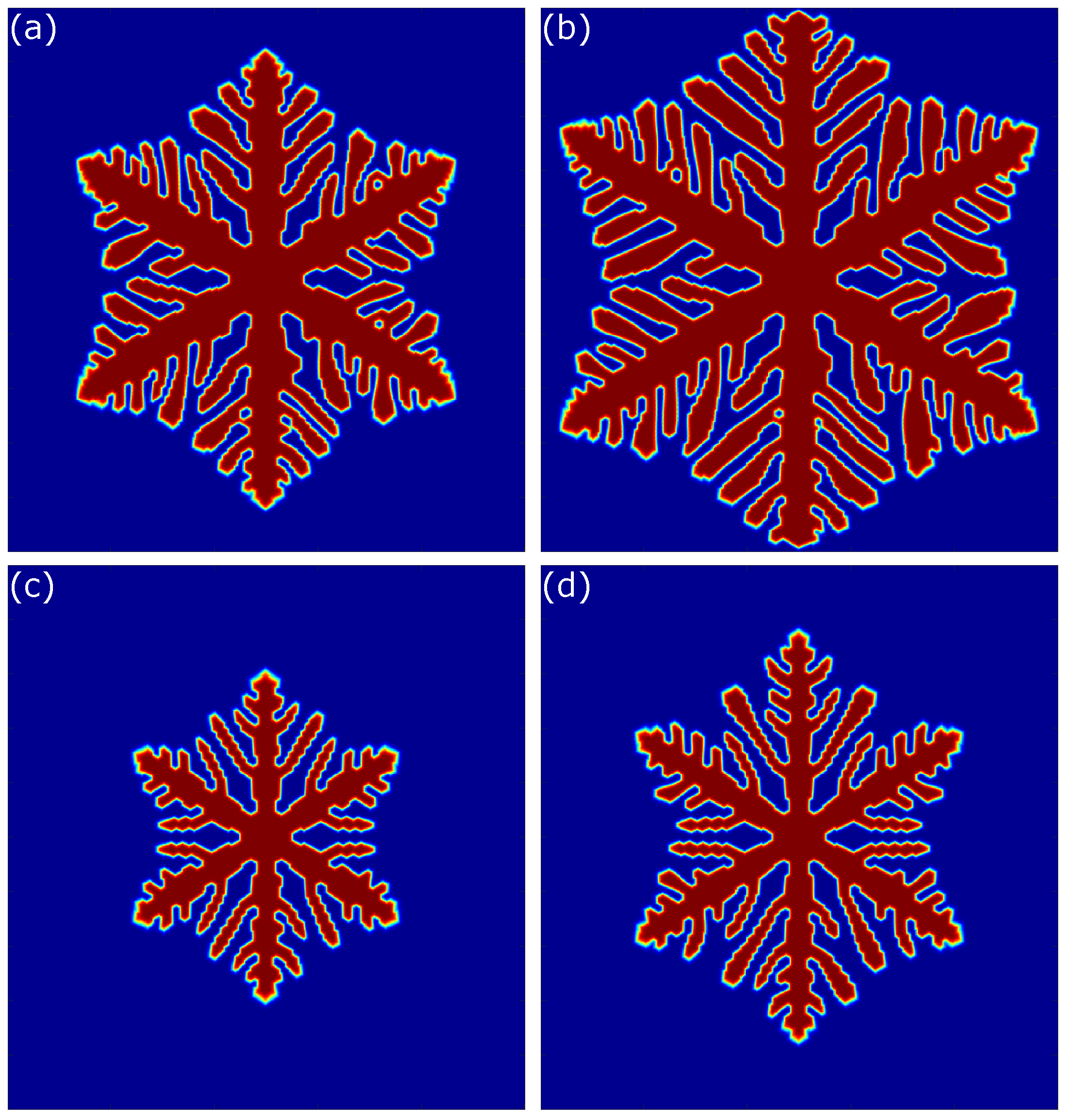
5.1.1. Effect of Latent Heat

Two different values of latent heat $K=1.6$ and $K=2.0$ are considered for the comparison of IGA, FEM and FDM. Other parameters are listed in Table 1. The dendrite structures obtained by IGA at two time stages $t=0.28$ and $t=0.36$ are plotted in Figure 4. All the results illustrate that the dendrite morphologies change with latent heat. The six primary dendrites grow along the selected directions. The angle between each primary dendrite and y axis stays at ${60}^{\mathrm{o}}$ since the anisotropy mode is taken as $j=6$ and the initial angle is set to be ${\theta }_0={90}^{\mathrm{o}}$. As we know, latent heat reflects the heat-released energy in the process of phase solidification [58]. With the increase in K, the heat at the front of dendrites accumulates and results in smaller supercooling. Thus, dendrites grow slower and are finer. These phenomena can be easily observed from panels (a) to (b) and panels (c) to (d). For instance, at time $t=0.36$, the morphology in the case of $K=1.6$ (panel (b)) reaches the boundary of the computational domain while it occupies less space and is still far to the boundary in the case of $K=1.6$ (panel (d)).

A similar conclusion can be obtained in cases of FEM and FDM (see Figure 5 and Figure 6). From the structures in Figure 4, Figure 5 and Figure 6, we notice that the interfaces obtained by IGA and FEM are much smoother than those from FDM. It can be explained that the NURBS-based IGA, as well as FEM, can capture the feathers of interfaces easily and accurately, even across mesh boundaries.

A comparison of computational efficiency among the three methods is presented in

Table 2. CPU time consumed by IGA, FEM and FDM for the problem with $K=2.0$ (unit of CPU time: minute).

Method	Mesh	Processor Number	CPU Time
The proposed method	$256\times 256$	4	8.2
	$256\times 256$	16	2.7
	$256\times 256$	64	0.9
	$512\times 512$	4	37
	$512\times 512$	16	12
	$512\times 512$	64	4.2
	$1024\times 1024$	4	160
	$1024\times 1024$	16	54
	$1024\times 1024$	64	19
FEM	$256\times 256$	4	9.1
	$256\times 256$	16	2.9
	$256\times 256$	64	1.1
	$512\times 512$	4	44
	$512\times 512$	16	15
	$512\times 512$	64	4.8
	$1024\times 1024$	4	173
	$1024\times 1024$	16	62
	$1024\times 1024$	64	23
FDM	$512\times 512$	1	52

. The same numerical case $K=2.0$ is carried out by all of them. $\mathsf{\Delta }t=0.000025$ and total time step $N=7200$ is chosen by FDM due to the computational stability in the case of $512\times 512$ grids. Constant time step $\mathsf{\Delta }t=0.001$ and total time step $N=360$ are used by IGA and FEM in the case of $512\times 512$ elements. The numbers of elements used by IGA and FEM, for example, $256\times 256$, $512\times 512$ and $1024\times 1024$, are chosen for comparison. The implementation of IGA is carried out by an in-house developed message passing interface (MPI) Fortran code, while the FEM code is from the open-source, parallel object-oriented C++ finite element framework, MOOSE (Multiphysics Object Oriented Simulation Environment) [59]. Both of them are implemented in the same high-performance cluster (Intel(R) Xeon(R) CPU E5-2692 v2 2.20 GHz). The Matlab code of FDM for the solidification can be found in reference [60]. From Table 2, the computational efficiencies of IGA and FEM are almost at the same level, while FDM shows high efficiency as expected. Indeed, FDM takes less computational effort. However, it is not easy to deal with a complicated computational domain and apply a boundary condition. In the following section, a simulation of a solidification problem in a droplet-like geometry is implemented by IGA.

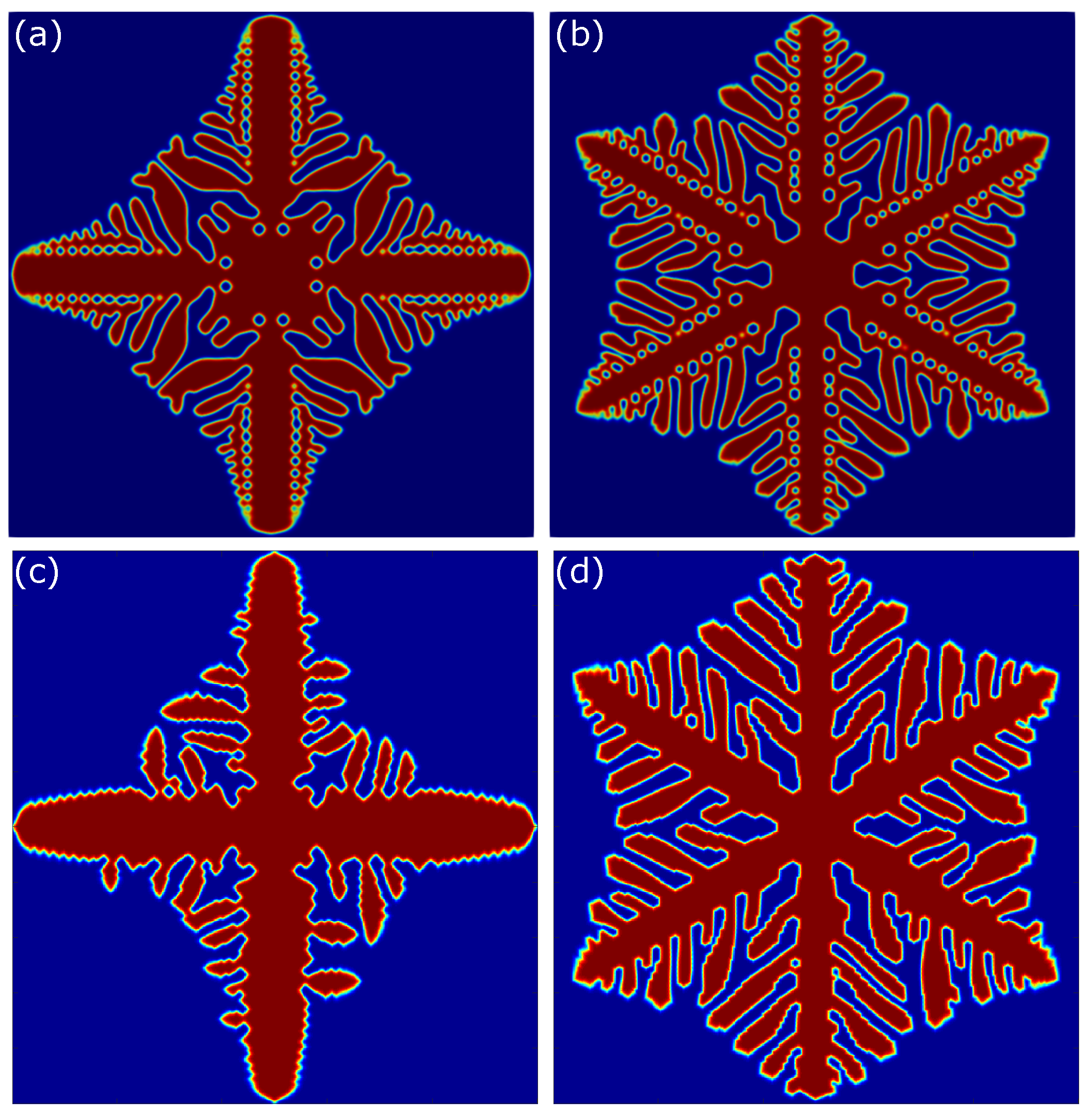
5.1.2. Effect of Anisotropy Mode

The anisotropy mode directly affects the shape of dendrite growth and determines the number of primary dendrites. In this subsection, two different modes $j=4$ and $j=6$ are tested, and the corresponding results computed by IGA and FDM are compared in Figure 7.

Four primary branches are obtained both by IGA and FDM, as shown in Figure 7a,c, in the case of mode $j=4$, while six branches are obtained by IGA and FDM in Figure 7b,d in the case of mode $j=6$. As the anisotropy mode increases, the number of primary dendrites increases. From the results plotted in Figure 7, the anisotropy mode significantly affects the subsequent morphologies of dendrites and plays an important role in the physical and chemical properties of crystals. Comparing the lengths of the main branches, we can conclude that the growth rates of the primary crystals keep the same in both numerical methods when mode $j=4$ is chosen. However, the second branch grows faster when $j=6$ is adopted. Although similar morphologies of crystals are obtained by both IGA and FDM, we still notice that the interfaces from IGA are more smooth than those from FDM. This may be explained by the intrinsic merit of NURBS basis functions.

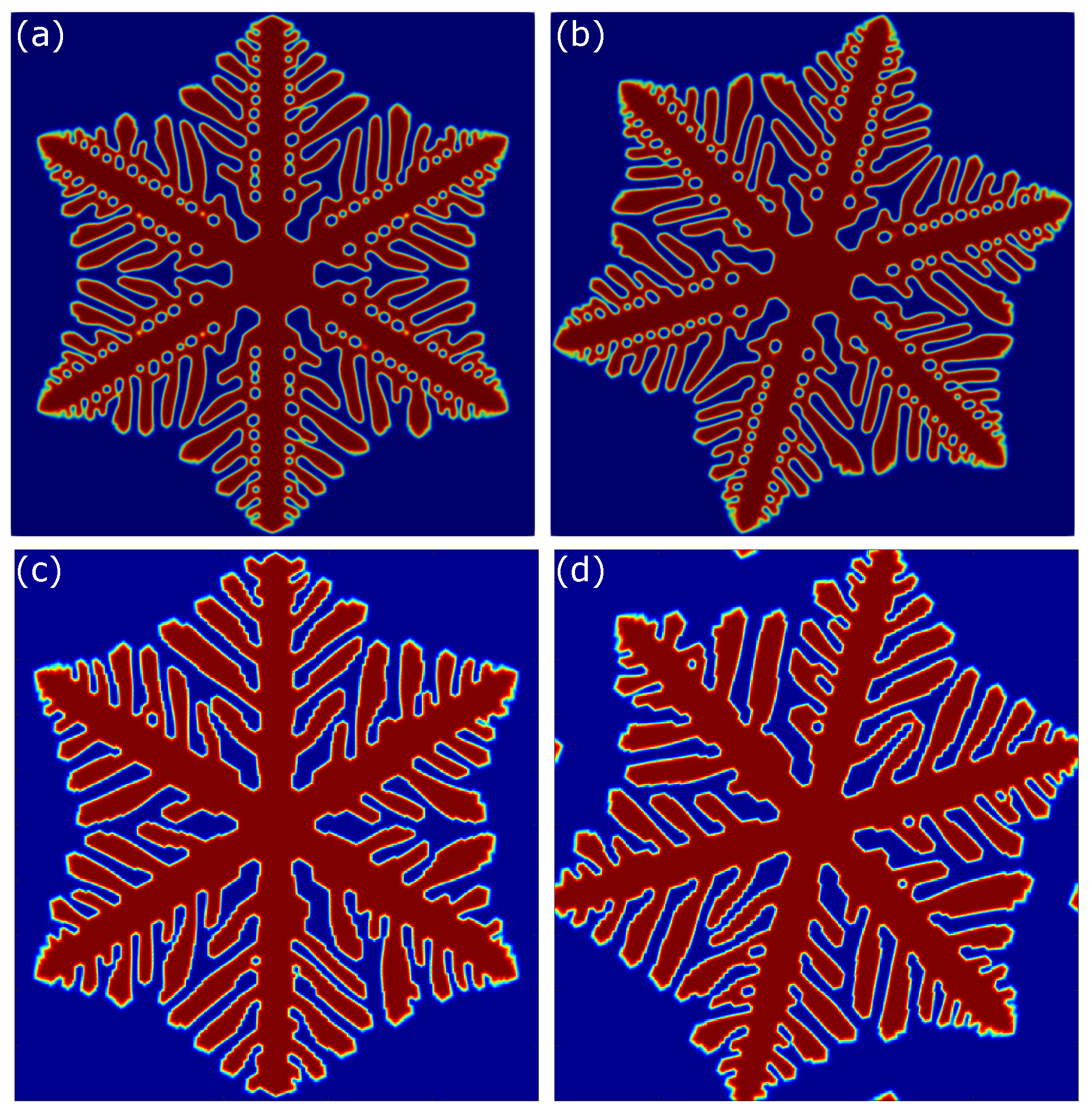
5.1.3. Effect of Initial Angle

The physical meaning of the initial angle ${\theta }_0$ is the orientation of the anisotropy axis, and it determines the growth angles of consequent crystals from primary dendrites. The effect of the initial angle on crystal orientation can be observed easily in numerical simulation. As shown in Figure 8, two different angles ${\theta }_0={90}^{\circ }$ and ${\theta }_0={135}^{\circ }$ are observed. Panels in the first and second rows in Figure 8 demonstrate the structures obtained from IGA and FDM, respectively.

Comparing with panels (a) and (b), as well as panels (c) and (d), the change in initial angle only affects the orientation of the primary dendrite. The shapes and structures of the formed dendrites should remain the same theoretically. However, the two morphologies in panels (a) and (b) are not exactly identical when structures in panel (b) rotate ${45}^{\circ }$ in a clockwise direction. Similar situations can also be found in panels (c) and (d). There are several tiny differences in front of the interfaces and sub-branches. These differences result from the errors in numerical computations, initial condition settings, the meshing generation in the interface front and so on.

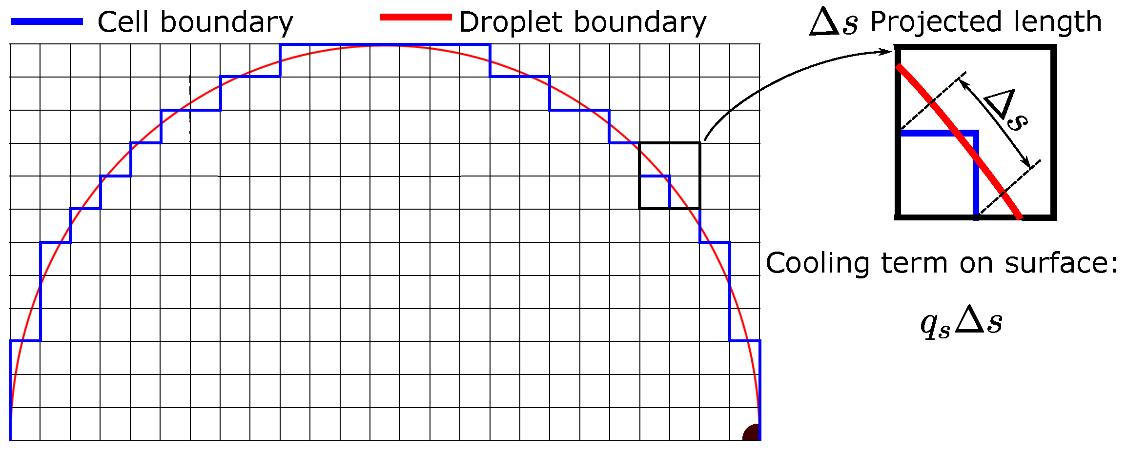
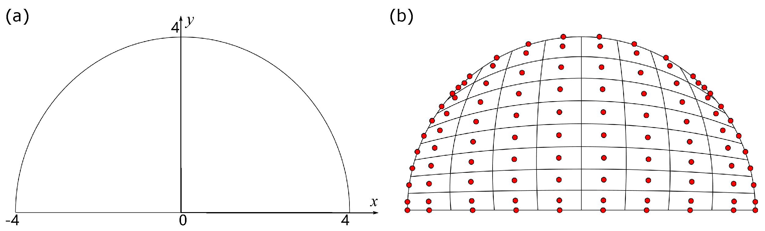
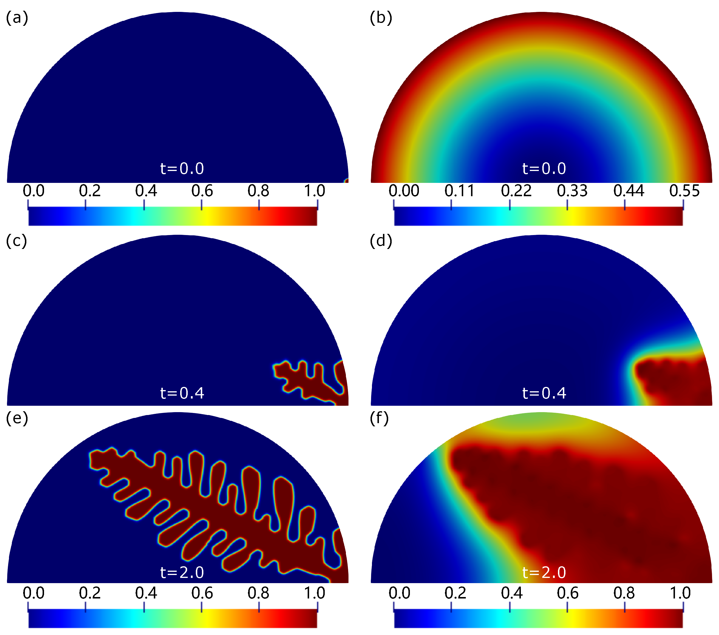
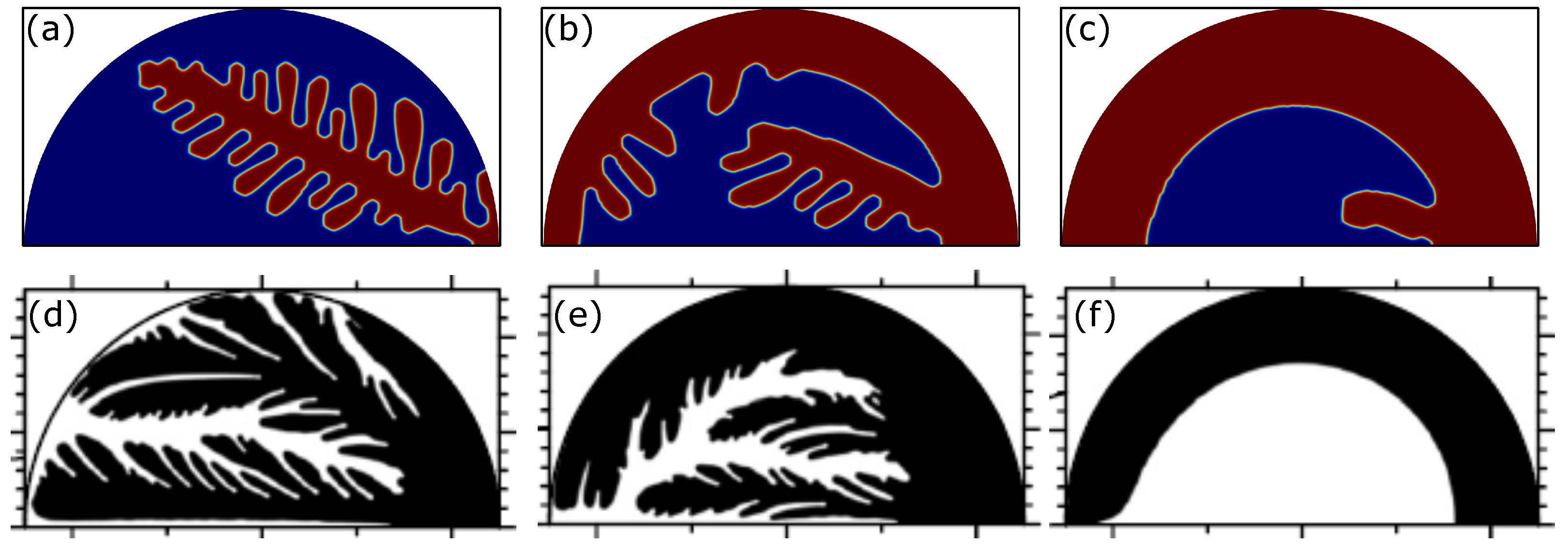
5.2. Dendrite Growth under Different Cooling Rates on Droplet Surface

We study the effect of different supercooling rates on the crystallization in a melt droplet. Panel (a) of Figure 9 illustrates the geometry of the melt droplet, and panel (b) shows an example of an IGA mesh representation of the semicircular domain. We can see that the boundary of the droplet is exactly represented by a few IGA elements. A uniform computational mesh composed of $512\times 256$${\mathcal{C}}^2$ elements is used in all the following simulations.

In order to describe the supercooling on the drop surface, an extra term is added to Equation (8). Then, the updated formula for temperature evolution is expressed as

$${\displaystyle \frac{\partial T}{\partial t}}=\nabla ·\nabla T+K{\displaystyle \frac{\partial \varphi }{\partial t}}-c\mathcal{H}\left(d\right)$$

(35)

where c is the dimensionless undercooling rate, and $\mathcal{H}(·)$ is the Heaviside function that takes the value of 1 on the boundary and 0 in the remaining region. d is the distance to the boundary surface. In this sense, any complex interior/exterior boundary conditions and supercooling rate can be applied freely by adopting the least squares method [61]. Three different cooling rates, namely $c=0$, $c={10}^2$ and $c={10}^5$, are studied. All other parameters take the values listed in Table 1. The initial crystal is circular with a radius 0.1, and its center is located at point (4,0), as shown in Figure 10a. The initial temperature in the droplet is expressed by $T_0=1-(-7.785d_0^2+2289)/2289$, where $d_0$ is the distance to the droplet center and is given in Figure 10b.

Initially, we study the dendrite growth without supercooling at the surface, which keeps the rate at $c=0$. Due to the faster temperature gradient inside the droplet than that on the surface, the main branch grows faster in the interior region than the other one (see panels (c) and (e) in Figure 10). As the energy is released in front of the interface during the solidification process, the temperature increases gradually in the solid phase (see panels (d) and (f) in Figure 10). See Video S1 in the Supplemental Material for an illustration, and a detailed description of the movie can be found in Appendix B.

Then, we increase the cooling rate to $c={10}^2$ and keep other parameters the same. The crystallization on the boundary surface shows faster growth than that in the case of $c=0$ at time $t=0.2$, by comparing the two panels of Figure 10c and Figure 11a. Furthermore, we notice that the first branch on the surface grows faster than that in the interior as time evolves (see panels in Figure 11). Eventually, the surface growth stops when the dendrite reaches the other end of the semicircle, and its second sub-branches grow toward the droplet center due to the temperature gradient. The corresponding illustration can be found in the Supplemental Material (Video S2).

We further increase the supercooling rate up to $c={10}^5$ and obtain the dendrite and temperature evolution, as illustrated in Figure 12 and Video S3 in the Supplemental Material. Unlike the co-growth of the dendrite on the surface and in the interior, the crystallization growth is almost along the boundary, and no sub-branch is developed except the other main branch at the very beginning ($t=0.2$). When the dendrite on the surface reaches the other end of the semicircle, it also gradually grows toward the center. As expected, the distribution of temperature on the surface tends to be zero because of the rapid cooling speed (see panel (f) of Figure 12).

According to the findings in the three cases, we can conclude that the dendrite growth can be controlled by the undercooling rate. With the increase in rate, the growth on the surface is dominant, and eventually, only surface growth exists when an extreme rate is reached. This observation matches the numerical results from reference [5] and experimental observations in [52]. As shown in Figure 13, the dendrite growth towards the interior is dominant without the boundary supercooling (panels (a) and (d)). With small cooling rates on the surface, growth along the boundary and towards the inside co-exists (panels (b) and (e)). When a much bigger rate is applied to the boundary surface, the solidification only happens along the circumferential direction initially and then develops uniformly towards the center of the droplet (panels (c) and (f)).

6. Conclusions

The phase-field method has been commonly embedded in FDM to describe the dendrite growth during solidification. As we know, FDM is hard to deal with regarding problems with irregular boundaries. In order to overcome this bottleneck, we present an IGA-based computational framework for 2D dendrite growth, which can be easily extended for 3D simulation. Numerical studies show that the performance of IGA is comparable to that of FEM and is even better than FDM in some cases. In addition, an improved way to deal with irregular boundary supercooling is also illustrated, and numerical findings agree well with other researchers’ work and experimental observations. In this work, the geometry of the droplet is not complex but is typical. In the case of extremely complex geometry, no matter how complicated the boundary is, we just need to identify it through the Heaviside function $\mathcal{H}(·)$. We believe that IGA creates another way to study dendrite growth and other related fields in material science.

References

1. Zhou, J.; Qi, L. Numerical simulation of liquid-solid extrusion process based on the mechanical model coupled with solidification. Adv. Mech. Eng. 2013, 5, 932348. [Google Scholar] [CrossRef] [PubMed]
2. Ferreira, A.F.; de Castro, J.A.; Ferreira, I.L. 2D phase-field simulation of the directional solidification process. Appl. Mech. Mater. 2015, 704, 17–21. [Google Scholar] [CrossRef]
3. Amar, M.B.; Pomeau, Y. Theory of dendritic growth in a weakly undercooled melt. Europhys. Lett. 1986, 2, 307. [Google Scholar] [CrossRef]
4. Rappaz, M.; Gandin, C.-A. Probabilistic modelling of microstructure formation in solidification processes. Acta Metall. Mater. 1993, 41, 345–360. [Google Scholar] [CrossRef]
5. Miura, H.; Yokoyama, E.; Nagashima, K.; Tsukamoto, K.; Srivastava, A. Phase-field simulation for crystallization of a highly supercooled forsterite-chondrule melt droplet. J. Appl. Phys. 2010, 108, 114912. [Google Scholar] [CrossRef]
6. Chen, L.Q. Phase-field models for microstructure evolution. Annu. Rev. Mater. Res. 2002, 32, 113–140. [Google Scholar] [CrossRef] [Green Version]
7. Militzer, M. Phase field modeling of microstructure evolution in steels. Curr. Opin. Solid State Mater. Sci. 2011, 15, 106–115. [Google Scholar] [CrossRef]
8. Elder, K.R.; Provatas, N.; Berry, J.; Stefanovic, P.; Grant, M. Phase-field crystal modeling and classical density functional theory of freezing. Phys. Rev. B 2007, 75, 064107. [Google Scholar] [CrossRef] [Green Version]
9. Chen, L.; Chen, J.; Lebensohn, R.A.; Ji, Y.Z.; Heo, T.W.; Bhattacharyya, S.; Chang, K.; Mathaudhu, S.; Liu, Z.K.; Chen, L.-Q. An integrated fast fourier transform-based phase-field and crystal plasticity approach to model recrystallization of three dimensional polycrystals. Comput. Meth. Appl. Mech. Eng. 2015, 285, 829–848. [Google Scholar] [CrossRef]
10. Jeong, J.-H.; Goldenfeld, N.; Dantzig, J.A. Phase field model for three-dimensional dendritic growth with fluid flow. Phys. Rev. E 2001, 64, 041602. [Google Scholar] [CrossRef] [PubMed]
11. Karma, A.; Kessler, D.A.; Levine, H. Phase-field model of mode III dynamic fracture. Phys. Rev. Lett. 2001, 87, 045501. [Google Scholar] [CrossRef] [Green Version]
12. Borden, M.J.; Hughes, T.J.R.; Landis, C.M.; Verhoosel, C.V. A higher-order phase-field model for brittle fracture: Formulation and analysis within the isogeometric analysis framework. Comput. Meth. Appl. Mech. Eng. 2014, 273, 100–118. [Google Scholar] [CrossRef]
13. Zheng, X.; Babaee, H.; Dong, S.; Chryssostomidis, C.; Karniadakis, G. A phase-field method for 3D simulation of two-phase heat transfer. Int. J. Heat Mass Transf. 2015, 82, 282–298. [Google Scholar] [CrossRef] [Green Version]
14. Zhang, X.; Kang, J.; Guo, Z.; Han, Q. Effect of the forced flow on the permeability of dendritic networks: A study using phase-field-lattice Boltzmann method. Int. J. Heat Mass Transf. 2019, 131, 196–205. [Google Scholar] [CrossRef]
15. Sedaghatkish, A.; Sadeghiseraji, J.; Jamalabadi, M.Y.A. Numerical simulation of magnetic nanofluid (MNF) film boiling on cylindrical heated magnet using phase field method. Int. J. Heat Mass Transf. 2020, 152, 119546. [Google Scholar] [CrossRef]
16. Zhu, H.; Zhang, Z.; Xu, J.; Ren, Y.; Zhu, Z.; Xu, K.; Wang, Z.; Wang, C. A numerical study of picosecond laser micro-grooving of single crystalline germanium: Mechanism discussion and process simulation. J. Manuf. Process. 2021, 69, 351–367. [Google Scholar] [CrossRef]
17. Zhu, H.; Wang, C.; Mao, S.; Zhang, Z.; Zhao, D.; Xu, K.; Liu, Y.; Li, L.; Zhou, J. Localized and effcient machining of germanium based on the auto-coupling between picosecond laser irradiation and electrochemical dissolution: Mechanism validation and surface characterization. J. Manuf. Process. 2022, 77, 665–677. [Google Scholar] [CrossRef]
18. Bueno, J.; Bona-Casas, C.; Bazilevs, Y.; Gomez, H. Interaction of complex fluids and solids: Theory, algorithms and application to phase-change-driven implosion. Comput. Mech. 2015, 55, 1105–1118. [Google Scholar] [CrossRef]
19. Mokbel, D.; Abels, H.; Aland, S. A phase-field model for fluid–structure interaction. J. Comput. Phys. 2018, 372, 823–840. [Google Scholar] [CrossRef] [Green Version]
20. Frieboes, H.B.; Jin, F.; Chuang, Y.-L.; Wise, S.M.; Lowengrub, J.S.; Cristini, V. Three-dimensional multispecies nonlinear tumor growth-II: Tumor invasion and angiogenesis. J. Theor. Biol. 2010, 264, 1254–1278. [Google Scholar] [CrossRef]
21. Oden, J.T.; Hawkins-Daarud, A.J.; Prudhomme, S. General diffuse-interface theories and an approach to predictive tumor growth modeling. Math. Models Methods Appl. Sci. 2010, 20, 477–517. [Google Scholar] [CrossRef] [Green Version]
22. Oden, J.T.; Prudencio, E.E.; Hawkins-Daarud, A.J. Selection and assessment of phenomenological models of tumor growth. Math. Models Methods Appl. Sci. 2013, 23, 1309–1338. [Google Scholar] [CrossRef]
23. Moure, A.; Gomez, H. Computational model for amoeboid motion: Coupling membrane and cytosol dynamics. Phys. Rev. E 2016, 94, 042423. [Google Scholar] [CrossRef] [PubMed] [Green Version]
24. Xu, J.; Vilanova, G.; Gomez, H. A mathematical model coupling tumor growth and angiogenesis. PLoS ONE 2016, 53, 449–464. [Google Scholar] [CrossRef] [Green Version]
25. Xu, J.; Vilanova, G.; Gomez, H. Full-scale, three-dimensional simulation of early-stage tumor growth: The onset of malignancy. Comput. Meth. Appl. Mech. Eng. 2016, 314, 126–146. [Google Scholar] [CrossRef]
26. Xue, S.L.; Li, B.; Feng, X.Q.; Gao, H.J. A non-equilibrium thermodynamic model for tumor extracellular matrix with enzymatic degradation. J. Mech. Phys. Solids 2017, 104, 32–56. [Google Scholar] [CrossRef]
27. Feng, X.Q. Advances in tumor biomechanics. J. Med. Biomech. 2019, 34, 115–120. [Google Scholar]
28. Xu, J.; Vilanova, G.; Gomez, H. Phase-field model of vascular tumor growth: Three-dimensional geometry of the vascular network and integration with imaging data. Comput. Meth. Appl. Mech. Eng. 2020, 359, 112648. [Google Scholar] [CrossRef]
29. Pismen, L.M. Patterns and Interfaces in Dissipative Dynamics; Springer Science & Business Media: Berlin/Heidelberg, Germany, 2006. [Google Scholar]
30. Steinbach, I. Phase-field models in materials science. Model. Simul. Mater. Sci. Eng. 2009, 17, 073001. [Google Scholar] [CrossRef]
31. Moelans, N.; Blanpain, B.; Wollants, P. An introduction to phase-field modeling of microstructure evolution. Calphad 2008, 32, 268–294. [Google Scholar] [CrossRef]
32. Kobayashi, R.; Warren, J.A.; Carter, W.C. Vector-valued phase field model for crystallization and grain boundary formation. Phys. D Nonlinear Phenom. 1998, 119, 415–423. [Google Scholar] [CrossRef]
33. Warren, J.A.; Boettinger, W.J. Prediction of dendritic growth and microsegregation patterns in a binary alloy using the phase-field method. Acta Metall. Mater. 1995, 43, 689–703. [Google Scholar] [CrossRef]
34. Trivedi, R.; Kurz, W. Dendritic growth. Int. Mater. Rev. 1994, 39, 49–74. [Google Scholar] [CrossRef]
35. Hughes, T.J.; Cottrell, J.A.; Bazilevs, Y. Isogeometric analysis: CAD, finite elements, NURBS, exact geometry and mesh refinement. Comput. Meth. Appl. Mech. Eng. 2005, 194, 4135–4195. [Google Scholar] [CrossRef] [Green Version]
36. Shojaee, S.; Ghelichi, M.; Izadpanah, E. Combination of isogeometric analysis and extended finite element in linear crack analysis. Struct. Eng. Mech. 2013, 48, 125–150. [Google Scholar] [CrossRef]
37. Singh, S.; Singh, I.V.; Bhardwaj, G.; Mishra, B. A Bézier extraction based XIGA approach for three-dimensional crack simulations. Adv. Eng. Softw. 2018, 125, 55–93. [Google Scholar] [CrossRef]
38. Chen, L.; Lingen, E.J.; de Borst, R. Adaptive hierarchical refinement of NURBS in cohesive fracture analysis. Int. J. Numer. Methods Eng. 2017, 112, 2151–2173. [Google Scholar] [CrossRef] [Green Version]
39. Luu, A.-T.; Kim, N.-I.; Lee, J. NURBS-based isogeometric vibration analysis of generally laminated deep curved beams with variable curvature. Compos. Struct. 2015, 119, 150–165. [Google Scholar] [CrossRef]
40. Valizadeh, N.; Natarajan, S.; Gonzalez-Estrada, O.A.; Rabczuk, T.; Bui, T.Q.; Bordas, S.P. NURBS-based finite element analysis of functionally graded plates: Static bending, vibration, buckling and flutter. Compos. Struct. 2013, 99, 309–326. [Google Scholar] [CrossRef] [Green Version]
41. Faroughi, S.; Shafei, E.; Rabczuk, T. Multi-patch NURBS formulation for anisotropic variable angle tow composite plates. Compos. Struct. 2020, 241, 11196. [Google Scholar]
42. Xu, G.; Mourrain, B.; Duvigneau, R.; Galligo, A. A new error assessment method in isogeometric analysis of 2D heat conduction problems. Adv. Sci. Lett. 2012, 10, 508–512. [Google Scholar] [CrossRef] [Green Version]
43. Gómez, H.; Calo, V.M.; Bazilevs, Y.; Hughes, T.J.R. Isogeometric analysis of the Cahn–Hilliard phase-field model. Comput. Meth. Appl. Mech. Eng. 2008, 197, 4333–4352. [Google Scholar] [CrossRef]
44. Gomez, H.; Hughes, T.J.R.; Nogueira, X.; Calo, V.M. Isogeometric analysis of the isothermal Navier–Stokes–Korteweg equations. Comput. Meth. Appl. Mech. Eng. 2010, 199, 1828–1840. [Google Scholar] [CrossRef]
45. Nagy, A.P.; Abdalla, M.M.; Gürdal, Z. Isogeometric sizing and shape optimisation of beam structures. Comput. Meth. Appl. Mech. Eng. 2010, 199, 1216–1230. [Google Scholar] [CrossRef]
46. Manh, N.D.; Evgrafov, A.; Gersborg, A.R.; Gravesen, J. Isogeometric shape optimization of vibrating membranes. Comput. Meth. Appl. Mech. Eng. 2011, 200, 1343–1353. [Google Scholar] [CrossRef] [Green Version]
47. Xu, G.; Mourrain, B.; Duvigneau, R.; Galligo, A. Parameterization of computational domain in isogeometric analysis: Methods and comparison. Comput. Meth. Appl. Mech. Eng. 2011, 200, 2021–2031. [Google Scholar] [CrossRef] [Green Version]
48. Ashour, M.; Valizadeh, N.; Rabczuk, T. Isogeometric analysis for a phase-field constrained optimization problem of morphological evolution of vesicles in electrical fields. Comput. Meth. Appl. Mech. Eng. 2021, 377, 113669. [Google Scholar] [CrossRef]
49. Dhote, R.P.; Gomez, H.; Melnik, R.N.V.; Zu, J. Isogeometric analysis of a dynamic thermo-mechanical phase-field model applied to shape memory alloys. Comput. Mech. 2014, 53, 1235–1250. [Google Scholar] [CrossRef]
50. Gomez, H.; Bures, M.; Moure, A. A review on computational modelling of phase-transition problems. Philos. Trans. R. Soc. A 2019, 377, 20180203. [Google Scholar] [CrossRef] [PubMed] [Green Version]
51. Valizadeh, N.; Rabczuk, T. Isogeometric analysis for phase-field models of geometric PDEs and high-order PDEs on stationary and evolving surfaces. Comput. Meth. Appl. Mech. Eng. 2019, 351, 599–642. [Google Scholar] [CrossRef]
52. Tsukamoto, K.; Kobatake, H.; Nagashima, K.; Satoh, H.; Yurimoto, H. Crystallization of cosmic materials in microgravity. Lunar Planet. Sci. 2001, 32, 1846. [Google Scholar]
53. Kobayashi, R. A brief introduction to phase field method. AIP Conf. Proc. 2010, 1270, 282–291. [Google Scholar]
54. Takaki, T. Phase-field modeling and simulations of dendrite growth. ISIJ Int. 2014, 54, 437–444. [Google Scholar] [CrossRef] [Green Version]
55. Koric, S.; Thomas, B.G.; Voller, V.R. Enhanced latent heat method to incorporate superheat effects into fixed-grid multiphysics simulations. Numer. Heat Transf. Part B 2010, 57, 396–413. [Google Scholar] [CrossRef]
56. de Boor, C. Package for Calculating with B-Splines. SIAM J. Numer. Anal. 1977, 14, 441–472. [Google Scholar] [CrossRef]
57. Jansen, K.E.; Whiting, C.H.; Hulbert, G.M. A generalized-method for integrating the filtered Navier-Stokes equations with a stabilized finite element method. Comput. Meth. Appl. Mech. Eng. 2000, 190, 305–319. [Google Scholar] [CrossRef]
58. Tiaden, J.; Nestler, B.; Diepers, H.-J.; Steinbach, I. The multiphase-field model with an integrated concept for modelling solute diffusion. Phys. D Nonlinear Phenom. 1998, 115, 73–86. [Google Scholar] [CrossRef]
59. Permann, C.J.; Gaston, D.R.; Andrš, D.; Carlsen, R.W.; Kong, F.; Lindsay, A.D.; Miller, J.M.; Peterson, J.W.; Slaughter, A.E.; Stogner, R.H.; et al. MOOSE: Enabling massively parallel multiphysics simulation. SoftwareX 2020, 11, 100430. [Google Scholar] [CrossRef]
60. Sanal, R. Numerical simulation of dendritic crystal growth using phase field method and investigating the effects of different physical parameter on the growth of the dendrite. arXiv 2014, 1412, 3197. [Google Scholar]
61. Nguyen, V.P.; Anitescu, C.; Bordas, S.P.; Rabczuk, T. Isogeometric analysis: An overview and computer implementation aspects. Math. Comput. Simulat. 2015, 117, 89–116. [Google Scholar] [CrossRef]
Figure 1. Special strategy for applying supercooling boundary conditions on droplet surface in FDM [5]. Δ s is the projected effective length, and q s is the normal component to the droplet boundary.
Metals 12 01836 g001
Figure 2. Chemical free energy of the phase-field equation for solidification. When temperature is less than melting temperature, namely m > 0 , the interfacial phase tends to be a solid phase, which suggests dendrite growth. The opposite situation can be concluded if m < 0 . In the case of m = 0 , the interface might not move. Definition of element domains in IGA. Physical elemental domain Ω e (Top), elemental domain Ω ^ e in parametric space (bottom left) and Gaussian integration domain Ω ¯ e (bottom right).
Metals 12 01836 g002
Figure 3. Definition of element domains in IGA. Physical elemental domain Ω e (Top), elemental domain Ω ^ e in parametric space (Bottom left) and Gaussian integration domain Ω ¯ e (Bottom right).
Metals 12 01836 g003
Figure 4. Dendrite structures obtained by IGA with K = 1.6 and K = 2.0 at different time stages. The first row shows the morphologies of dendrites in the case of K = 1.6 at t = 0.28 (a) and t = 0.36 (b). The second row shows those in the case of K = 2 at t = 0.28 (c) and t = 0.36 (d).
Metals 12 01836 g004
Figure 5. Dendrite structures obtained by FEM with K = 1.6 and K = 2.0 at different time stages. The first row shows the morphologies of dendrites in the case of K = 1.6 at t = 0.28 (a) and t = 0.36 (b). The second row shows those in the case of K = 2 at t = 0.28 (c) and t = 0.36 (d).
Metals 12 01836 g005
Figure 6. Dendrite structures obtained by FDM with K = 1.6 and K = 2.0 at different time stages. The first row shows the morphologies of dendrites in the case of K = 1.6 at t = 0.28 (a) and t = 0.36 (b). The second row shows those in the case of K = 2 at t = 0.28 (c) and t = 0.36 (d).
Metals 12 01836 g006
Figure 7. Simulations of dendrite growth with different anisotropy modes solved by IGA (panels (a,b)) and FDM (panels (c,d)). The morphologies of dendrites in panels (a,c) are obtained by using j = 4 , and those morphologies in panels (b,d) are for j = 6 at the same time t = 0.36 .
Metals 12 01836 g007
Figure 8. Simulation results of dendrite growth affected by initial angle. The morphologies of dendrites with θ 0 = 90 and θ 0 = 135 are compared at t = 0.36 . (a,b) The morphologies of dendrites with θ 0 = 90 and θ 0 = 135 from IGA. (c,d) Under the same conditions, the morphologies of dendrites from FDM.
Metals 12 01836 g008
Figure 9. Geometry of the melt droplet (a) and an example of IGA mesh (b). The domain is discretized by 8 × 8 elements just for viewing purposes. The corresponding control points are indicated by solid red circles.
Metals 12 01836 g009
Figure 10. Evolution of dendrite structures and temperature at different stages in the case of c = 0 . Initial nucleus (a) and distribution of normalized temperature within the domain (b); dendrite structures at t = 0.4 (c) and t = 2.0 (e), and temperature evolution at t = 0.4 (d) and t = 2.0 (f).
Metals 12 01836 g010
Figure 11. Evolution of dendrite structures and temperature at different stages in the case of c = 10 2 . Initial nucleus (a) and distribution of normalized temperature within the domain (b); Dendrite structures at t = 0.6 (c) and t = 2.0 (e), and temperature evolution at t = 0.6 (d) and t = 2.0 (f).
Metals 12 01836 g011
Figure 12. Evolution of dendrite structures and temperature at different stages in the case of c = 10 5 . Initial nucleus (a) and distribution of normalized temperature within the domain (b); dendrite structures at t = 0.6 (c) and t = 2.0 (e), and temperature evolution at t = 0.6 (d) and t = 2.0 (f).
Metals 12 01836 g012
Figure 13. Evolution of dendrite structures at different stages in cases of various cooling rates. Panels (ac) and (df) are obtained from the proposed method and FDM in reference [5], respectively. Reproduced with permission from Miura et al. [5] (df).
Metals 12 01836 g013