Calibration of the Flow Curve Up to Large Strain Range by Incremental Sheet Forming Coupled with FEM Simulation

Abstract

Conventionally, a stress–strain curve for sheet materials is defined by the uniaxial tensile test; however, it is limited by the necking phenomena. The stress–strain curve in the post-necking range is determined using common hardening equations, such as the Swift or Voce equation. Nevertheless, the accuracy of this flow curve in the extrapolation range is questionable. In this study, the inverse method using incremental sheet forming coupled with FEM simulation was used to calibrate the stress–strain curve up to a large strain range. In the incremental sheet forming experiment, the forming force was monitored in the whole process until fracture. Then, FEM simulation by ABAQUS/Explicit was performed using the incremental stress–strain curve, accompanied by Hill’s 1948 yield behavior. The incremental stress–strain curve was calculated using the $\mathsf{\beta }$ parameter, which was systematically assigned to adjust the trial stress at each strain increment of the FEM process. The correct incremental stress–strain curve was determined when the force prediction was in good agreement with the experiment.

1. Introduction

An important goal of the metal forming processes is the production of defect-free parts with the desired microstructure and properties. This can be achieved by improving the design and calculation methods and better controlling the parameter of the deformation processes, which should be based on a deeper knowledge of the phenomena that accompany a material’s deformation and the relation between the deformed material’s properties and the condition of deformation. Three significant characteristics are required to study sheet metal forming processes: the stress–strain curve, yielding behavior, and flow rule theory. Conventionally, the stress–strain curve is experimentally determined by the uniaxial tensile test. This test provides the relation between stress and strain until the fracture occurs. However, in real manufacturing, many forming processes exceed the uniform strain achieved in the uniaxial tensile test. Therefore, metallic materials’ post-necking behavior describes the relation between stress and strain beyond the uniform strain, which has recently been widely studied.

The initial effective stress–strain curve can be determined using a well-known hardening function to match the experimental true stress–strain curve at the pre-necking range. In previous studies, several hardening functions have been used for this purpose, for example, the Hollomon equation [1], Swift equation [2], or a combination equation [3]. In addition, many methods have been proposed to better identify the flow stresses of sheet metals beyond the neck or post-necking behavior. Pham et al. [4,5] introduced a strain-hardening model called the Kim–Tuan model to improve the post-necking prediction accuracy for aluminum alloy. Coppieters et al. [6] described a more consistent equation for the post-necking range, including the work hardening rate at the maximum tensile force point in the equation. In their research, the digital image correlation (DIC) method was used to characterize more detailed information about the material behavior after necking occurrences during the uniaxial tensile test. Saboori et al. [7] presented two different methods, a weighted average method and a new hardening function, to extend the true stress–true strain curve after necking. The two methods resulted in similar post-necking curves for the different materials, with the consideration that the new hardening function could be used for more complicated hardening laws. Moreover, the simulation results exhibited good accuracy using the proposed methods. Recently, Pham et al. [8] presented a new procedure in which the experimental data obtained from the uniaxial tensile test and the measured forming limit at a plane strain tension mode are adopted in the curve fitting procedure for calibrating the parameters of different hardening laws. The measured forming limit curve ($FL{C}_0$) is introduced in the cost function of the fitting to provide an additional constraint for the hardening parameters in large strain ranges. The results indicated that the flow curves predicted by the Kim–Tuan hardening model effectively matched the experimental data obtained from uniaxial tensile tests.

On the other hand, the stress–strain curve until a large strain can be easily identified using commercial finite element analysis (FEA) software in which experimental data of tensile load and displacement of the gauge length are required. Therefore, an FE model is developed in either a self-developed FEA program or commercial software to analyze the tensile specimen. The effective stress–strain curve trace is iteratively adjusted step-by-step to reduce the difference between the simulated and experimental load–displacement curves to a pre-set tolerance level. In particular, two concerns influence the computational cost: the initial effective stress–strain curve used in the first analysis and the adjustment method used to modify the effective stress–strain curve.

Rather than the initial effective stress–strain curve, the adjustment method strongly affects the convergence rate of iteration regardless of whether a post-necking hardening function is required separately. Joun et al. [9] reported that the current true stress at the current average axial true strain was corrected by a ratio of the measured axial load over the computed axial load. While implementing such a step-by-step iterative optimization procedure during the FEA is effective, implementing it is a general-purpose commercial finite element program is difficult. In contrast, Zhao et al. [10] successfully determined the effective stress for each 0.05 increment of effective strain. Their research de-fined an upper bound (modeling by the linear curve tangential to the last data point) and a lower bound (modeling by the flat curve extended horizontally from the last data point) and divided the stress values between the upper and lower bounds into 15 increments. A total of 16 feasible stress values were tried to simulate the tensile test, and thus, the strategy generates a large number of computations. More efficiently, Mei et al. [11] proposed an inverse modeling method to determine the hardening curve to large strains. The post-necking hardening behavior of the material was determined by an FE-based inverse modeling procedure that used the raw data from the tensile test. The inverse method was then compared with some classical hardening models. Furthermore, the biaxial tensile test at elevated temperatures was performed to evaluate the applicability of the inverse method further. Alternatively, Kweon et al. [12] described a methodology to determine the true stress–strain curve of stainless steels in the full range of strain from a typical tensile test. In their method, the true stress and strain values were directly converted from engineering stress and strain data before necking. In contrast, a true stress–strain equation was determined by iteratively conducting FEA using the information at the necking and fracture points after necking. This method is intrinsically simple to use and reduces iterations. More efficiently, Pham et al. [13] presented a hybrid method incorporating the curve fitting method and inverse finite element analysis to identify the Kim–Tuan hardening model’s parameters over large strain ranges. Here, the curve fitting method enforces the identified hardening law’s accuracy in the pre-necking range. Simultaneously, the inverse finite element analysis method maintains the goodness of the post-necking prediction.

The inverse calculation coupled with FEM simulation of the uniaxial tensile test (UT test) only provides the stress–strain curve up to necking or fracture strains, observed during the UT test. However, during the forming process such as the bulge test, incremental sheet forming (ISF), and so on, the strain value induced during the process is larger than the fracture strain observed during the UT test. Therefore, the stress–strain curve, far beyond the UT limit, can be predicted and corrected more accurately by using the inverse method combining FEM and forming process with large deformation.

Conversely, several studies related to incremental sheet forming (ISF) with a single-point tool were reviewed by Behera et al. [14]. The ISF deformation mechanisms involve stretching and shear in the plane perpendicular to the tool direction, with shear in the plane parallel to the tool direction. The strains increase on successive laps, and the most significant component of strain is shear parallel to the tool direction [15]. To evaluate the strain evolution in the ISF process, experimental and numerical studies have been performed by Do et al. [16]. The strain value in ISF was very high compared to that in tensile tests or conventional press forming. A similar result was obtained by Mirnia et al. [17], wherein the stress–strain curve was fitted by the Swift equation. With a large strain value in ISF, the calibration for the accurate stress–strain curve is questionable; however, the forming force is measurable and can be used for calibration purposes.

Several studies have been reported on the forming forces in ISF because it explains the deformation mechanics and the forming process. Duflou et al. [18] designed an experimental system for measuring three force components to evaluate the effect of the process parameters on the forming forces: the vertical step size, tool diameter, and wall angle. They also considered the effects of the sheet thickness and lubrication. Aerens et al. [19] observed that the forming force proportionally increased with the wall angles. A similar trend was observed for the tool diameter and vertical step size [20]. Moreover, the tool rotation and lubrication had no considerable influence on the forming forces.

Furthermore, the forming force prediction by FEM simulation has been extensively studied. Flores et al. [21] concluded that the yield locus and hardening behavior are very important for force prediction by FEM models. The mixed hardening model showed better force prediction compared to Von Mises or Hill constitutive laws with isotropic hardening. Henrard et al. [22] used different codes (ABAQUS and Lagamine) to simulate the ISF process with different constitutive hardening models and element types. The mixed isotropic–kinematic hardening model accompanied by brick element offers the best force prediction, but its computation time is extremely long. Concurrently, the shell element can afford significant time consumption reduction with good prediction accuracy.

In this study, the inverse method using ISF coupled with FEM simulation was used to define the stress–strain curve up to a large strain range for the Al5052-O materials. First, the experiments to measure the forming force in ISF of the AL5052-O sheet were performed. Thus, the FEM simulation by ABAQUS/Explicit was performed using the incremental stress–strain curve, accompanied by Hill’s 1948 yield behavior. The incremental stress–strain curve was calculated using the $\mathsf{\beta }$ parameter, which was systematically assigned to adjust the trial stress at each strain increment of the FEM process. The correct incremental stress–strain curve was determined when the force prediction was in good agreement with the experimental data. Moreover, the mechanical properties of the 0.8 mm thick AL5052-O sheet material in a uniform elongation range were evaluated.

2. Experiments

2.1. Material Properties

To obtain the flow stress–strain relation for the AL5052-O sheet, a series of uniaxial tensile tests were performed following the ASTM-8 standard (Figure 1a) procedure at a constant tensile speed of 10 mm/min with a gauge length of 50 mm. To increase the accuracy and reduce the effect of the cutting process on the surface of the specimens, the laser cutting method was used to prepare the specimens.

To evaluate the anisotropic plasticity behavior of the AL5052-O sheet, uniaxial tensile tests were conducted in three different directions with respect to the rolling direction, 0°, 45°, and 90°. The material properties of the AL5052-O sheet are summarized in

Table 1. Mechanical properties of Al5052-O.

Direction	0$°$	$45°$	$90°$
Young’s modulus [GPa]	73.2	71.2	74.1
Yield stress [MPa]	183.3	172.5	173.6
Ultimate tensile strength [MPa]	229.8	216.6	220.1
Elongation [%]	11.0	13.6	10.5
R-value	0.758	0.646	0.863
KT	131.580	124.809	124.268
m	0.271	0.278	0.251
c	61.163	75.433	69.521

, including Young’s modulus (E), ultimate tensile strength (UTS), and elongation ($\Delta \mathrm{l}$). The initial yield stress and material anisotropy R-values are also reported for the three directions (${\sigma }_0,{\sigma }_{45}$,${\sigma }_{90}, R_0, R_{45}, R_{90}$). Figure 1b displays the true stress–true strain curves of the studied material for the three different orientations. Through the differences in the initial yield stresses and plastic strain ratios for the three different orientations, Table 1 demonstrates that the AL5052-O sheet is an anisotropic material. Furthermore, Figure 1 clearly shows that the flow curves in different directions are represented by different curvatures, exhibiting distinct tensile strength, elongation, and necking area.

Conventionally, either the Swift equation (power law) or the Voce equation (exponent law) can be used to describe the strain hardening behavior of sheet metals. However, the use of these equations to predict the post-necking behavior of sheet metals remains questionable, as indicated by Coppieters et al. [6]. Therefore, in this research, the Kim–Tuan model, is proposed to model the stress–strain relation of the AL5052-O sheet material and successfully describe the material behavior on both sides of the necking point: pre-necking and post-necking behaviors. The formulation of the Kim–Tuan (K–T) hardening model is expressed as follows:

$$\mathsf{\sigma }={\sigma }_0+K_T{\left(\epsilon +{\epsilon }_0\right)}^m\left(1-ex{p}^{-c\epsilon }\right)$$

(1)

where K_T, m, and c are the parameters of the proposed equation, and m is a dependent parameter calculated as follows:

$$m=\frac{{\sigma }^{*}}{{\sigma }^{*}-{\sigma }_0}\left({\epsilon }^{*}+{\epsilon }_0\right)$$

(2)

Here, (${\epsilon }_0$,${\sigma }_0$) represents the initial yield point of the true stress–true strain curve and (${\epsilon }^{*}$,${\sigma }^{*}$) the plastic strain and stress according to the maximum tensile force point. The parameter $m$ is a dependent parameter whose value is independent of other parameter values. Therefore, the parameters K_T and c in the Kim–Tuan model are calculated using the curve fitting tool, which is available on some optimization packages such as Excel or MATLAB. The Kim–Tuan equation can be easily reduced to the Swift equation when ${\sigma }_0$ is ignored and c is infinity. In addition, this equation can be simplified to the Voce equation when the parameter $m$ is zero.

Figure 2 exhibits the curve fitting results for the AL5052-O sheets using three different strain hardening models: the Swift power law, Voce exponent law, and Kim–Tuan equation. In the three models, the Kim–Tuan hardening model enforces the work hardening rate or the slope of the stress–strain curve ($\mathrm{d}\mathsf{\sigma }/\mathrm{d}\mathsf{\epsilon }$) at the maximum tensile force point of the fitted curve equal to that of the experiment. Due to this, the proposed equation is advantageous for studying the post-necking behavior of sheet metals without requiring any other plasticity properties, except the stress–strain data from the uniaxial tensile test.

2.2. ISF Experiment

The AL5052-O sheet part is formed by incremental sheet forming, as shown in Figure 3a. In this test, we employed the two-wing star toolpath, as shown in Figure 3b. The other forming parameters include a tool diameter of 10 mm, vertical step $\Delta \mathrm{Z}$ of 0.25 mm, feed rate of 200 mm/minute, and MoS2 lubrication to eliminate the sliding friction between the tool and the sheet. The forming speed was selected at a low value to get the strain rate as low as the uniaxial tensile test. A specimen with a size of 140 mm × 60 mm is clamped on the straight-groove die, which was made from SKD11 steel to support the blank shoulder. Position A and B are higher than the initial sheet plane, which means the tool is not in contact with the sheet metal at these positions. The tool moves in the order of A-O-B with a downward distance $\Delta \mathrm{Z}$ in the center O to finish the first depth increment. For the second depth increment, the movement follows the order of B-O-A. The process is repeated in the next depth increment until a fracture occurs.

As shown in Figure 3c, when the tool continuously descends to the center position and causes the area to fracture, the test stops immediately.

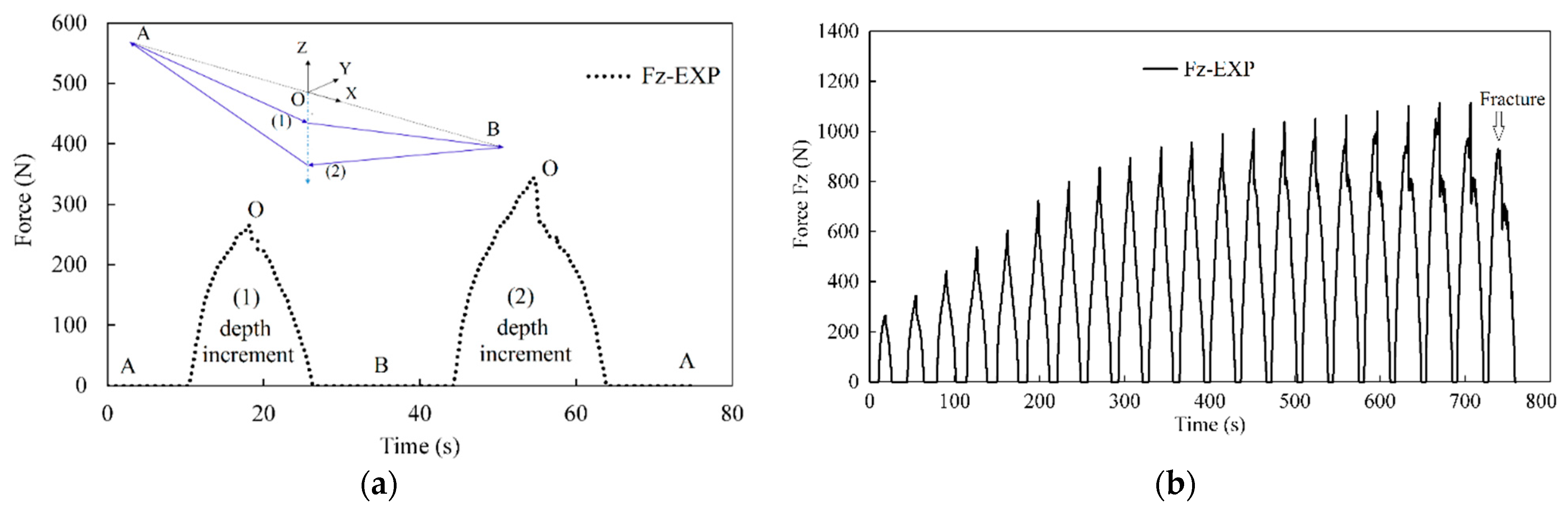
2.3. Forming Force Measurement

The forming force was measured experimentally in many previous studies. In this study, forming force was measured by an LRL load cell. The tool goes from the initial position A (not in contact with the sheet) and gradually goes to position B in the first depth increment. The forming force increases from 0 up to the maximum value at O and decreases to 0 when the tool goes up to point B. In the second depth increment, the trend is similar to the maximum force occurring at the center position O, as shown in Figure 4a.

The forming force was monitored for the entire forming process until the occurrence of a fracture, as shown in Figure 4b. At the next depth increment, the forming force exhibited the same trend with a maximum value at the center position, and the maximum force value increased with the forming depth. At the 21st depth increment, fracture occurred, as shown in Figure 3c. Thus, the forming force was dramatically reduced, and the measurement process was stopped. The experiment was repeated three times, and the fracture occurred at the 21st depth increment in all of them, the maximum forming depth of which is 5.25 mm.

3. Finite Element Simulation

3.1. The Associated Flow Rule with Mixed Hardening

An AL5052-O sheet was used for this study. It is undeniable that AL5052-O is an anisotropic material owing to both the tensile strength mean and the anisotropic plastic ratio [23]. From this perspective, anisotropic functions should be used to derive the plastic work behavior of this material; thus, Hill’s 1948 yield criteria were considered to describe the plastic work behaviors of the studied material [24]. The parameters of yield function (F, G, H, and N) were calculated based on the strain terms ($R_0, R_{45}, R_{90}$). Further formulation of Hill’s quadratic function can be found in [24].

Table 2. Parameters of material AL5052-O.

Yield Function Hill48
F	G	H	N
0.4996	0.5688	0.4312	1.2244

shows the parameters of these functions.

The yield criterion, as a function of all state variables, can be written in a generic form as

$$F\left(\sigma , \alpha , {\sigma }^Y\right)=f_y\left(\sigma -\alpha \right)-{\sigma }^Y\left(p\right)=0,$$

(3)

where $f_y\left(\sigma -\alpha \right)$ is a continuously differentiable yield function and $\alpha$ is a back-stress tensor in the kinematic hardening model; if $\alpha$ is ignored, the yield criterion returns to isotropic hardening model. In addition, $p$ is the equivalent plastic strain, and ${\sigma }^Y\left(p\right)$ is the work hardening rule, which is generally represented using the Swift, Voce, or Kim–Tuan equation.

The evolution of the back-stress tensor is modeled based on the nonlinear kinematic hardening theory of the so-called Armstrong–Frederick model (AF model):

$$d\alpha =\left(\frac{C}{f_p}\eta -\gamma \alpha \right)dp$$

(4)

Here, tensor $\eta$ is defined as $\eta =\left(\sigma -\alpha \right)$; C and $\gamma$ are material constants. For the AL5052-O material, C and $\gamma$ are 1118.26 MPa and 23.694, respectively.

Hill’s 1948 anisotropic yield function in the plane stress condition is

$$f_y=\sqrt{\left(G+H\right){\eta }_x^2+\left(F+H\right){\eta }_y^2-2H{\eta }_x{\eta }_y+2N{\eta }_{xy}^2 }$$

(5)

where ${\sigma }^Y$ is the yield stress in the reference direction and F, G, H, and N are constant characteristics of the anisotropy, defined as follows:

$$G=\frac{1}{1+R_0};H=\frac{R_0}{1+R_0};F=\frac{R_0}{\left(1+R_0\right)R_{90}}; N=\frac{\left(1+2R_{45}\right)\left(R_0+R_{90}\right)}{2\left(1+R_0\right)R_{90}}$$

(6)

3.2. Calibration of Stress–Strain Curve Up to Large Strain Range

ABAQUS version 6.14 was used for the elastic-plastic simulations of the incremental forming process. The finite element model is shown in Figure 5. The full model was considered to ensure the correct results because the symmetry condition does not correctly describe the mechanical deformation of the sheet during the forming process. The AL5052-O sheet was meshed by a square-shaped S4R type with a size of 0.5 mm and was integrated by Gauss integration with nine points in the through-thickness direction. The outer boundary of the sheet is constrained by six degrees of freedom. The fixed die was modeled as a discrete rigid body and meshed by the R3D4 element. The tool with a diameter of 10 mm was modeled as analytically rigid. In addition, to respond to the inertia effect, the tool is given the same mass in the simulation as the actual one.

The physical time cannot be used in the dynamic explicit simulations because using such a large time step leads to an enormous simulation time. In practice, determining a virtual simulation time is essential to guarantee good agreement between the simulation and experiment results. Simultaneously, the virtual simulation time could not be too small so as to avoid introducing the non-physical dynamic effects into the derived simulation results. After several tries, the virtual simulation time is set to 0.1 s for the one forming step.

In the ISF process, lubricants are usually used to reduce friction. To match the friction condition with the real experiment, the friction coefficient between forming tool and sheet is set to 0.05. [25] In addition, a VUMAT subroutine was developed accompanying Hill’s 1948 yield function in the two-wing star test simulation for the AL5052-O sheet. The VUMAT code for ABAQUS/EXPLICIT software consists of a semi-explicit method for the stress update algorithm. Moreover, the VUHARD was also used for expressing the plastic stress–strain behavior by adopting the Kim–Tuan hardening law.

In the first simulation, the stress–strain curve in the uniform deformation range obtained from the uniaxial tensile test was inputted in the FEM simulation. The forming force prediction by FEM was compared to the experimental results, as shown in Figure 6a. The equivalent plastic strain PEEQ for the element in the center area of the sheet was also plotted in the same graph. The time scaling factor was used to equalize the step time in FEM with that of the experiment. In the first and second depth increments, the PEEQ value was in the pre-necking range, the force prediction by FEM and by the experiment was in good agreement. However, from the third depth increment (Figure 6b), the PEEQ value was higher than 0.1, and the maximum force prediction by FEM (426 N) was lower than that of the experiment (442 N). This result shows that the stress value was higher than the value at the end of the uniform elongation at the large range of the equivalent plastic strain.

To define the stress–strain curve in the post-necking range, an inverse method by ISF coupled with FEM simulation was used. The principle of this method is to select a correct stress value at each trial strain value, whose results are sensitive to the prediction force in each FEM simulation (Figure 7). The numerical results are then compared with the experimental measurements. The trial stress value is iteratively adjusted and simulated again until the difference between the numerical and experimental curves is minimized. The advantage of this method is the possibility of selecting nonhomogeneous stress and strain states close to the states reached during the process to be simulated. In this study, at each strain increment value of 0.05, the trial stress value with incremental factor β was attempted for the different values at 0, ±0.02, ±0.04, ±0.06, ±0.08, and ±0.1, which, although the value of beta tends to be positive due to the hardening behavior of metallic materials, for the softening behavior of composite materials [26] and some metal materials at high temperatures, the value of $\mathsf{\beta }$ can be negative [27]. The best agreement result between FEM and the experiment was selected, and the corresponding trial stress value was defined. The process was repeated, as shown in the flow chart in Figure 8, until the final step when the fracture occurred.

Figure 6b shows that the stress value was higher than the value at the end of uniform elongation in the large range of equivalent plastic strain. Therefore, the stress–strain data with increment strain of (${\epsilon }_u+0.05$) and the trial stress value with positive incremental factor $\mathsf{\beta }$ were used for the next FEM simulation. The force prediction results with different incremental factor $\mathsf{\beta }$ for the first three forming steps are shown in Figure 9a. The maximum force prediction in the 3rd step proportionally increased with the increment factor$\mathsf{\beta }$. Compared to the maximum experimental force, the prediction result for the case factor $\mathsf{\beta }$ of 0.04 was the best agreement. Similar processes with a trial strain of 0.05 and different trial stress increment $\mathsf{\beta }$ were performed to calibrate the forming force for the next forming step until fracture. In each trial strain value, one trial stress increment factor $\mathsf{\beta }$ was defined, and the trial stress–trial strain curve in a large strain range up to 1.0 was plotted, as shown in Figure 9b. Moreover, note that this trial stress–trial strain curve is close to the curve obtained by the Kim–Tuan hardening equation in a large strain range.

The force prediction by the FEM model with the best-fitted trial stress–trial strain curve and FEM model with the Voce hardening equation was performed. In these simulations, the previously defined forming limit curve at fracture (FLCF) [12] was applied to predict the fracture occurrence. The forming limit curve at fracture for AA5052-O was illustrated as the following equation, where ${\epsilon }_1$ and ${\epsilon }_2$ are the major and minor strains, respectively.

$${\epsilon }_1=-1.04{\epsilon }_2+1.24$$

(7)

During the simulation process, the fracture occurred in an element when its FLDCRT value, which is defined by the ratio of the major calculated strains (${\epsilon }_{1cal}$) and the FLCF values (${\epsilon }_{1FLCF}$) at the same point for the minor strains (${\epsilon }_2$), reached the unit value.

In both simulations, if the FLDCRT value for elements in the center area was over the unit first, the elements were deleted (Figure 10a). However, the FEM model with the best-fitted trial stress–trial strain curve predicted the fracture at the 21st depth increment (forming depth is 5.25 mm), while the FEM model with the Voce hardening equation showed the fracture at the 20th depth increment (forming depth is 5 mm). Thus, the FEM model with the best-fitted trial stress–trial strain provided the correct prediction of fracture depth and the FEM model with the Voce hardening equation predicted the fracture earlier than the experiment.

The forming force prediction by both FEM models for each forming depth increment was compared to the experimental measurement and are shown in Figure 10b. As shown in the magnified view for the 15th and 20th depth increments, the results of the FEM model with the best-fitted trial stress–trial strain curve matched the experiment’s result, while the FEM model using the Voce hardening equation underestimated the forming force. The measured maximum forming force at 15th and 20th increments for the experiment, FEM using the fitted curve, and FEM using Voce are organized in

Table 3. Measured maximum forming force at 15th and 20th increments.

Increment	Experimental (N)	FEM Using the Fitted Curve (N)	FEM Using Voce Curve (N)
15th	1050.3	1065.73	956.39
20th	1095.97	1104.38	766.37

. It can be clearly seen that at the 15th and 20th increments, the errors between the FEM model with the best-fitted trial stress–trial strain curve and experiment are 1.4% and 0.76%, while the errors between the FEM model using the Voce hardening equation and experiment are 8.9% and 30.1%.

4. Conclusions

The inverse method using the ISF process coupled with FEM simulation was used in this study which gives a new strategy to define the stress–strain curve up to a large strain range. First, the experiment to measure the forming force in ISF was performed. Then, the FEM simulation by ABAQUS/Explicit was performed using the incremental stress–strain curve, accompanied by Hill’s 1948 yield behavior. The incremental stress–strain curve was selected at each strain increment of 0.05 to simulate the forming process. Each corrected trial stress was selected for each trial strain value when the force prediction was in good agreement with the experiment. Using this method, the best-fitted trial stress–trial strain curve was calibrated up to large strain ranges, compared to the tensile test or conventional press forming process.

At the same time, it is worth noting that the Kim–Tuan hardening equation has a good ability of prediction for stress–strain in a large strain range because the hardening rate at the point of maximum tensile force is considered.

Without loss of generality, the hardening behavior of sheet metals correlates well to the forming force required to deform the sheet during ISF processes. This work draws an early step on the calibration material model by using the ISF process. Future works should be conducted to identify material models for different automotive sheet metals to verify the robustness of the proposed method. At the same time, the effects of process parameters, such as tool diameter, tool speed rate, and so on, on the calibrated results should be investigated in the forthcoming paper.

References

1. Hollomon, J.H. Tensile deformation. Trans. Metall. Soc. AIME 1945, 162, 268–290. [Google Scholar]
2. Swift, H.W. Plastic instability under plane stress. J. Mech. Phys. Solids 1952, 1, 1–18. [Google Scholar] [CrossRef]
3. Sung, J.H.; Kim, J.H.; Wagoner, R.H. A plastic constitutive equation incorporating strain, strain-rate, and temperature. Int. J. Plast. 2010, 26, 1746–1771. [Google Scholar] [CrossRef]
4. Pham, Q.T.; Kim, Y.S. Identification of the plastic deformation characteristics of AL5052-O sheet based on the non-associated flow rule. Met. Mater. Int. 2017, 23, 254–263. [Google Scholar] [CrossRef]
5. Pham, Q.T.; Lee, B.H.; Park, K.C.; Kim, Y.S. Influence of the post-necking prediction of hardening law on the theoretical forming limit curve of aluminium sheets. Int. J. Mech. Sci. 2018, 140, 521–536. [Google Scholar] [CrossRef]
6. Coppieters, S.; Kuwabara, T. Identification of Post-Necking Hardening Phenomena in Ductile Sheet Metal. Exp. Mech. 2014, 54, 1355–1371. [Google Scholar] [CrossRef] [Green Version]
7. Saboori, M.; Champliaud, H.; Gholipour, J.; Gakwaya, A.; Savoie, J.; Wanjara, P. Extension of flow stress–strain curves of aerospace alloys after necking. Int. J. Adv. Manf. Technol. 2016, 83, 313–323. [Google Scholar] [CrossRef]
8. Pham, Q.T.; Lee, M.G.; Kim, Y.S. New procedure for determining the strain hardening behavior of sheet metals at large strains using the curve fitting method. Mech. Mater. 2021, 154, 103729. [Google Scholar] [CrossRef]
9. Joun, M.S.; Eom, J.G.; Lee, M.C. A new method for acquiring true stress–strain curves over a large range of strains using a tensile test and finite element method. Mech. Mat. 2008, 40, 586–593. [Google Scholar] [CrossRef]
10. Zhao, K.; Wang, L.; Chang, Y.; Yan, J. Identification of post-necking stress–strain curve for sheet metals by inverse method. Mech. Mat. 2016, 92, 107–118. [Google Scholar] [CrossRef]
11. Mei, H.; Lang, L.H.; Liu, K.N.; Yang, X.Q. Evaluation Study on Iterative Inverse Modeling Procedure for Determining Post-Necking Hardening Behavior of Sheet Metal at Elevated Temperature. Metals 2018, 8, 1044. [Google Scholar] [CrossRef] [Green Version]
12. Kweon, H.D.; Kim, J.W.; Song, O.; Oh, D. Determination of true stress-strain curve of type 304 and 316 stainless steels using a typical tensile test and finite element analysis. Nucl. Eng. Technol. 2021, 53, 647–656. [Google Scholar] [CrossRef]
13. Pham, Q.T.; Thoi, T.N.; Ha, J.J.; Kim, Y.S. Hybrid fitting-numerical method for determining strain-hardening behavior of sheet metals. Mech Mater. 2021, 161, 104031. [Google Scholar] [CrossRef]
14. Behera, A.K.; Sousa, R.A.; Ingarao, G.; Oleksik, V. Single point incremental forming: An assessment of the progress and technology trends from 2005 to 2015. J. Manuf. Process. 2017, 27, 37–62. [Google Scholar] [CrossRef] [Green Version]
15. Ai, S.; Long, H. A review on material fracture mechanism in incremental sheet forming. Int. J. Adv. Manuf. Technol. 2019, 104, 33–61. [Google Scholar] [CrossRef] [Green Version]
16. Do, V.C.; Pham, Q.T.; Kim, Y.S. Identification of forming limit curve at fracture in incremental sheet forming. Int. J. Adv. Manuf. Technol. 2017, 92, 4445–4455. [Google Scholar] [CrossRef]
17. Mirnia, M.J.; Shamsari, M. Numerical prediction of failure in single point incremental forming using a phenomenological ductile fracture criterion. J. Mater. Proc. Technol. 2017, 244, 17–43. [Google Scholar] [CrossRef]
18. Duflou, J.; Tunckol, Y.; Szekeres, A.; Vanherck, P. Experimental study on force measurements for single point incremental forming. J. Mat. Proc. Technol. 2007, 189, 65–72. [Google Scholar] [CrossRef]
19. Aerens, R.; Eyckens, P.; Van Bael, A.; Duflou, J.R. Force prediction for single point incremental forming deduced from experimental and FEM observations. Int. J. Adv. Manuf. Technol. 2010, 46, 969–982. [Google Scholar] [CrossRef]
20. Bansal, A.; Lingam, R.; Yadav, S.K.; Reddy, N.V. Prediction of forming forces in single point incremental forming. J. Manuf. Proc. 2017, 28, 486–493. [Google Scholar] [CrossRef]
21. Flores, P.; Duchene, L.; Bouffioux, C.; Lelotte, T.; Henrard, C.; Pernin, N.; Van Bael, A.; He, S.; Duflou, J.; Habraken, A.M. Model identification and FE simulations: Effect of different yield loci and hardening laws in sheet forming. Int. J. Plast. 2007, 23, 420–449. [Google Scholar] [CrossRef] [Green Version]
22. Henrard, C.; Bouffioux, C.; Eychens, P.; Sol, H.; Duflou, J.R.; Van Houtte, P.; Van Bael, A.; Duchene, L.; Habraken, A.M. Forming forces in single point incremental forming: Prediction by finite element simulations, validation and sensitivity. Comput. Mech. 2011, 47, 573–590. [Google Scholar] [CrossRef]
23. Tamura, S.; Sumikawa, S.; Uemori, T.; Hamasaki, H.; Yoshida, F. Experimental Observation of Elasto-Plasticity Behavior of Type 5000 and 6000 Aluminum Alloy Sheets. Mater. Trans. 2011, 52, 868–875. [Google Scholar] [CrossRef] [Green Version]
24. Taherizadeh, A.; Green, D.E.; Ghaei, A.; Whan, Y.J. A non-associated constitutive model with mixed iso-kinematic hardening for finite element simulation of sheet metal forming. Int. J. Plast. 2010, 26, 288–309. [Google Scholar] [CrossRef]
25. Fang, Y.; Lu, B.; Chen, J.; Xu, D.K.; Ou, H. Analytical and experimental investigations on deformation mechanism and fracture behavior in single point incremental forming. J. Mater. Process. Technol. 2014, 214, 1503–1515. [Google Scholar] [CrossRef]
26. Zobeiry, N.; Vaziri, R.; Poursartip, A. Characterization of strain-softening behavior and failure mechanisms of composites under tension and compression. Compos. Part A Appl. Sci. Manuf. 2015, 68, 29–41. [Google Scholar] [CrossRef]
27. Kassner, M.E.; Ermagan, R. Large-Strain Softening of Metals at Elevated Temperatures by Deformation Texture Development. Metals 2021, 11, 1059. [Google Scholar] [CrossRef]
Figure 1. (a) Dimensions of tensile test specimen. (b) Stress–strain curves of the AL5052-O sheet for three different orientations.
Metals 12 00252 g001
Figure 2. Curve fitting results for the AL5052-O sheet in the rolling direction.
Metals 12 00252 g002
Figure 3. (a) Forming set up for incremental sheet forming. (b) Two-wing star toolpath. (c) Fracture happening for the two-wing star toolpath (bottom-up view).
Metals 12 00252 g003
Figure 4. (a) Forming force Fz in the first and second depth increment. (b) Forming force Fz in whole forming process.
Metals 12 00252 g004
Figure 5. FEM model for incremental sheet forming.
Metals 12 00252 g005
Figure 6. (a) The formed part after 3rd depth increment in the FEM. (b) Force Fz prediction by FEM using stress–strain curve in uniform deformation range.
Metals 12 00252 g006
Figure 7. Stress integration scheme at extrapolation range of strain.
Metals 12 00252 g007
Figure 8. Stress integration process.
Metals 12 00252 g008
Figure 9. (a) Force prediction for the first three forming steps with the increment strain of ( ε u + 0.05 ) . (b) Best-fitted trial stress–trial strain in large strain range.
Metals 12 00252 g009
Figure 10. (a) Fracture prediction by FEM with the best-fitted trial stress–trial strain curve. (b) Comparison of the experimental force and force prediction by FEM with different hardening equations.
Metals 12 00252 g010