Assessment of the Generalization Ability of the ASTM E900-15 Embrittlement Trend Curve by Means of Monte Carlo Cross-Validation

Abstract

The standard ASTM E900-15 provides an analytical expression to determine the transition temperature shift exhibited by Charpy V-notch data at 41-J for irradiated pressure vessel materials as a function of the variables copper, nickel, phosphorus, manganese, irradiation temperature, neutron fluence, and product form. The 26 free parameters included in this embrittlement correlation were fitted through maximum likelihood estimation using the PLOTTER—BASELINE database, which contains 1878 observations from commercial power reactors. The complexity of this model, derived from its high number of free parameters, invites a consideration of the possible existence of overfitting. The undeniable goal of a good predictive model is to generalize well from the training data that was used to fit its free parameters to new data from the problem domain. Overfitting takes place when a model, due to its high complexity, is able to learn not only the signal but also the noise in the training data to the extent that it negatively impacts the performance of the model on new data. This paper proposes the resampling method of Monte Carlo cross-validation to estimate the putative overfitting level of the ASTM E900-15 predictive model. This methodology is general and can be employed with any predictive model. After 5000 iterations of Monte Carlo cross-validation, large training and test datasets (7,035,000 and 2,355,000 instances, respectively) were obtained and compared to measure the amount of overfitting. A slightly lower prediction capacity was observed in the test set, both in terms of R² (0.871 vs. 0.877 in the train set) and the RMSE (13.53 °C vs. 13.22 °C in the train set). Besides, strong statistically significant differences, which contrast with the subtle differences observed in R² and RMSE, were obtained both between the means and the variances of the training and test sets. This result, which may seem paradoxical, can be properly interpreted from a correct understanding of the meaning of the p-value in practical terms. In conclusion, the ASTM E900-15 embrittlement trend curve possess good generalization ability and experiences a limited amount of overfitting.

1. Introduction

Several embrittlement trend curves (ETCs) have been developed to predict the ductile to brittle transition temperature shift (TTS), ΔT_41J, of RPV steels [1,2,3,4], which is required when demonstrating the integrity of light water reactors. In 2015, the ASTM Standard E900-15 [3] was approved, providing a correlation to predict the radiation-induced TTS in reactor vessel materials developed from the statistical analysis of a large surveillance database (1878 TTS measurements contained in the so-called BASELINE of the PLOTTER database) obtained in the context of the surveillance programs of nuclear power reactors (test reactors were not considered) from 13 countries (Brazil, Belgium, France, Germany, Italy, Japan, Mexico, The Netherlands, South Korea, Sweden, Switzerland, Taiwan, and the United States). This dataset, therefore, represents the train set used to fit the 26 free parameters of the model. The variables that influence the TTS in this correlation are copper, nickel, phosphorus and manganese contents, irradiation temperature, neutron fluence, as well as the product type (forgings, plates, and SRM plates, and welds) [5]. The form of the correlation is semiempirical because even though the free parameters are fitted using statistical procedures, it includes two major embrittlement terms mechanistically guided that represent the hardening contribution from small microstructural defects and copper-enriched clusters created during irradiation [3].

The predictive correlation provided by ASTM E900-15 [3] is an example of supervised learning, this term being borrowed from the field of Machine Learning. Supervised learning is used whenever a certain outcome (the TTS in this case) is to be obtained from a given input (the set of variables previously mentioned that influence the TTS), and examples of input/output pairs are available (the 1878 observations used to fit the parameters of the formula). It is important to stress that the final goal of any model, either analytical or numerical, is to generalize, i.e., to make accurate predictions for new, never-before-seen data with the same characteristics as the training set [6]. As a matter of fact, complex models can detect subtle patterns in the data but if the training set is noisy, or if it is too small, then the model is likely to detect patterns in the noise itself. Obviously, these patterns will not generalize to new observations, in which case, the model is said to incur overfitting [6,7,8]. Overfitting occurs when the model is too complex relative to the amount and noisiness of the training data. As stated by Chollet [8], the fundamental issue is the tension between optimization and generalization: “Optimization refers to the process of adjusting a model to get the best performance possible on the training data, whereas generalization refers to how well the trained model performs on data it has never seen before. The goal of the game is to get good generalization, of course, but you don’t control generalization; you can only adjust the model based on its training data”.

As mentioned above, the predictive formula proposed by ASTM E900-15 contains 26 free parameters that have been optimized through statistical procedures using all the available information. This number of parameters suggests that it is an analytically complex model, which creates the possibility of overfitting. The objective of this paper is therefore to assess the degree to which the ASTM E900-15 ETC may be overfit by using advanced statistical and data analytics techniques that were not available to the ASTM Committee at the time E900-15 was developed. This paper proposes a simple resampling methodology that enables quantification of the overfitting level of a predictive model. Here, we apply the methodology to the ASTM E900-15 ETC, but it is general and can be applied to any other model. We should note that our objective is restricted to assessing the E900-15 ETC for overfitting; we do not explore the more general question of finding a model that optimally represents the data. As such, our study is restricted to the functional form of the E900-15 ETC.

The remainder of the paper is organized as follows: the ASTM E900-15 ETC [3] and the statistical methods are described in Section 2. Section 3 is devoted to presenting the results of the analysis. Finally, the interpretation and significance of the results is discussed in Section 4.

2. Methods

2.1. The ASTM E900-15 ETC

The mean value of the TTS depends on the variables copper, nickel, phosphorus, manganese, irradiation temperature, neutron fluence, and product form. According to ASTM E900-15 [3], the TTS (in °C) is expressed as the sum of two terms, B and M; see Equation (1). Equations (2) and (3) collectively provide the formula for B, while Equations (4)–(6) collectively provide the formula for M.

$$TTS=B+M$$

(1)

$$B=P{F}_B\frac{5}{9}1.8943 · {10}^{-12}{\mathrm{\Phi }}^{0.5695}{\left(\frac{1.8T+32}{550}\right)}^{-5.47}$$

$${\left(0.09+\frac{P}{0.012}\right)}^{0.216}{\left(1.66+\frac{N{i}^{8.54}}{0.63}\right)}^{0.39}{\left(\frac{Mn}{1.36}\right)}^{0.3}$$

(2)

$$P{F}_B=\left(\begin{array}{c}1.011 for forgings\\ 1.080 for plates and SRM plates\\ 0.919 for welds\end{array}\right)$$

(3)

$$M=P{F}_2\frac{5}{9} max\left[min\left(Cu, 0.28\right)-0.053, 0\right] M_1$$

(4)

$$M_1=max\left\{min\left[113.87 \left(ln\left(\mathrm{\Phi }\right)-ln\left(4.5· {10}^{20}\right)\right), 612.6\right], 0\right\}{\left(\frac{1.8 T+32}{550}\right)}^{-5.45}$$

$${\left(0.1+\frac{P}{0.012}\right)}^{-0.098}{\left(0.168+\frac{N{i}^{0.58}}{0.63}\right)}^{0.73}$$

(5)

$$P{F}_M=\left(\begin{array}{c}0.738 for forgings\\ 0.819 for plates and SRM plates\\ 0.968 for welds\end{array}\right)$$

(6)

In Equations (2), (4), and (5), Cu, Ni, P, and Mn are all expressed in weight percent, neutron fluence Φ is in n/m² (E > 1 MeV) and irradiation temperature T is in °C. A detailed assessment of the conditions to which E900-15 [3] may be applied can be found in [9]. Besides, ASTM E900-15 [3] provides the range of material and irradiation conditions in the BASELINE–PLOTTER database used in the embrittlement correlation. Specifically, Cu < 0.4%, Ni < 1.7%, P < 0.03%, 0.55% < Mn < 2.0%, 255 °C < T < 300 °C, 1 × 10²¹ n/m² < Φ < 2 × 10²⁴ n/m². This analytical model includes 26 free parameters that were fitted using Maximum Likelihood Estimation (MLE) from the data. Relative to the calibration dataset, the model provides unbiased predictions and has a root mean square error (RMSE) of 13.32 °C and a coefficient of determination R² = 0.875 (other alternative correlations based on different datasets are introduced in [5]). ASTM E900-15 [3] adopts expression (7) (W: welds, P: plates and SRM plates, F: forgings) for the standard deviation, SD, which increases along with the predicted value of the TTS:

$$SD=\left[\begin{array}{c}\mathrm{W}:7.681\\ \mathrm{P}:6.593\\ \mathrm{F}: 6.972\end{array}\right]\times TT{S}^{\left[\begin{array}{ccc}\mathrm{W}:0.181& \mathrm{P}:0.163& \mathrm{F}:0.199\end{array}\right]}$$

(7)

The values adopted by ASTM E900-15 [3] for the 26 parameters are collected in

Table 1. Values of the parameters in the ASTM E900-15 [3] ETC; see Equations (2)–(6) (the reader can identify each parameter name in Equations (2)–(6) by comparing the numerical values).

Parameters in “M” (Equations (4)–(6))	Value	Parameters in “B” (Equations (2) and (3))	Value
B_Weld	9.190 × 10−1	CuMAX	2.800 × 10−1
B_Plate	1.080	CuMIN	5.300 × 10−2
B_Forge	1.011	M_Weld	9.680 × 10−1
B_Const	1.894 × 10−12	M_Plate	8.190 × 10−1
B_Exp	5.695 × 10−1	M_Forge	7.380 × 10−1
B_Texp	−5.470	M_slope	1.139 × 102
B_Pconst	9.000 × 10−2	M_Maxslope	6.126 × 102
B_Pexp	2.160 × 10−1	M_lnMinFlu	4.500 × 1020
B_Niconst	1.660	M_Texp	−5.450
B_Niexp1	8.540	M_Pconst	1.000 × 10−1
B_Niexp2	3.900 × 10−1	M_Pexp	−9.800 × 10−2
B_Mnexp	3.000 × 10−1	M_Niconst	1.680 × 10−1
-	-	M_Niexp1	5.800 × 10−1
-	-	M_Niexp2	7.300 × 10−1

. For convenience and to facilitate the assessment included in Section 3.3, a descriptive label has been adopted for each of the parameters in Table 1; the reader can identify each of them without great difficulty by comparing the numerical values in Table 1 with the corresponding ones in Equations (1)–(6).

2.2. Programming Tools

The numerical analysis was developed and evaluated in Python 3, a general-purpose open-source programming language that can be used for a wide variety of applications, including data science. There are several advantages of Python that deserve to be mentioned. For example, Python includes thousands of third-party modules available in the Python Package Index (PyPI). In this sense, this study has used libraries such as Numpy, Pandas, Scikit-Learn, Matplotlib, ScyPy, and Seaborn, among others. Most importantly, Python has an enormous user community that shares code, documentation, tutorials, and examples to help program a solution. For these reasons, it has been repeatedly selected by programmers [10,11] as their favorite programming language.

2.3. The Method of Maximum Likelihood

The Method of Maximum Likelihood (MML), developed in the 1920s by the statistician R. A. Fisher, is one of the preferred methods to obtain a point estimator of a parameter. The central concept in this method is the likelihood function, L [12]. Let X be a random variable with probability distribution f(x;θ), where θ is a single unknown parameter. Let (x₁, x₂, …, x_n) be the observed values of X in a random sample of size n. Then, the likelihood function of the sample is (8):

$$L\left(\theta \right)=f\left(x_1;\theta \right)·f\left(x_2;\theta \right)·\dots ·f\left(x_n;\theta \right)$$

(8)

Therefore, L(θ) represents the probability to obtain the sample values (x₁, x₂, …, x_n). Note that L is now a function of only the unknown parameter θ because (x₁, x₂, …, x_n) are actually observed values of X. The maximum likelihood estimator of θ is the value of θ that maximizes the likelihood function L(θ), i.e., an estimator that maximizes the probability of occurrence of the observed sample values. Mathematically, the maximization of L(θ) corresponds to expression (9) but, in practice, for the sake of simplicity (the log-likelihood maximum is the same as the likelihood maximum but the former is usually easier to optimize since the logarithm of a product is the sum of the logarithms), the logarithm of L(θ) is maximized instead, as in (10):

$$\frac{\partial L\left(\theta \right)}{\partial \theta }=0$$

(9)

$$\frac{\partial lnL\left(\theta \right)}{\partial \theta }=0$$

(10)

The MML can be used in situations involving ‘k’ unknown parameters (θ₁, θ₂, …, θ_k) to estimate, as in this study. In such cases, the maximum likelihood estimators would be found by equating the k (‘k’ being the number of parameters) partial derivatives to zero and solving the resulting system of equations [12]; see Equation (11):

$$\{\begin{array}{c}\frac{\partial L\left({\theta }_1,{\theta }_2, \dots , {\theta }_k\right)}{\partial {\theta }_1}=0\\ \frac{\partial L\left({\theta }_1,{\theta }_2, \dots , {\theta }_k\right)}{\partial {\theta }_2}=0\\ \\ \dots \\ \\ \frac{\partial L\left({\theta }_1,{\theta }_2, \dots , {\theta }_k\right)}{\partial {\theta }_k}=0\end{array}$$

(11)

The MML has prevailed among mathematical statisticians over other alternatives (such as least squares or Bayesian estimation) because of its good statistical properties. As stated by Montgomery and Runger [12], under very general and not restrictive conditions, when the sample size n is large and if $\hat{\mathrm{\Theta }}$ is the maximum likelihood estimator of the parameter θ:

(1)

$\hat{\mathrm{\Theta }}$ is an approximately unbiased estimator for θ;

(2)

The variance of $\hat{\mathrm{\Theta }}$ is nearly as small as the variance that could be obtained with any other estimator;

(3)

$\hat{\mathrm{\Theta }}$ has an approximate normal distribution.

Some complications may arise in using the MML. For example, it may not always be possible to use calculus methods directly to maximize the likelihood function L(θ). Statistical computer programs based on numerical techniques have been specifically developed to solve for the maximum likelihood estimates when no simple closed solutions exist [12]. In this study, the Python library SciPy [13], which provides algorithms for mathematics and statistics, including optimization, has been implemented. The tools in the module scipy.optimize enable minimizing or maximizing objective functions (in this case, the minus logarithm of the likelihood function has been minimized). The numerical method of Nelder–Mead, based on the Simplex algorithm [14,15], which has been proven robust in many applications, has been selected.

2.4. Resampling

Statistical resampling methods are designed to estimate the precision of sample statistics or to validate models. The two most widely preferred methods for estimating the sampling distribution of an estimator are Bootstrapping and Jackknife. Bootstrap uses sampling with replacement to estimate the distribution of the desired target variable. Jackknife works by sequentially deleting one observation in the dataset and repeatedly recalculating the parameter of interest. The main purpose of these methods is to evaluate the variance of an estimator, its confidence interval, and standard error. Cross-validation (CV) methods are aimed at testing the ability of a model to predict new data that was not used to fit the free parameters of the model in order to flag problems like overfitting and to assess how the model will generalize to an independent dataset [16]. K-fold and Monte Carlo cross-validation (MCCV, also known as repeated random sub-sampling validation) techniques are widely used in data analytics [6,7]. Each method has its own advantages and disadvantages. Under K-fold CV, each observation is tested once; however, K-fold only explores a small subset of the possible partitions while MCCV explores a much larger set of combinations. Besides, MCCV defines the distributions of the parameters in the E900-15 equation. For this reason, MCCV has been adopted so that the parameter distributions can be compared to the point-estimates of the parameters provided in ASTM E900-15 [17,18]. This method not only provides an estimation of the sampling distribution of the parameters of the ASTM E900-15 ETC but also provides, at the same time, an unbiased measure of the actual prediction capacity of the model. To reduce variability, a CV analysis typically involves multiple rounds/iterations. Each round consists of randomly splitting the available sample of data into two complementary subsets, namely the training and testing sets. For each split, the model is fit to the training data, and predictive accuracy is assessed using the validation data. Finally, all training data and testing data are respectively combined. Using the common jargon for design of experiments in fields such as biology or economics [19], the train set can be considered as the control group, while the test set can play the role of the treatment group.

2.5. Strategy of the Analysis

The flowchart in Figure 1 describes the strategy followed in the study. The analysis is based on the MCCV method and includes 5000 iterations; in each of them, the dataset, consisting of 1878 observations, has been randomly split into a train set containing 75% of the observations (1407) and a test set with the remaining 25% (471). This train/test separation has been stratified with respect to the product type, that is, the relative proportions of forgings, plates and SRM plates, and welds in the total dataset (1878 instances) has been maintained in the train and test sets. The observations of the train set have been used to recalibrate through MLE the 26 free parameters of the ASTM E900-15 ETC [3]. Subsequently, this recalibrated model has been used to predict the TTS values in both the train and test sets and the results have been stored. After completing the iterative process, a comparison between these sets was conducted in order to identify possible differences.

3. Results

3.1. Descriptive Statistics

Two large datasets were generated after the 5000 iterations of MCCV: a train set with 7,035,000 samples (7,035,000 = 5000 × 1407, where 1407 = 0.75 × 1878) and a test set including 2,355,000 instances (2,355,000 = 5000 × 471, with 471 = 0.25 × 1878). Differences in the distribution of residuals (i.e., the difference between the predicted values of the dependent variable and the observed values) between these sets would be symptomatic of overfitting. The basic statistical scores used to compare the performance in the train and test sets (the mean values of the residuals, the RMSE, and the R² obtained comparing the experimental values with the MLE predictions), which are included in

Table 2. Statistical summary showing the differences in the distribution of residuals in the train and test sets. These figures were calculated on the sets obtained after the MCCV (which included, respectively, 7,035,000 and 2,355,000 instances).

Set	Mean (°C)	RMSE (°C)	R2
Train set	1.3 × 10−3	13.22	0.877
Test set	2.6 × 10−2	13.53	0.871
Δ (%)	N/A	2.34	−0.68

, exhibit a limited amount of loss of generalization in the test set, compared with the train set. Thus, the RMSE increases by 2.34%, from 13.22 °C to 13.53 °C (remember that 13.32 °C is the RMSE obtained by the expression of ASTM E900-15 [3]) while the coefficient of determination R² decreases by 0.68%, from 0.877 to 0.871 (R² = 0.875 for the ASTM E900-15 [3]). In addition, the mean value of the residuals is included in Table 2 and, as can be seen, the bias in both sets is negligible.

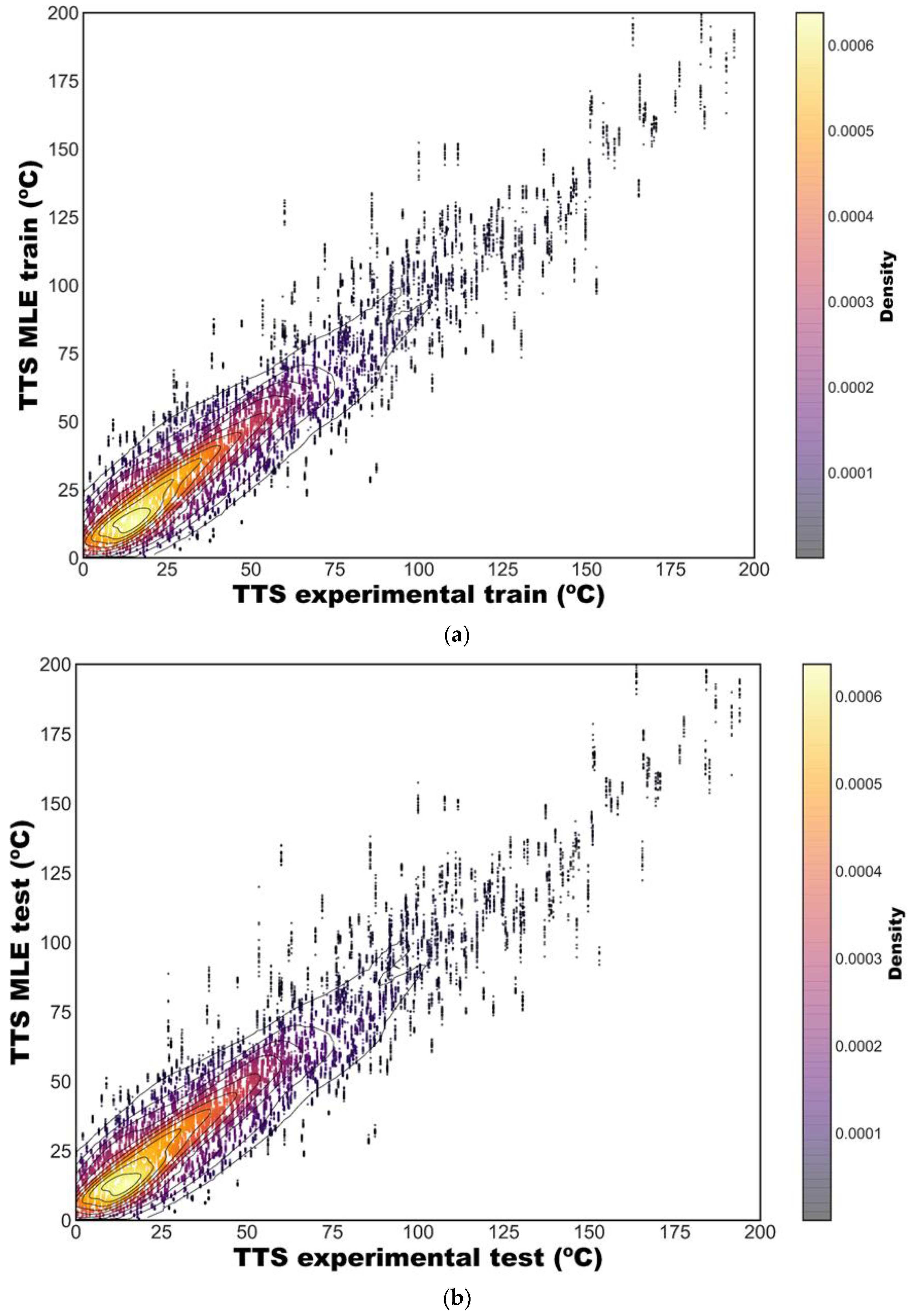
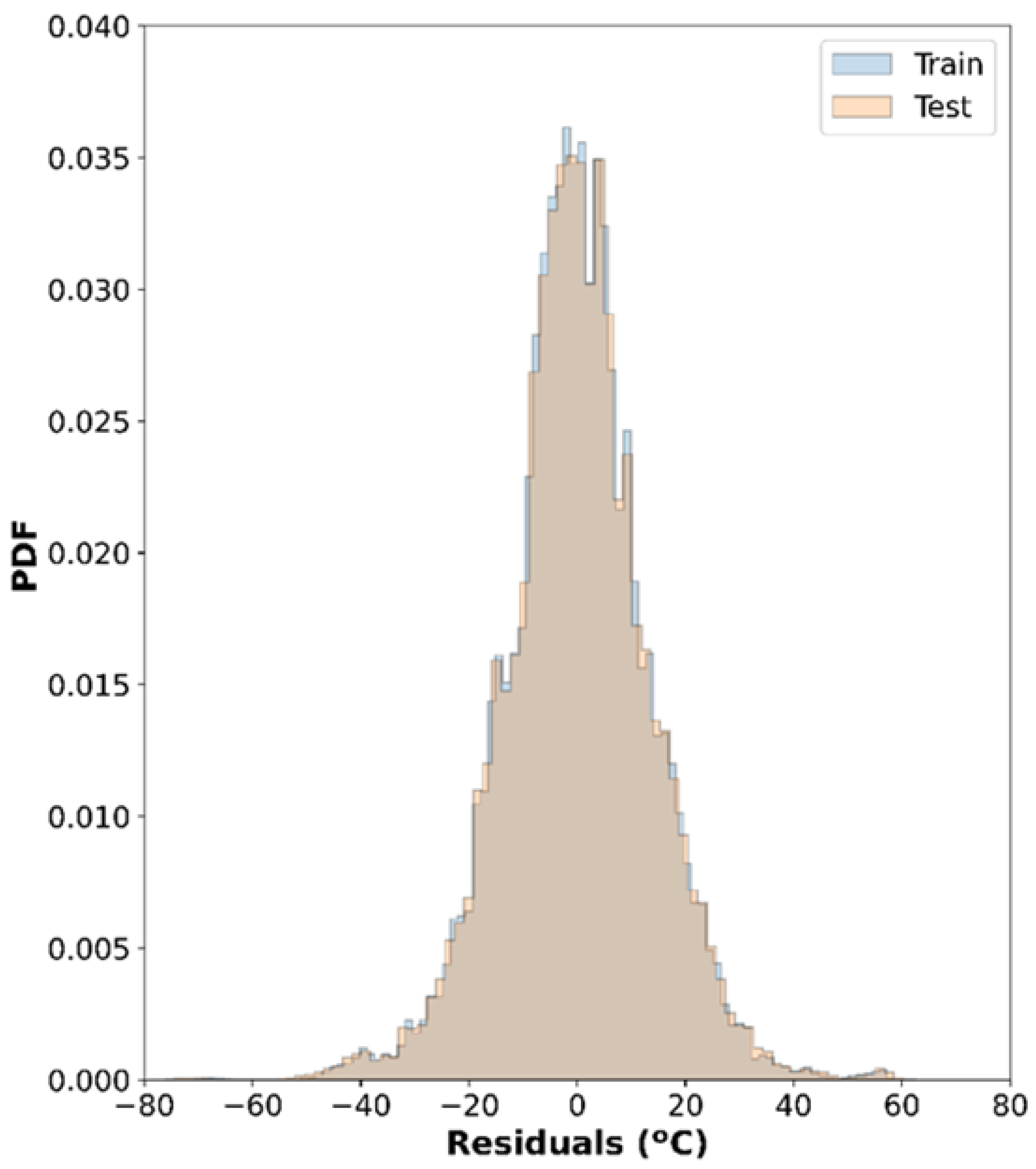
Some figures have been composed to visually appreciate the possible differences between the prediction capacity of the model on the train and test sets. In Figure 2, two scatterplots can be seen where the experimental TTS is compared with the value obtained through MLE for the train (a) and test (b) sets; the data are represented as a color map based on the density of points, and iso-density contour lines have been superimposed. Similarly, Figure 3 shows the distributions of residuals obtained in the train and test sets. However, none of these figures enables identification of differences between both sets that could be associated with overfitting: Figure 2b are indistinguishable in practice and the distributions of residuals in Figure 3 are virtually overlapping.

3.2. Inferential Statistics

Hypothesis tests were employed to detect statistically significant differences in the mean and variance between the train and test groups. The two-sample t-test was selected to compare the means of these two groups. This is a parametric method that assumes that data are independent, approximately normally distributed, and have similar variance within each group (homogeneity of variance). The condition of independence was guaranteed through the random splitting carried out as a part of the MCCV. The t-test assumes that the means of the different samples (not the samples themselves) are normally distributed; by virtue of the central limit theorem, means of samples from a population with finite variance approach a normal distribution, regardless of the distribution of the population. As a rule of thumb, sample means are normally distributed, provided that the sample size is at least 30 [20]. The equal variance condition was assessed through the Levene test, obtaining a p-value (which represents the probability of obtaining a test results at least as extreme as the results actually observed, under the assumption that the null hypothesis is correct), p ≈ 0, which enables rejecting the null hypothesis of equal variances (see Table 2, where the RMSEs obtained for the train and test sets are included). If variances are unequal, the library scipy [13] performs the Welch’s t-test [21], rather than the conventional Student’s t-test, because it does not assume equal population variance. In this case, the p-value was p = 9.581 × 10⁻³, which enables rejecting the null hypothesis of equal means at the 0.05 significance level. According to these results, there is a robust statistical evidence to reject both the hypothesis of means equality and variances equality of the sampling distributions of the residuals in the train and test sets. This outcome, which is in apparent contradiction with the visual inspection of Figure 2 and Figure 3, is explained in Section 4.

3.3. Assessment of Parameters

As an additional result derived from this research, the 5000 iterations of MCCV enable obtaining not only a point estimate for the 26 parameters of the ASTM E900-15 [3] ETC, but also the distribution of each one of them and, therefore, their confidence intervals. In this way, it is possible to assess the adequacy of the specific numerical values present in the ASTM E900-15 [3] standard and to consider possible improvements. From the distribution of parameters obtained through MCCV, some selected statistics (mean, standard deviation (SD)) and several quantiles (2.5%, 25%, 50%, 75%, and 97.5%) have been obtained for each of them, as can be seen in

Table 3. Relevant statistics of the distributions of the parameters of the ASTM E900-15 [3] ETC. These values were calculated from the distributions obtained by means of the MCCV method.

	Mean	SD	2.5%	25%	50%	75%	97.5%
CuMAX	2.765 × 10−1	1.071 × 10−2	2.532 × 10−1	2.734 × 10−1	2.772 × 10−1	2.836 × 10−1	2.921 × 10−1
CuMIN	5.415 × 10−2	2.193 × 10−3	4.880 × 10−2	5.299 × 10−2	5.418 × 10−2	5.539 × 10−2	5.765 × 10−2
M_Weld	9.740 × 10−1	1.579 × 10−1	6.515 × 10−1	8.781 × 10−1	9.747 × 10−1	1.071	1.290
M_Plate	7.924 × 10−1	1.276 × 10−1	5.305 × 10−1	7.153 × 10−1	7.939 × 10−1	8.708 × 10−1	1.046
M_Forge	7.462 × 10−1	1.258 × 10−1	4.938 × 10−1	6.686 × 10−1	7.465 × 10−1	8.242 × 10−1	9.983 × 10−1
M_slope	1.156 × 102	18.70	78.57	1.042 × 102	1.152 × 102	1.267 × 102	1.546 × 102
M_Maxslope	6.274 × 102	1.000 × 102	4.290 × 102	5.663 × 102	6.251 × 102	6.837 × 102	8.304 × 102
M_lnMinFlu	4.212 × 1020	7.031 × 1019	2.983 × 1020	3.707 × 1020	4.109 × 1020	4.781 × 1020	5.503 × 1020
M_Texp	−4.968	6.024 × 10−1	−6.174	−5.355	−4.978	−4.575	−3.763
M_Pconst	−2.034 × 10−2	1.073 × 10−1	−1.250 × 10−1	−1.248 × 10−1	−3.974 × 10−2	5.518 × 10−2	2.107 × 10−1
M_Pexp	−1.669 × 10−1	4.227 × 10−2	−2.490 × 10−1	−1.942 × 10−1	−1.679 × 10−1	−1.408 × 10−1	−7.904 × 10−2
M_Niconst	−2.147 × 10−2	1.780 × 10−1	−4.188 × 10−1	−1.305 × 10−1	4.851 × 10−3	1.092 × 10−1	2.604 × 10−1
M_Niexp1	4.257 × 10−1	1.843 × 10−1	1.656 × 10−1	2.893 × 10−1	3.978 × 10−1	5.239 × 10−1	8.665 × 10−1
M_Niexp2	1.013	3.740 × 10−1	4.613 × 10−1	7.530 × 10−1	9.436 × 10−1	1.210	1.909
B_Weld	7.754 × 10−1	1.697 × 10−1	4.266 × 10−1	6.638 × 10−1	7.880 × 10−1	8.903 × 10−1	1.089
B_Plate	9.141 × 10−1	2.009 × 10−1	5.046 × 10−1	7.841 × 10−1	9.308 × 10−1	1.049	1.283
B_Forge	8.479 × 10−1	1.864 × 10−1	4.650 × 10−1	7.270 × 10−1	8.611 × 10−1	9.763 × 10−1	1.185
B_Const	1.360 × 10−12	4.274 × 10−13	6.130 × 10−13	1.019 × 10−12	1.362 × 10−12	1.678 × 10−12	2.167 × 10−12
B_Exp	5.725 × 10−1	5.673 × 10−3	5.634 × 10−1	5.687 × 10−1	5.715 × 10−1	5.758 × 10−1	5.859 × 10−1
B_Texp	−5.787	4.408 × 10−1	−6.715	−6.062	−5.782	−5.494	−4.938
B_Pconst	1.891 × 10−1	1.092 × 10−1	3.516 × 10−2	1.161 × 10−1	1.686 × 10−1	2.392 × 10−1	4.596 × 10−1
B_Pexp	2.957 × 10−1	6.033 × 10−2	1.957 × 10−1	2.557 × 10−1	2.890 × 10−1	3.279 × 10−1	4.343 × 10−1
B_Niconst	4.075	1.385	1.943	3.073	3.866	4.878	7.294
B_Niexp1	9.727	1.912	6.752	8.415	9.476	10.71	14.28
B_Niexp2	4.452 × 10−1	1.022 × 10−1	0.2749	0.3770	0.4327	0.5009	0.6821
B_Mnexp	2.191 × 10−1	6.646 × 10−2	9.460 × 10−2	1.743 × 10−1	2.185 × 10−1	2.621 × 10−1	3.562 × 10−1

(the labels of the parameters shown in Table 3 were introduced for Table 1; see Section 2.1). Comparing Table 3 with Table 1, it can be seen that all but one of the parameters of ASTM E900-15 [3], B_Niconst, belong to the 95% confidence interval provided by the MCCV procedure.

To provide a more detailed description, Figure 4 shows the histogram obtained by means of MCCV for each of the 26 parameters. The red dotted line superimposed on each figure corresponds to the actual value in ASTM E900-15 [3]. In the majority of cases, the distributions exhibit a smooth unimodal histogram and the red dotted lines are close to the mode. In some parameters (CuMAX, CuMIN, M_lnMinFlu), bimodal distributions can be seen. This reflects the existence of close local maxima in the likelihood hyperspace. One of the advantages of the MCCV method implemented in this study is precisely the possibility of examining the distributions of the parameters, something that is not available if a conventional point estimate is carried out, as in ASTM E900-15.

In order to assess the margin for improvement derived from the MCCV method used in this research, the parameters of the ASTM E900-15 [3] ETC (collected in Table 1) have been replaced, respectively, by the mean and median values of the distributions shown in Figure 4 (the results of the MCCV analysis). Then, the TTS of the 1878 observations in the PLOTTER database have been re-estimated. In both cases, the results are basically the same, namely, RMSE = 13.24 °C and R² = 0.876 (there are no differences when the means or medians are used). Considering that the uncertainty scores of ASTM E900-15 [3] are RMSE = 13.32 °C and R² = 0.875, it can be concluded that the improvement of these parameters compared to the ones adopted in ASTM E900-15 is absolutely negligible.

4. Discussion

This paper describes the results obtained after applying the MCCV resampling technique on the samples of the PLOTTER database that were used to adjust the 26 parameters of the ASTM E900-15 [3] embrittlement trend curve that enables estimating the TTS experienced by nuclear vessel subjected to neutron irradiation as a function of their nature and exposure conditions. The hypotheses of our study were, on the one hand, that an analytical model as complex as the expression of the ASTM E900-15 [3] standard could be prone to overfitting and, on the other hand, that the parameters currently present in that expression would be susceptible to improvement using appropriate resampling techniques. An overfitted model of any type, either analytical or numerical, works very well with the sample data used to train its internal parameters but often provides disastrous results on new observations completely undermining the usefulness of the prediction model. The resampling technique used in this study is completely general since it can be used in any type of model to flag overfitting and to obtain confidence intervals of the fitted parameters.

After 5000 iterations of MCCV, large training and test datasets was generated containing 7,035,000 and 2,355,000 instances. The first can be considered as the control group of the experiment while the second plays the role of the treatment group. The statistical metrics used for the comparison of both groups exhibit subtle differences. Thus, in the training set, RMSE = 13.22 °C and R² = 0.877, while in the test set, RMSE = 13.53 °C and R² = 0.871. The distributions of residuals in both samples were compared using inferential statistics. Statistically significant differences at the 0.05 significance level were obtained between both the means (p = 9.581 × 10⁻³ in the Welch’s t-test) and the variances (p ≈ 0 in the Levene test). This strong statistical outcome contrasts with the subtle differences mentioned above regarding the predictive capacity in both sets. However, this result, which may seem paradoxical, can be properly interpreted from a correct understanding of the meaning of the p-value in statistics. In 2016, the American Statistical Association released a statement [22] warning against the misuse of statistical significance and p-values. As stated by Amrhein et al. [23], “bucketing results into ‘statistically significant’ and ‘statistically non-significant’ makes people think that the items assigned in that way are categorically different”, which is a mistake. Moreover, they recommend authors to describe the practical implications of all values inside the confidence interval. In our case, we detected statistically significant differences (at the customary 0.05 significance level) between the means and variances of the distributions of residuals in the train and test sets but, at the same time, reported, based on descriptive statistical considerations, that these differences are of minor magnitude and can be neglected on practical terms.

In addition, we used the results derived from the MCCV procedure to recalibrate the parameters of the ASTM E900-15 standard [3]; however, the improvement was negligible (RMSE = 13.24 °C and R² = 0.876 compared to the original scores, RMSE = 13.32 °C and R² = 0.875). The MCCV procedure made it possible to estimate the sampling distributions of the 26 parameters involved. In most cases, these follow a smooth, unimodal distribution but, in some cases, bimodal distributions suggesting the existence of close local maxima of the likelihood function have been observed. In general, these values deserve an individual analysis; however, the very slight differences in practical terms on the final result (less than 0.1 °C in the RMSE) indicate that their influence is negligible.

5. Conclusions

Based on the evidence reported in this study, we consider that the expression currently included in the ASTM E900-15 [3] standard can be expected to generalize well to new observations, provided they have the same characteristics as those of the training set [6]. Moreover, its parameters can hardly be improved in practical terms. These results demonstrate that E900-15 is not overfit relative to the multi-national data set defined by the ASTM “PLOTTER” database and compel us, therefore, to reject our initial hypotheses and turn our research into a negative study. Nonetheless, we believe that negative results may also be important, provided they contribute to our knowledge of the topic. Several compelling arguments are given in a recent editorial in Nature [24] in favor of publishing negative results. In this specific case, the outcome of our study deserves consideration since, to the best of the authors’ knowledge, no previous study had addressed the issue of the possible overfitting of the ASTM E900-15 [3] embrittlement trend curve and this could have motivated wrong and potentially dangerous decisions in the assessment of the structural integrity of nuclear vessels. In addition, it is always desirable in statistical terms to obtain confidence intervals rather than a point estimate of a parameter. We also believe that the methods introduced in this paper should be implemented for future improvements in the current prediction model provided by ASTM.

References

1. USNRC. Regulatory Guide 1.99 (Revision 2): Radiation Embrittlement of Reactor Vessel Materials; USNRC: Washington, DC, USA, 1998.
2. Eason, E.D.; Odette, G.R.; Nanstad, R.K.; Yamamoto, T. A Physically Based Correlation of Irradiation-Induced Transition Temperature Shifts for RPV Steels; Oak Ridge National Laboratory: Oak Ridge, TN, USA, 2007.
3. ASTM E900-15e2; Standard Guide for Predicting Radiation-Induced Transition Temperature Shift in Reactor Vessel Materials. ASTM International: West Conshohocken, PA, USA, 2015.
4. Hashimoto, Y.; Nomoto, A.; Kirk, M.; Nishida, K. Development of new embrittlement trend curve based on Japanese surveillance and atom probe tomography data. J. Nucl. Mater. 2021, 553, 153007. [Google Scholar] [CrossRef]
5. Ferreño, D.; Serrano, M.; Kirk, M.; Sainz-aja, J.A. Prediction of the Transition-Temperature Shift Using Machine Learning Algorithms and the Plotter Database. Metals 2022, 12, 186. [Google Scholar] [CrossRef]
6. Guido, S.; Müller, A. Introduction to Machine Learning with Python. A Guide for Data Scientists; O’Reilly Media, Inc.: Newton, MA, USA, 2016; ISBN 978-1449369415. [Google Scholar]
7. Geron, A. Hands-On Machine Learning with Scikit-Learn and TensorFlow; O’Reilly Media, Inc.: Newton, MA, USA, 2017; ISBN 978-1491962299. [Google Scholar]
8. Chollet, F. Deep Learning with Python; Manning Publications: New York, NY, USA, 2018; ISBN 978-1617294433. [Google Scholar]
9. Adjunct for ASTM E900-15; Technical Basis for the Equation used to Predict Radiation-Induced Transition Temperature Shift in Reactor Vessel Materials. ASTM: West Conshohocken, PA, USA, 2015.
10. The 2018 Top Programming Languages-IEEE Spectrum. Available online: https://spectrum.ieee.org/the-2018-top-programming-languages (accessed on 30 December 2021).
11. Stack Overflow Developer Survey. 2019. Available online: https://insights.stackoverflow.com/survey/2019/ (accessed on 30 December 2021).
12. Montgomery, D.C.; Runger, G.C. Applied Statistics and Probability for Engineers; Wiley: Hoboken, NJ, USA, 1994; Volume 19, ISBN 0471204544. [Google Scholar]
13. Virtanen, P.; Gommers, R.; Oliphant, T.E.; Haberland, M.; Reddy, T.; Cournapeau, D.; Burovski, E.; Peterson, P.; Weckesser, W.; Bright, J.; et al. SciPy 1.0: Fundamental algorithms for scientific computing in Python. Nat. Methods 2020, 17, 261–272. [Google Scholar] [CrossRef] [PubMed] [Green Version]
14. Nelder, J.A.; Mead, R. A Simplex Method for Function Minimization. Comput. J. 1965, 7, 308–313. [Google Scholar] [CrossRef]
15. Wright, M. Direct search methods: Once scorned, now respectable. In Proceedings of the Numerical analysis: Proceedings of the 1995 Dundee Biennial Conference in Numerical Analysis; Griffiths, D., Watson, G., Eds.; Addison-Wesley: Boston, MA, USA, 1996; pp. 191–208. [Google Scholar]
16. Cawley, G.C.; Talbot, N.L.C. On over-fitting in model selection and subsequent selection bias in performance evaluation. J. Mach. Learn. Res. 2010, 11, 2079–2107. [Google Scholar]
17. Kuhn, M.; Johnson, K. Applied Predictive Modeling; Springer: New York, NY, USA, 2013; ISBN 978-1-4614-6848-6. [Google Scholar]
18. Dubitzky, W.; Granzow, M.; Berrar, D.P. (Eds.) Fundamentals of Data Mining in Genomics and Proteomics; Springer Science & Business Media: Berlin/Heidelberg, Germany, 2007; ISBN 978-0-387-47508-0. [Google Scholar]
19. Banerjee, A.V.; Duflo, E. Chapter 1—An Introduction to the “Handbook of Field Experiments.” In Handbook of Field Experiments; Banerjee, A.V., Duflo, E., Eds.; Elsevier: Amsterdam, The Netherlands, 2017; Volume 1, pp. 1–24. ISSN 2214-658X. [Google Scholar]
20. Lumley, T.; Diehr, P.; Emerson, S.; Chen, L. The importance of the normality assumption in large public health data sets. Annu. Rev. Public Health 2002, 23, 151–169. [Google Scholar] [CrossRef]
21. Welch’s t-test-Wikipedia. Available online: https://en.wikipedia.org/wiki/Welch%27s_t-test (accessed on 22 January 2022).
22. Wasserstein, R.L.; Lazar, N.A. The ASA’s Statement on p-Values: Context, Process, and Purpose. Am. Stat. 2016, 70, 129–133. [Google Scholar] [CrossRef] [Green Version]
23. Amrhein, V.; Greenland, S.; McShane, B. Retire statistical significance. Nature 2019, 567, 305–307. [Google Scholar] [CrossRef] [PubMed] [Green Version]
24. Mehta, D. Highlight negative results to improve science. Nature 2019. [Google Scholar] [CrossRef]
Figure 1. Flowchart describing the strategy followed in the study.
Metals 12 00481 g001
Figure 2. Scatterplots showing a comparison between experimental values of the TTS and the predictions obtained after fitting the free parameters by means of MLE using the data contained in the train set. Due to the impossibility of representing, respectively, 7,035,000 and 2,355,000 points in a figure, random subsets with 28,140 and 9420 observations, were represented. Notice that the proportions between sample sizes have been respected (28140/9420 = 7,035,000/2,355,000). (a) Train subset, (b) testing subset.
Metals 12 00481 g002
Figure 3. Distribution of residuals obtained in the train and tests subsets after MCCV. Both distributions contain 5000 observations.
Metals 12 00481 g003
Figure 4. Histograms showing the distributions (blue shaded region) of the ASTM E900-15 [3] parameters obtained in the train subset through MCCV. Each of these distributions contain 5000 observations. The figures also show the E900-15 point estimates (red vertical dotted line).
Metals 12 00481 g004