The Fundamental Formulation for Inhomogeneous Inclusion Problems with the Equivalent Eigenstrain Principle

Abstract

In this paper, and on the basis of the equivalent eigenstrain principle, a fundamental formulation for inhomogeneous inclusion problems is proposed, which is to transform the inhomogeneous inclusion problems into auxiliary equivalent homogenous inclusion problems. Then, the analysis, which is based on the equivalent homogenous inclusions, would significantly reduce the workload and would enable the analytical solutions that are possible for a series of inhomogeneous inclusion problems. It also provides a feasible way to evaluate the effective properties of composite materials in terms of their equivalent homogenous materials. This formulation allows for solving the problems: (i) With an arbitrarily connected and shaped inhomogeneous inclusion; (ii) Under an arbitrary internal load by means of the nonuniform eigenstrain distribution; and (iii) With any kind of external load, such as singularity, uniform far field, and so on. To demonstrate the implementation of the formulation, an oblate inclusion that interacts with a dilatational eigenstrain nucleus is analyzed, and an explicit solution is obtained. The fundamental formulation that is introduced here will find application in the mechanics of composites, inclusions, phase transformation, plasticity, fractures, etc.

1. Introduction

Inhomogeneous inclusion refers to a given arbitrarily shaped region (which is called an “inclusion”) in an infinite linear elastic space, and the region has elastic properties that are different from the surroundings (which are called the “matrix”). Of interest are the elastic fields inside and outside region that are generated by an arbitrarily prescribed eigenstrain that is distributed in the region, or by any kind of externally applied load. This problem is the so-called “inhomogeneous inclusion problem”. If the elastic properties of the inclusion are identical to the elastic properties of the matrix, it is called the “homogenous inclusion problem”. Because of their extremely broad applications in material science, such as in residual stress phenomena, phase transformation, reinforcing phases, material inhomogeneities, precipitates, defects, plastic strain or misfit strain, cracks, voids, etc., inclusion problems have been studied for more than one hundred years, ever since a pioneering result was published by Inglis [1], and, nowadays, inclusion mechanics is also regarded as one of the most attractive and challenging topics in solid mechanics (see, e.g., [2,3,4,5,6,7,8,9,10,11,12,13,14,15,16,17,18,19,20,21]). Numerous references have been devoted to this study, which can partly be found in the review papers by Mura and his coworkers [22,23], and by Zhou et al. [24], and in the books by Christensen [25], Mura [13], Nemat-Nasser and Hori [26], and Kachanov and Sevostianov [27].

A significant breakthrough is attributed to Eshelby [7,8], who generalized the earlier episodic results that pertain to ellipsoidal/elliptical inhomogeneities by proving the uniform nature of the internal strain field in all such inhomogeneities when the inclusion eigenstrain is uniform. This interesting result was elegantly formulated in terms of the classical fourth-order Eshelby tensor, which laid the foundation for a systematic exploration of the problems regarding inclusions in elastic solids (see, e.g., [11,28]). This model, as well as its related variations, has become one of the classical achievements in solid mechanics, and it has inspired great efforts to tackle a more generalized one, in which: (i) The inclusion can be of a nonellipsoidal shape; (ii) The eigenstrain in the inclusion can be nonuniform [9,29]; and (iii) The external load can be any kind of form.

Great efforts have been devoted to this generalized inhomogeneous problem, and significant progress has been made. The problem has been addressed in the general terms of the body force method, in which either the eigenstrain or the material difference between the matrix and the inhomogeneity can be fully incorporated as a fictitious body force (see, e.g., [30,31,32,33,34]). This theoretical contribution has often been used to estimate the effective elastic constants of composites (see, e.g., [27,32,35,36]).

Alternatively, following the basic idea of Eshelby’s equivalent inclusion method [13], we recently proposed the equivalent eigenstrain principle for inhomogeneous inclusion problems with nonellipsoidal shapes and nonuniform eigenstrain distributions [37]. The approach allows for directly transforming the inhomogeneous inclusion problem into an auxiliary equivalent homogeneous inclusion problem. The basic idea is to replace the inhomogeneous inclusion with an equivalent homogeneous one, which has a new equivalent eigenstrain distribution. Then, the homogenous inclusion can be easily solved by using Green’s function method (see, e.g., [13,38,39,40,41,42,43,44,45,46]). This treatment may largely simplify the difficulty of the original inhomogeneous inclusion problems, and, thus, the analytical solutions for a series of inhomogeneous inclusion problems with nonuniform eigenstrain distributions can be developed (see, e.g., [44,47,48,49]). Moreover, within the auxiliary equivalent homogenous inclusion problems, the effective elastic constants of composites, and the local stress field among the inhomogeneities, can be evaluated with less workload in comparison with the finite element method, which, therefore, can drastically reduce the computational cost (see, e.g., [50,51,52,53,54,55,56,57,58,59]). This is an evident advantage of the equivalent eigenstrain approach in comparison with the other methods for composite modeling.

In the aforementioned analysis, where the equivalent inclusion method is involved, the external load condition is mainly confined to a uniform far field. The arbitrary external load condition in inhomogeneous inclusion problems is actually a practical challenge, and it is comparable to the ones that only involve the nonuniform eigenstrain distribution. Sometimes, it can even turn out to be a more complex issue than the one with the prescribed internal eigenstrain distribution. On the other hand, there is the lack of a direct compact unified formulation in the equivalent eigenstrain approach, which should be versatile in order to model the arbitrarily connected and shaped inhomogeneous inclusion problems. In order to refine our previous work [37], and to broaden its application, a rigorous and unified formulation for generalized inhomogeneous inclusion problems needs to be performed. This is the basic motivation of this study.

The aim of this study is to complete and generalize the equivalent eigenstrain approach for formulating the inhomogeneity problems with nonellipsoidal shapes, nonuniform eigenstrain distributions, and that are subjected to arbitrary external loads. The present derivation follows the spirit of the equivalent eigenstrain principle that was proposed by the present authors before the publication of [37], but it expands its application to a broader range of the generalized inclusion problems.

The structure of the present report is as follows. In Section 2, the basic equations are presented. In Section 3, the fundamental formulation for solving the inhomogeneous inclusion problem is developed. In Section 4, a simple example of a flat inclusion interacting with a dilatational eigenstrain nucleus is presented in order to demonstrate its application. Subsequently, in Section 5, the numerical methods for solving the equivalent eigenstrain are discussed. In Section 6, the conclusions are drawn.

2. Fundamentals of Homogenous Inclusion Mechanics

In this section, the field equations for the elasticity theory, with particular reference to solving eigenstrain problems, are reviewed for the follow-up use. These include Hooke’s law of elasticity, equilibrium equations, and compatibility conditions, as well as the solution for homogenous inclusion problems.

2.1. Hooke’s Law and the Compatibility Condition

For infinitesimal deformations, the total strain (${\epsilon }_{ij}$) is regarded as the sum of the elastic strain ($e_{ij}$) and the eigenstrain (${\epsilon }_{ij}^{\ast }$):

$${\epsilon }_{ij}=e_{ij}+{\epsilon }_{ij}^{\ast }$$

(1)

The total strain (${\epsilon }_{ij}$) must be compatible, and it is expressed in terms of displacement ($u_i$) as:

$${\epsilon }_{ij}=\left(u_{i,j}+u_{j,i}\right)/2$$

(2)

The elastic strain is related to the stress (${\sigma }_{ij}$) by Hooke’s law:

$${\sigma }_{ij}=C_{ijkl}{e}_{kl}=C_{ijkl}\left({\epsilon }_{kl}-{\epsilon }_{kl}^{*}\right)=C_{ijkl}\left(u_{k,l}-{\epsilon }_{kl}^{*}\right)$$

(3)

where $C_{ijkl}$ are the elastic moduli, and the summation convention for the repeated indices is employed.

Since $C_{ijkl}=C_{ijlk}$, we have $C_{ijkl}{u}_{k,l}=C_{ijkl}{u}_{l,k}$. In the region where ${\epsilon }_{kl}^{*}=0$, Equation (3) becomes:

$${\sigma }_{ij}=C_{ijkl}{\epsilon }_{kl}=C_{ijkl}{u}_{k,l}$$

(4)

The inverse expression of (3) is:

$$\left({\epsilon }_{ij}-{\epsilon }_{ij}^{*}\right)=C_{ijkl}^{-1}{\sigma }_{kl}=S_{ijkl}{\sigma }_{kl}$$

(5)

where $C_{ijkl}^{-1}=S_{ijkl}$ is the elastic compliance.

2.2. Equilibrium Conditions

The equations of the equilibrium are:

$${\sigma }_{ij,j}+f_i=0, i=1,2,3$$

(6)

where $f_i$ is the body force. The boundary conditions for the external surface forces ($T_i$) are:

$$T_i={\sigma }_{ij}{n}_j$$

(7)

where $n_j$ is the exterior unit normal vector on the boundary of the body.

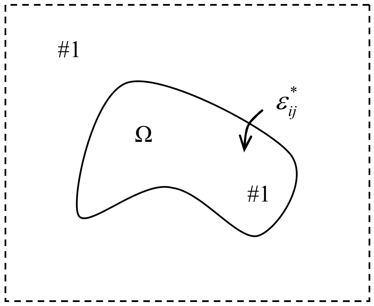
2.3. Solution for Homogenous Inclusion by Green’s Function Method

A homogeneous inclusion is embedded in an infinite solid (see Figure 1). If the profile of the inclusion is given, without going into details, then the deformation field can be easily obtained through the Green’s function method, as follows:

(a)

3-D inclusion [13]:

The displacement field in the inclusion will be:

$$u_i\left(x\right)=-{\displaystyle {\int }_{-\infty }^{\infty }{C}_{jlmn}{\epsilon }_{mn}^{*}\left(x^{\prime }\right)}{G}_{ij,l}\left(x-x^{\prime }\right)d{x}^{\prime }=-C_{jlmn}{\epsilon }_{mn}^{*}\left(x\right)\ast G_{ij,l}\left(x\right), x\in \mathsf{\Omega }$$

(8)

where the function, $G_{ij}\left(x-x^{\prime }\right)$, is the Green’s function, and is sometimes called the “influence function”. It has $G_{ij,l}\left(x-x^{\prime }\right)=\frac{\partial }{\partial x_l}{G}_{ij}\left(x-x^{\prime }\right)=-\frac{\partial }{\partial {x^{\prime }}_l}{G}_{ij}\left(x-x^{\prime }\right)$. The corresponding expressions for the strain and stress are as follows [13]:

$$\begin{array}{l}{\epsilon }_{ij}\left(x\right)=-\frac{1}{2}{\displaystyle {\int }_{-\infty }^{\infty }{C}_{klmn}{\epsilon }_{mn}^{*}\left(x^{\prime }\right)}\left\{G_{ik,lj}\left(x-x^{\prime }\right)+G_{jk,li}\left(x-x^{\prime }\right)\right\}d{x}^{\prime }\\ =-\frac{1}{2}{C}_{klmn}\left\{G_{ik,lj}\left(x\right)+G_{jk,li}\left(x\right)\right\}\ast {\epsilon }_{mn}^{*}\left(x\right)\\ =k_{ijmn}\left(x\right)\ast {\epsilon }_{mn}^{*}\left(x\right)\end{array}$$

(9)

and

$$\begin{array}{l}{\sigma }_{ij}\left(x\right)=C_{ijkl}{\displaystyle {\int }_{-\infty }^{\infty }{C}_{pqmn}\left\{G_{kp,qn}\left(x-x^{\prime }\right){\epsilon }_{ml}^{*}\left(x^{\prime }\right)-G_{kp,ql}\left(x-x^{\prime }\right){\epsilon }_{mn}^{*}\left(x^{\prime }\right)\right\}}d{x}^{\prime }\\ =C_{ijkl}{C}_{pqmn}\left\{G_{kp,qn}\left(x\right)\ast {\epsilon }_{ml}^{*}\left(x^{\prime }\right)-G_{kp,ql}\left(x\right)\ast {\epsilon }_{mn}^{*}\left(x\right)\right\}\end{array}$$

(10)

where

$$k_{ijmn}\left(x\right)=-\frac{1}{2}{C}_{klmn}\left\{G_{ik,lj}\left(x\right)+G_{jk,li}\left(x\right)\right\}=k_{ijnm}\left(x\right)=k_{jimn}\left(x\right)$$

(11)

where the operation symbol, ‘*’, stands for a convolution product. More details are listed in the “Appendix A”.

For isotropic materials:

$$C_{klmn}=\lambda {\delta }_{kl}{\delta }_{mn}+\mu \left({\delta }_{km}{\delta }_{ln}+{\delta }_{kn}{\delta }_{lm}\right)$$

(12)

The expression of the Green’s function for three-dimensional problems is:

$$G_{ij}\left(x\right)=\frac{1}{16\pi \mu \left(1-\nu \right)\left|x\right|}\left[\left(3-4\nu \right){\delta }_{ij}+\frac{x_i{x}_j}{{\left|x\right|}^2}\right]$$

(13)

where ${\delta }_{ij}$ is the Kronecker delta; ${\left|x\right|}^2=x_i{x}_i$; $\mu$ is the material’s shear modulus; and $\nu$ is the material’s Poisson ratio. Solution (13) was found by Lord Kelvin.

Equation (11) will be:

$$\begin{array}{l}{k}_{ijmn}\left(x\right)=-\frac{1}{2}{C}_{klmn}\left[G_{ik,lj}\left(x\right)+G_{jk,li}\left(x\right)\right]\\ =-\frac{1}{2}\left\{\lambda {\delta }_{mn}\left[G_{ik,kj}\left(x\right)+G_{jk,ki}\left(x\right)\right]+\mu \left[G_{im,nj}\left(x\right)+G_{in,mj}\left(x\right)+G_{jm,ni}\left(x\right)+G_{jn,mi}\left(x\right)\right]\right\}\end{array}$$

(14)

(b)

2-D inclusion:

Similarly, for isotropic materials, the expression of the Green’s function for two-dimensional problems can be written as [13]:

$$G_{ij}\left(x\right)=\frac{1}{2\pi \mu \left(1+\kappa \right)}\left[\frac{x_i{x}_j}{\left(x_1^2+x_2^2\right)}-\frac{\kappa {\delta }_{ij}}{2}\ln \left(x_1^2+x_2^2\right)\right]$$

(15)

where $\kappa =3-4\nu$ is the plane strain; and $\kappa =\left(3-\nu \right)/\left(1+\nu \right)$ is the plane stress.

Additionally, the complex potential Green’s function method is another convenient approach to treating two-dimensional problems [42,49].

In all, there is no significant difficulty in treating homogeneous inclusion problems, in theory.

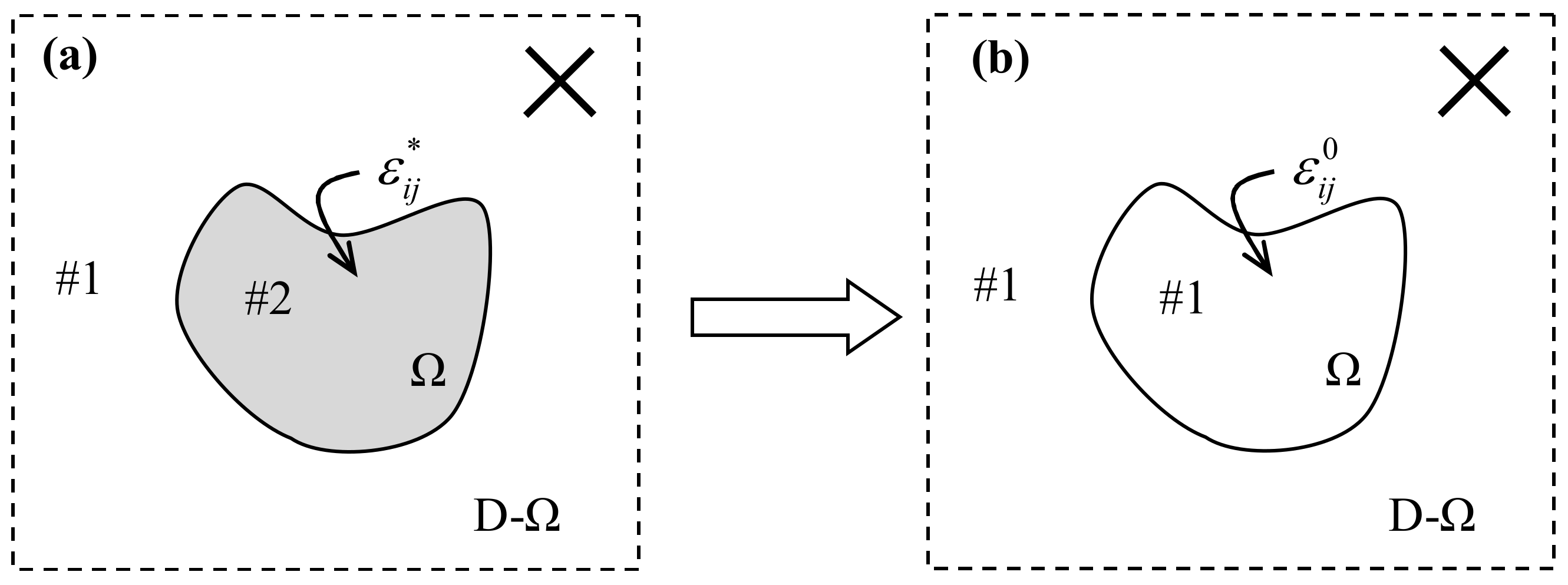
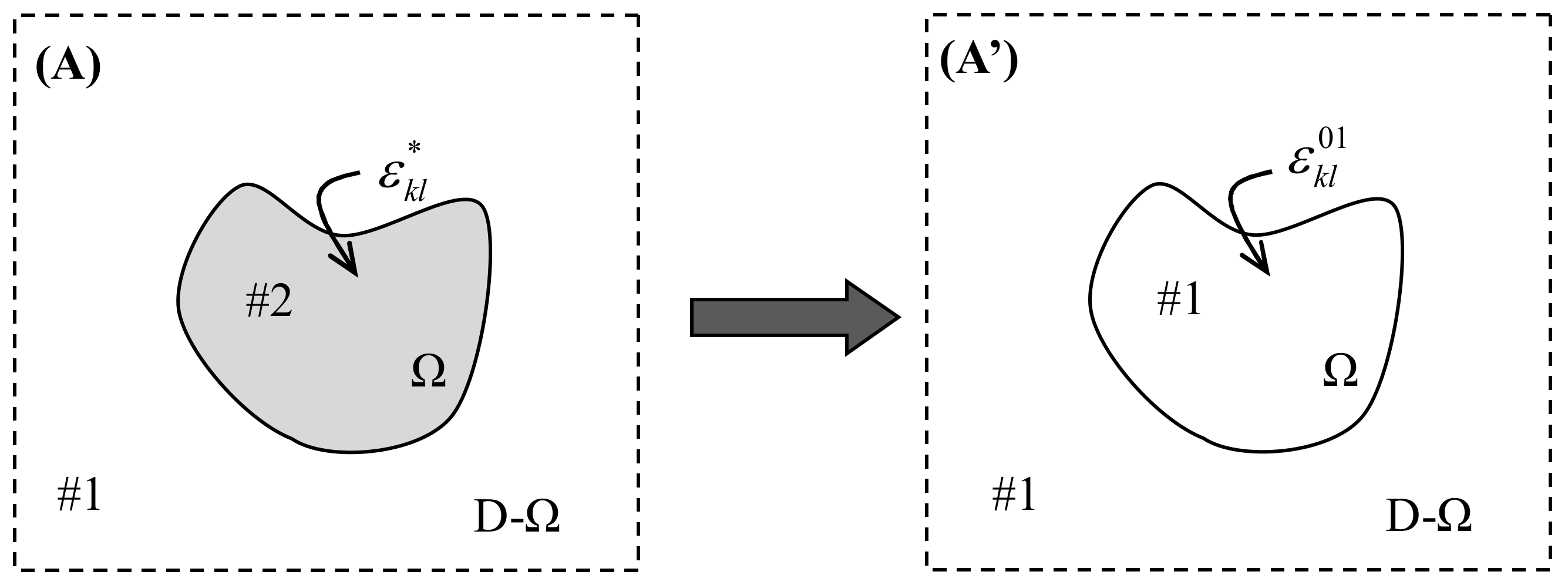
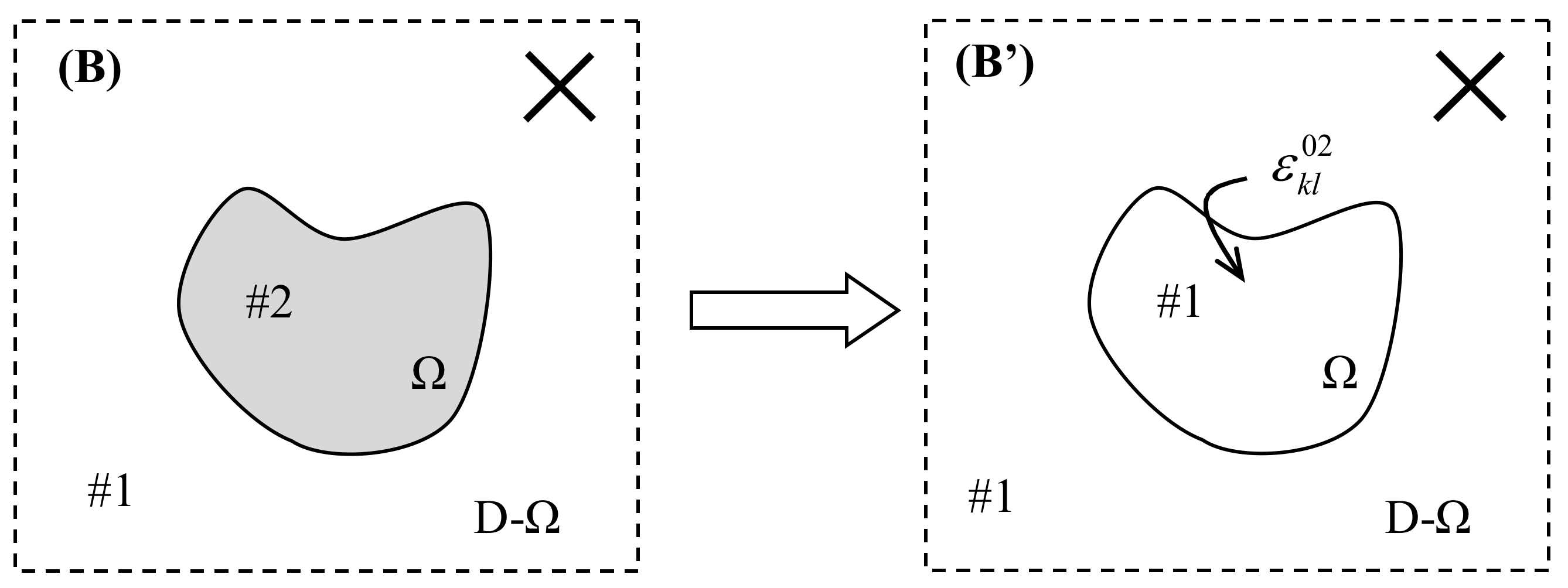
3. General Formulation for Inhomogeneous Inclusion Problems

Consider an arbitrarily shaped inhomogeneous inclusion that is embedded within an infinite solid. The inclusion is with a nonuniform eigenstrain distribution and is subjected to external loads, as is shown in Figure 2a, where the notation, X, may represent arbitrary loads, such as a concentrated force, a point-wise moment, a dislocation, a residual strain, a generalized singularity, a far-field load, or combinations, etc.

Theorem 1. 

An inhomogeneous inclusion, Ω, with an arbitrary shape and any inelastic strain distribution, embedded within a homogenous body, and subjected to arbitrary external loads, can be equaled by a homogeneous inclusion that accompanies an equivalent eigenstrain distribution within it. The stress and total strain distributions in the system do not change.

This can be put as:

$$C_{ijkl}^{*}\left({\epsilon }_{kl}+{\epsilon }_{kl}^X-{\epsilon }_{kl}^{*}\right)=C_{ijkl}\left({\epsilon }_{kl}+{\epsilon }_{kl}^X-{\epsilon }_{kl}^0\right), x\in \mathsf{\Omega }$$

(16)

where $C_{ijkl}^{*}$ and $C_{ijkl}$ are the elastic constants of the inclusion and the substrate, respectively; ${\epsilon }_{kl}^{*}$ is the given inelastic strain in the inhomogeneous inclusion; ${\epsilon }_{kl}^X$ is the elastic strain in the homogeneous inclusion that is induced by the known external load, which is denoted as, X; ${\epsilon }_{kl}^0$ is the equivalent eigenstrain in Figure 2b; and ${\epsilon }_{kl}$ is the total strain excited by ${\epsilon }_{kl}^0$, and it can be expressed in terms of the equivalent eigenstrain (${\epsilon }_{kl}^0$) as [13]:

$$\begin{array}{l}{\epsilon }_{ij}\left(x\right)=-\frac{1}{2}{\displaystyle {\int }_{-\infty }^{\infty }{C}_{klmn}{\epsilon }_{mn}^0\left(x^{\prime }\right)}\left\{G_{ik,lj}\left(x-x^{\prime }\right)+G_{jk,li}\left(x-x^{\prime }\right)\right\}d{x}^{\prime }\\ =-\frac{1}{2}{C}_{klmn}{\epsilon }_{mn}^0\left(x\right)\ast \left\{G_{ik,lj}\left(x\right)+G_{jk,li}\left(x\right)\right\}\\ =k_{ijmn}\left(x\right)\ast {\epsilon }_{mn}^0\left(x\right)\end{array}$$

(17)

Proof: 

According to the superposition principle, the original problem (Figure 2a) can be decomposed into two independent subproblems: Subproblem A and Subproblem B, as is shown in Figure 3. Subproblem A only has an inelastic strain load, while Subproblem B only has a generalized external load. □

Next, we will formulate the subproblems one by one.

Subproblem A:

According to the equivalent eigenstrain principle [37], the stress and total strain equalities in the two inclusion systems in Figure 4 result in:

$$C_{ijkl}^{*}\left({\epsilon }_{kl}^A-{\epsilon }_{kl}^{*}\right)=C_{ijkl}{e}_{kl}^{01}=C_{ijkl}\left({\epsilon }_{kl}^A-{\epsilon }_{kl}^{01}\right), x\in \mathsf{\Omega }$$

(18)

where the eigenstrain (${\epsilon }_{kl}^{*}$) is given; $e_{kl}^{01}$ and ${\epsilon }_{ij}^{01}$ are the elastic strain and the equivalent eigenstrain in (A′), respectively; and ${\epsilon }_{ij}^A$ is the total strain that is induced by ${\epsilon }_{ij}^{01}$, which can be expressed in terms of the equivalent eigenstrain (${\epsilon }_{ij}^{01}$) as:

$$\begin{array}{l}{\epsilon }_{ij}^A={\epsilon }_{ij}^{01}+e_{ij}^{01}=-\frac{1}{2}{\displaystyle {\int }_{-\infty }^{\infty }{C}_{klmn}{\epsilon }_{mn}^{01}\left(x^{\prime }\right)}\left\{G_{ik,lj}\left(x-x^{\prime }\right)+G_{jk,li}\left(x-x^{\prime }\right)\right\}d{x}^{\prime }\\ =-\frac{1}{2}{C}_{klmn}{\epsilon }_{mn}^{01}\left(x\right)\ast \left\{G_{ik,lj}\left(x\right)+G_{jk,li}\left(x\right)\right\}\\ =k_{ijmn}\left(x\right)\ast {\epsilon }_{mn}^{01}\left(x\right)\end{array}x\in \mathsf{\Omega }$$

(19)

Then, from Equations (18) and (19), we may obtain:

$$C_{ijkl}^{*}\left\{k_{klmn}\left(x\right)\ast {\epsilon }_{mn}^{01}\left(x\right)-{\epsilon }_{kl}^{*}\right\}=C_{ijkl}\left\{k_{klmn}\left(x\right)\ast {\epsilon }_{mn}^{01}\left(x\right)-{\epsilon }_{kl}^{01}\right\}, x\in \mathsf{\Omega }$$

(20)

From Equation (20), the sole unknown variable (${\epsilon }_{kl}^{01}$) can be fixed, which implies that Subproblem A is solved.

Subproblem B:

Again, according to the equivalent eigenstrain principle, the stress and total strain equalities in the two inclusion systems in Figure 5 lead to:

$$C_{ijkl}^{*}\left({\epsilon }_{kl}^B+{\epsilon }_{kl}^{\mathrm{X}}\right)=C_{ijkl}\left(e_{kl}^{02}+{\epsilon }_{kl}^{\mathrm{X}}\right)=C_{ijkl}\left({\epsilon }_{kl}^B+{\epsilon }_{kl}^{\mathrm{X}}-{\epsilon }_{kl}^{02}\right), x\in \mathsf{\Omega }$$

(21)

where ${\epsilon }_{kl}^{02}$ is the equivalent eigenstrain; $e_{kl}^{02}$ is the elastic strain that is induced by ${\epsilon }_{kl}^{02}$ in (B′); ${\epsilon }_{kl}^{\mathrm{X}}$ is the elastic strain that is induced by the generalized singularity, X, in (B′), which can be explicitly derived; and ${\epsilon }_{ij}^B$ is the strain that is related to ${\epsilon }_{kl}^{02}$ as:

$$\begin{array}{l}{\epsilon }_{ij}^B={\epsilon }_{ij}^{02}+e_{ij}^{02}=-\frac{1}{2}{\displaystyle {\int }_{-\infty }^{\infty }{C}_{klmn}{\epsilon }_{mn}^{02}\left(x^{\prime }\right)}\left\{G_{ik,lj}\left(x-x^{\prime }\right)+G_{jk,li}\left(x-x^{\prime }\right)\right\}d{x}^{\prime }\\ =-\frac{1}{2}{C}_{klmn}{\epsilon }_{mn}^{02}\left(x\right)\ast \left\{G_{ik,lj}\left(x\right)+G_{jk,li}\left(x\right)\right\}\\ =k_{ijmn}\left(x\right)\ast {\epsilon }_{mn}^{02}\left(x\right)\end{array},x\in \mathsf{\Omega }$$

(22)

so that Equation (21) can be written as:

$$C_{ijkl}^{*}\left\{k_{klmn}\left(x\right)\ast {\epsilon }_{mn}^{02}\left(x\right)+{\epsilon }_{kl}^{\mathrm{X}}\right\}=C_{ijkl}\left\{k_{klmn}\left(x\right)\ast {\epsilon }_{mn}^{02}\left(x\right)-{\epsilon }_{kl}^{02}+{\epsilon }_{kl}^{\mathrm{X}}\right\}, x\in \mathsf{\Omega }$$

(23)

It can be seen from Equation (23) that the sole unknown variable (${\epsilon }_{kl}^{02}$) can be fixed, which means that Subproblem B is solvable. It should be additionally explained that the total strain in Subproblem B is $\left({\epsilon }_{kl}^B+{\epsilon }_{kl}^{\mathrm{X}}\right)$ in Equation (21).

Thus, the equivalence between the original inhomogeneous model in Figure 2a and its counterpart auxiliary homogenous model in Figure 2b can be obtained by combining Equations (20) and (23) together as:

$$\begin{array}{l}{C}_{ijkl}^{*}\left\{k_{klmn}\left(x\right)\ast \left[{\epsilon }_{mn}^{01}\left(x\right)+{\epsilon }_{mn}^{02}\left(x\right)\right]+{\epsilon }_{kl}^{\mathrm{X}}-{\epsilon }_{kl}^{*}\right\}\\ =C_{ijkl}\left\{k_{klmn}\left(x\right)\ast \left[{\epsilon }_{mn}^{01}\left(x\right)+{\epsilon }_{mn}^{02}\left(x\right)\right]-\left[{\epsilon }_{kl}^{01}+{\epsilon }_{kl}^{02}\right]+{\epsilon }_{kl}^{\mathrm{X}}\right\}\end{array}, x\in \mathsf{\Omega }$$

(24)

This can be rewritten as:

$$C_{ijkl}^{*}\left\{\underset{¯}{k_{klmn}\left(x\right)\ast {\epsilon }_{mn}^0\left(x\right)+{\epsilon }_{kl}^X}-{\epsilon }_{kl}^{*}\right\}=C_{ijkl}\left\{\underset{¯}{k_{klmn}\left(x\right)\ast {\epsilon }_{mn}^0\left(x\right)+{\epsilon }_{kl}^X}-{\epsilon }_{kl}^0\right\}, x\in \mathsf{\Omega }$$

(25)

where

$${\epsilon }_{mn}^0\left(x\right)={\epsilon }_{mn}^{01}\left(x\right)+{\epsilon }_{mn}^{02}\left(x\right)$$

(26)

which is the only variable to be fixed in Equation (25). Equation (25) is the alternative formula of Equation (16). Up to now, the theorem has been proved.

Once ${\epsilon }_{mn}^0$ is solved from Equation (25), then the stress distribution in both the inclusion and the matrix can be calculated in the counterpart auxiliary homogeneous inclusion system as:

$${\sigma }_{ij}=\left\{\begin{array}{l}{C}_{ijkl}\left\{\left(k_{klmn}\ast {\epsilon }_{mn}^0\right)+{\epsilon }_{kl}^X-{\epsilon }_{kl}^0\right\},x\in \mathsf{\Omega }\\ C_{ijkl}\left\{\left(k_{klmn}\ast {\epsilon }_{mn}^0\right)+{\epsilon }_{kl}^X\right\} ,x\notin \mathsf{\Omega }\end{array}\right.$$

(27)

It should be explained that, in Equation (25), the sums with the underlines are the total strains, which are identical in the two systems. The results of both sides of Equation (25) are the stresses in both inclusions in Figure 2. Thus, the two inclusion systems that are shown in Figure 2 share identical total strain and stress distributions. This proof process is also the general formulation for inhomogeneous inclusion problems. Equation (25) transforms a generalized inhomogeneous inclusion into the corresponding easily solvable homogenous one. This equation is also called the “transform-governing equation” in this study.

In particular, it can be observed that Equation (16) or Equation (25) can be degenerated to the classical formula of the Eshelby solution (see pp. 178–189, [13]). In the original Eshelby inclusion model [6,7], the formulae, Equations (16) and (25), are held only if the inclusion system satisfies the Eshelby assumptions: (i) There is only one inclusion embedded within the infinite matrix; (ii) The inclusion is of an ellipsoidal shape; (iii) The eigenstrain in the inhomogeneous inclusion is uniform, and the remote load is also uniform. In comparison to the original Eshelby inclusion, Equation (16) or Equation (25) allow for calculating the elastic deformation of an arbitrarily connected and shaped inhomogeneous inclusion. The inelastic strain in inclusions can be nonuniform, and the external load can be any kind of force load, such as far-field loads, point-wise forces, moments, or displacement loads, such as dislocations, and so forth. It should be especially emphasized that when Equation (25) is applied to multi-inhomogeneity problems, the interaction among the inhomogeneities is automatically taken into account. The formula is suitable for both two-dimensional and three-dimensional inclusion problems.

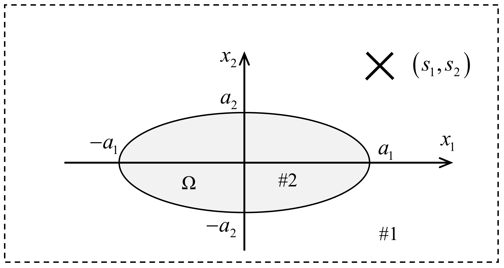
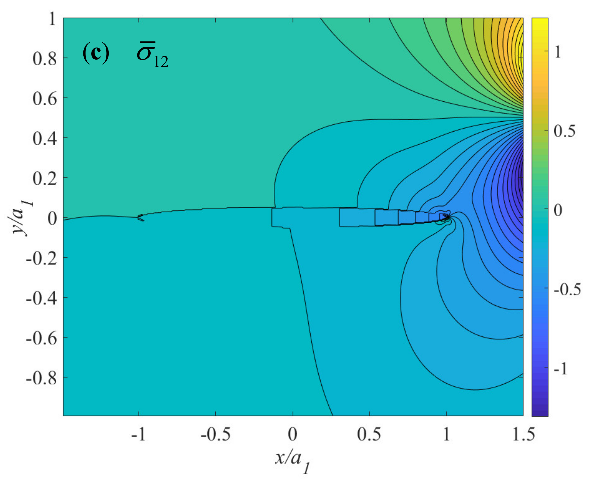
4. An Example: A Two-Dimensional Oblate Elliptical Inclusion Interacting with a Dilatational Eigenstrain Nucleus

To demonstrate the implementation of the formulation, we consider a two-dimensional problem where an oblate elliptical inclusion interacts with a dilatational eigenstrain nucleus, which is denoted with a cross notation, X, which is located at $\left(s_1,s_2\right)$, as is shown in Figure 6, where $a_2\ll a_1$, which is deliberately assumed to simplify the calculation in the following manipulations.

Assuming that the matrix and the inclusion materials are isotropic, the elastic constants degenerate as:

$$\left\{\begin{array}{l}{C}_{ijml}=\lambda {\delta }_{ij}{\delta }_{ml}+\mu \left({\delta }_{im}{\delta }_{jl}+{\delta }_{il}{\delta }_{jm}\right), \mathrm{for} \mathrm{matrix} \\ C^{*}{}_{ijml}={\lambda }^{\ast }{\delta }_{ij}{\delta }_{ml}+{\mu }^{\ast }\left({\delta }_{im}{\delta }_{jl}+{\delta }_{il}{\delta }_{jm}\right), \mathrm{for} \mathrm{inclusion}\end{array}\right.$$

(28)

in which $\lambda ,\mu ,{\lambda }^{\ast },{\mu }^{\ast }$ are the Lamé constants. The elastic strain, which is aroused by the dilatational eigenstrain nucleus in an infinite plane, can be obtained as [42,44]:

$$\begin{array}{l}{\epsilon }_{11}^X\left(x_1,x_2\right)=\frac{2\left[{\left(x_2-s_2\right)}^2-{\left(x_1-s_1\right)}^2\right]{\epsilon }_0}{\pi \left(1+\kappa \right){\left[{\left(x_1-s_1\right)}^2+{\left(x_2-s_2\right)}^2\right]}^2}\\ {\epsilon }_{22}^X\left(x_1,x_2\right)=\frac{2\left[{\left(x_1-s_1\right)}^2-{\left(x_2-s_2\right)}^2\right]{\epsilon }_0}{\pi \left(1+\kappa \right){\left[{\left(x_1-s_1\right)}^2+{\left(x_2-s_2\right)}^2\right]}^2}\\ {\epsilon }_{12}^X\left(x_1,x_2\right)=-\frac{4\left(x_1-s_1\right)\left(x_2-s_2\right){\epsilon }_0}{\pi \left(1+\kappa \right){\left[{\left(x_1-s_1\right)}^2+{\left(x_2-s_2\right)}^2\right]}^2}\end{array}$$

(29)

where $\left(s_1,s_2\right)$ are the coordinates of the singular point; ${\epsilon }_0$ is the strain nucleus intensity; and $\kappa =3-4\nu$ for the plane strain. Because $a_2\ll a_1$ in Figure 6, the elastic strain distribution within the homogenous inclusion that is due to the singularity can be approximated by letting $x_2=0$, as:

$$\begin{array}{l}{\epsilon }_{11}^X\left(x_1,0\right)=\frac{2\left[s_2{}^2-{\left(x_1-s_1\right)}^2\right]{\epsilon }_0}{\pi \left(1+\kappa \right){\left[{\left(x_1-s_1\right)}^2+s_2{}^2\right]}^2}\\ {\epsilon }_{22}^X\left(x_1,0\right)=\frac{2\left[{\left(x_1-s_1\right)}^2-s_2{}^2\right]{\epsilon }_0}{\pi \left(1+\kappa \right){\left[{\left(x_1-s_1\right)}^2+s_2{}^2\right]}^2}\\ {\epsilon }_{12}^X\left(x_1,0\right)=\frac{4\left(x_1-s_1\right)s_2{\epsilon }_0}{\pi \left(1+\kappa \right){\left[{\left(x_1-s_1\right)}^2+s_2{}^2\right]}^2}\end{array}, x_1\in \left(-a_1,a_1\right)$$

(30)

Thus, Equation (16) can be written as:

$$C^{*}\left(\epsilon +{\epsilon }^X\right)=C\left(\epsilon -{\epsilon }^0+{\epsilon }^X\right)$$

(31)

where

$$\begin{array}{l}{C}^{*}=\left[\begin{array}{ccc}{\lambda }^{\ast }+2{\mu }^{\ast }& {\lambda }^{\ast }& 0\\ {\lambda }^{\ast }& {\lambda }^{\ast }+2{\mu }^{\ast }& 0\\ 0& 0& 2{\mu }^{\ast }\end{array}\right],C=\left[\begin{array}{ccc}\lambda +2\mu & \lambda & 0\\ \lambda & \lambda +2\mu & 0\\ 0& 0& 2\mu \end{array}\right]\\ {\epsilon }^X=\left[\begin{array}{c}{\epsilon }_{11}^X\left(x_1,0\right)\\ {\epsilon }_{22}^X\left(x_1,0\right)\\ {\epsilon }_{12}^X\left(x_1,0\right)\end{array}\right],{\epsilon }^0=\left[\begin{array}{c}{\epsilon }_{11}^0\\ {\epsilon }_{22}^0\\ {\epsilon }_{12}^0\end{array}\right],\epsilon =\left[\begin{array}{c}{\epsilon }_{11}\\ {\epsilon }_{22}\\ {\epsilon }_{12}\end{array}\right]\end{array}$$

(32)

By virtue of Equation (9), the total strain can be expressed as:

$$\left[\begin{array}{c}{\epsilon }_{11}\\ {\epsilon }_{22}\\ {\epsilon }_{12}\end{array}\right]=\left[\begin{array}{ccc}{k}_{1111}\left(x\right)& k_{1122}\left(x\right)& 2k_{1112}\left(x\right)\\ k_{2211}\left(x\right)& k_{2222}\left(x\right)& 2k_{2212}\left(x\right)\\ k_{1211}\left(x\right)& k_{1222}\left(x\right)& 2k_{1212}\left(x\right)\end{array}\right]\ast \left[\begin{array}{c}{\epsilon }_{11}^0\left(x\right)\\ {\epsilon }_{22}^0\left(x\right)\\ {\epsilon }_{12}^0\left(x\right)\end{array}\right]$$

(33)

Without going into details, $k_{ijmn}$ in (33) can be specified by inserting (15) into (14): as

$$\begin{array}{l}{k}_{1111}\left(x\right)=-\frac{\left(3+\kappa \right)x_1{}^4-12x_1{}^2{x}_2{}^2+\left(1-\kappa \right)x_2{}^4}{2\pi \left(\kappa +1\right){\left(x_1^2+x_2^2\right)}^3},k_{1222}\left(x\right)=-\frac{4x_1{x}_2\left(3x_2{}^2-x_1{}^2\right)}{2\pi \left(1+\kappa \right){\left(x_1^2+x_2^2\right)}^3}\\ k_{1122}\left(x\right)=-\frac{\left(1-\kappa \right)x_1{}^4+12x_1{}^2{x}_2{}^2+\left(\kappa -5\right)x_2{}^4}{2\pi \left(\kappa +1\right){\left(x_1^2+x_2^2\right)}^3},k_{1211}\left(x\right)=-\frac{4x_1{x}_2\left(3x_1{}^2-x_2{}^2\right)}{2\pi \left(1+\kappa \right){\left(x_1^2+x_2^2\right)}^3}\\ k_{2211}\left(x\right)=-\frac{\left(\kappa -5\right)x_1{}^4+12x_1{}^2{x}_2{}^2+\left(1-\kappa \right)x_2{}^4}{2\pi \left(\kappa +1\right){\left(x_1^2+x_2^2\right)}^3},k_{1212}\left(x\right)=-\frac{2\left[6x_1{}^2{x}_2{}^2-x_2{}^4-x_1{}^4\right]}{2\pi \left(1+\kappa \right){\left(x_1^2+x_2^2\right)}^3}\\ k_{2222}\left(x\right)=-\frac{\left(1-\kappa \right)x_1{}^4-12x_1{}^2{x}_2{}^2+\left(3+\kappa \right)x_2{}^4}{2\pi \left(\kappa +1\right){\left(x_1^2+x_2^2\right)}^3}\\ k_{1112}\left(x\right)=-\frac{2x_1{x}_2\left[\left(\kappa -5\right)x_2{}^2+\left(\kappa +3\right)x_1{}^2\right]}{2\pi \left(1+\kappa \right){\left(x_1^2+x_2^2\right)}^3}\\ k_{2212}\left(x\right)=-\frac{2x_1{x}_2\left[\left(\kappa -5\right)x_1{}^2+\left(\kappa +3\right)x_2{}^2\right]}{2\pi \left(1+\kappa \right){\left(x_1^2+x_2^2\right)}^3}\end{array}$$

(34)

Because the minor axis ($a_2$) of the inclusion is much smaller than the major axis ($a_1$) in Figure 6, the inclusion can be treated as a very thin one, whose equivalent eigenstrain distribution can be reasonably approximated as: ${\epsilon }^0={\epsilon }^0\left(x_1\right)$. By skipping the derivation procedure, with this assumption (namely, $a_2\ll a_1$), and the following identities:

$$\underset{\Delta \to 0^{+}}{\lim }\frac{1}{\pi }\arctan \frac{\Delta }{x}=H\left(-x\right),\underset{\Delta \to 0}{\lim }\frac{2}{\pi }\frac{x^2\Delta }{{\left({\Delta }^2+x^2\right)}^2}=\delta \left(x\right),\underset{\Delta \to 0}{\lim }\frac{2}{\pi }\frac{{\Delta }^3}{{\left({\Delta }^2+x^2\right)}^2}=\delta \left(x\right)$$

(35)

the total strain in (33) can be simplified as:

$$\left[\begin{array}{c}{\epsilon }_{11}\\ {\epsilon }_{22}\\ {\epsilon }_{12}\end{array}\right]=\underset{a_2\to 0}{\lim }\left[\begin{array}{ccc}{k}_{1111}\left(x\right)& k_{1122}\left(x\right)& 2k_{1112}\left(x\right)\\ k_{2211}\left(x\right)& k_{2222}\left(x\right)& 2k_{2212}\left(x\right)\\ k_{1211}\left(x\right)& k_{1222}\left(x\right)& 2k_{1212}\left(x\right)\end{array}\right]\ast \left[\begin{array}{c}{\epsilon }_{11}^0\left(x\right)\\ {\epsilon }_{22}^0\left(x\right)\\ {\epsilon }_{12}^0\left(x\right)\end{array}\right]=\left[\begin{array}{ccc}-1& \frac{\left(\kappa -3\right)}{\left(\kappa +1\right)}& 0\\ -\frac{\left(\kappa -3\right)}{\left(\kappa +1\right)}& 1& 0\\ 0& 0& 0\end{array}\right]\left[\begin{array}{c}{\epsilon }_{11}^0\\ {\epsilon }_{22}^0\\ {\epsilon }_{12}^0\end{array}\right]=B{\epsilon }^0,x\in \mathsf{\Omega }$$

(36)

The matrix (B) is named as the “line inclusion tensor” [47]. This holds for any thin inclusion problems with uniform or nonuniform eigenstrain distributions.

Then, Equation (31) can be written as:

$$C^{*}\left(B{\epsilon }^0+{\epsilon }^X\right)=C\left(B{\epsilon }^0-{\epsilon }^0+{\epsilon }^X\right), x\in \mathsf{\Omega }$$

(37)

from which the equivalent eigenstrain is determined as:

$${\epsilon }^0={\left[C^{*}B-C\left(B-I\right)\right]}^{-1}\left(C-C^{*}\right){\epsilon }^X, x\in \mathsf{\Omega }$$

(38)

Thus, according to Equation (27), the stress distribution within the thin inclusion and the matrix will be:

$$\begin{array}{l}\sigma =C\left(B{\epsilon }^0-{\epsilon }^0+{\epsilon }^X\right)=C\left(B-I\right){\epsilon }^0+C{\epsilon }^X\\ =C\left(B-I\right){\left[C^{*}B-C\left(B-I\right)\right]}^{-1}\left(C-C^{*}\right){\epsilon }^X+C{\epsilon }^X\end{array}, x\in \mathsf{\Omega }$$

(39)

$$\left\{\begin{array}{l}{\sigma }_{11}=\lambda \left(k_{kkmn}\left(x\right)\ast {\epsilon }_{mn}^0\left(x\right)+{\epsilon }_{kk}^X\right)+2\mu \left(k_{11mn}\left(x\right)\ast {\epsilon }_{mn}^0\left(x\right)+{\epsilon }_{11}^X\right)\\ =\lambda \left[\left(k_{1111}+k_{2211}\right)\ast {\epsilon }_{11}^0+\left(k_{1122}+k_{2222}\right)\ast {\epsilon }_{22}^0+2\left(k_{1112}+k_{2212}\right)\ast {\epsilon }_{12}^0+{\epsilon }_{kk}^X\right]\\ +2\mu \left(k_{1111}\ast {\epsilon }_{11}^0+k_{1122}\ast {\epsilon }_{22}^0+2k_{1112}\ast {\epsilon }_{12}^0+{\epsilon }_{11}^X\right)\\ {\sigma }_{22}=\lambda \left(k_{kkmn}\left(x\right)\ast {\epsilon }_{mn}^0\left(x\right)+{\epsilon }_{kk}^X\right)+2\mu \left(k_{22mn}\left(x\right)\ast {\epsilon }_{mn}^0\left(x\right)+{\epsilon }_{22}^X\right)\\ =\lambda \left[\left(k_{1111}+k_{2211}\right)\ast {\epsilon }_{11}^0+\left(k_{1122}+k_{2222}\right)\ast {\epsilon }_{22}^0+2\left(k_{1112}+k_{2212}\right)\ast {\epsilon }_{12}^0+{\epsilon }_{kk}^X\right]\\ +2\mu \left(k_{2211}\ast {\epsilon }_{11}^0+k_{2222}\ast {\epsilon }_{22}^0+2k_{2212}\ast {\epsilon }_{12}^0+{\epsilon }_{22}^X\right)\\ {\sigma }_{12}=2\mu \left(k_{1211}\ast {\epsilon }_{11}^0+k_{1222}\ast {\epsilon }_{22}^0+2k_{1212}\ast {\epsilon }_{12}^0+{\epsilon }_{12}^X\right)\end{array}\right., x\notin \mathsf{\Omega }$$

(40)

where $k_{mnij}$ is given in (34); ${\epsilon }_{ij}^0\left(x_1\right)$ is given in (38); and the convolution, $k_{mnij}\ast {\epsilon }_{ij}^0$, can be expressed as:

$$\begin{array}{l}{k}_{mnij}\left(x_1,x_2\right)\ast {\epsilon }_{ij}^0\left(x_1\right)={\displaystyle {\int }_{-a_1}^{a_1}{\displaystyle {\int }_{-a_2\sqrt{1-{\left(\frac{{x^{\prime }}_1}{a_1}\right)}^2}}^{a_2\sqrt{1-{\left(\frac{{x^{\prime }}_1}{a_1}\right)}^2}}{k}_{mnij}\left(x_1-{x^{\prime }}_1,x_2-{x^{\prime }}_2\right){\epsilon }_{ij}^0\left({x^{\prime }}_1\right)d{x^{\prime }}_{2}d{x^{\prime }}_1}}\\ ={\displaystyle {\int }_{-a_1}^{a_1}{\displaystyle {\int }_{-a_2\sqrt{1-{\left(\frac{{x^{\prime }}_1}{a_1}\right)}^2}}^{a_2\sqrt{1-{\left(\frac{{x^{\prime }}_1}{a_1}\right)}^2}}{k}_{mnij}\left(x_1-{x^{\prime }}_1,x_2\right){\epsilon }_{ij}^0\left({x^{\prime }}_1\right)d{x^{\prime }}_{2}d{x^{\prime }}_1}}\\ =2a_2{\displaystyle {\int }_{-a_1}^{a_1}\sqrt{1-{\left(\frac{{x^{\prime }}_1}{a_1}\right)}^2}{k}_{mnij}\left(x_1-{x^{\prime }}_1,x_2\right){\epsilon }_{ij}^0\left({x^{\prime }}_1\right)d{x^{\prime }}_1}\end{array}$$

(41)

because $a_2\ll a_1$. Equations (39) and (40) are the general solutions for the problem in Figure 6.

It can be verified that the stress solutions, Equations (39) and (40), can be degenerated into a unified form when the materials of the inclusion and the matrix are identical. Alternately, if $C^{*}\to 0$, one finds that Equations (39) and (40) degenerate to the solution for a slit. This partially validates the preceding derivation.

To exhibit the interaction between the inclusion and the dilatational eigenstrain nucleus, the normalized stress (${\overline{\sigma }}_{ij}={\sigma }_{ij}\pi \left(\kappa +1\right)/8\mu {\epsilon }_0$) around the inclusion is numerically evaluated from Equations (39) and (40), and is plotted in Figure 7 for the case where ${\nu }^{\ast }/\nu =1$, ${\mu }^{\ast }/\mu =2$, $a_2/a_1=0.05$, and the singularity is located at $\left(s_1/a_1=2,s_2/a_1=0.5\right)$. It can be observed from Figure 7 that: (i) The stress distribution in both the matrix and the inclusion is nonuniformly distributed, and, because the inclusion is quite oblate, the stresses in the inclusion only vary with respect to x; (ii) The stress distribution is concentrated near the inclusion ends because of the sharp vertex of the inclusion and material inhomogeneity; and (iii) Since the inclusion is quite oblate (namely, $a_2\ll a_1$), the continuity of the stresses, ${\sigma }_{12}$ and ${\sigma }_{22}$, across the inclusion in a vertical direction remains roughly unchanged, while there is an evident jump in the stress (${\sigma }_{11}$) across the interface of the inclusion and the matrix. Such stress concentration and discontinuity phenomena imply that the initiation and the evolution of the damage potentially occur at these places when the inclusion system is subjected to complex load conditions.

It should be explained that the model in Figure 6 is very simple, but it is hardly to be treated directly within the framework of the original Eshelby inclusion mechanics. With the help of the equivalent eigenstrain principle, Equation (25) finally leads to the explicit solutions: Equations (39) and (40). For more complex problems, generally speaking, the numerical methods are inevitably employed to solve the equivalent eigenstrain from the transform governing Equation (25); then, the full stress field can be obtained. Thereafter, the detailed micromechanics analysis and the material design, such as the composites, can be legitimately performed.

5. Discussion of the Numerical Methods to Solve the Equivalent Eigenstrain

In terms of Equation (9):

$$k_{klmn}\left(x\right)\ast {\epsilon }_{mn}^0\left(x\right)={\displaystyle {\int }_{\mathsf{\Omega }}{k}_{klmn}\left(x-x^{\prime }\right){\epsilon }_{mn}^0\left(x^{\prime }\right)d{x}^{\prime }}, x\in \mathsf{\Omega }$$

(42)

and the transform governing Equation (25) can be rewritten as:

$$\left(C_{ijkl}^{*}-C_{ijkl}\right){\displaystyle {\int }_{\mathsf{\Omega }}{k}_{klmn}\left(x-x^{\prime }\right){\epsilon }_{mn}^0\left(x^{\prime }\right)d{x}^{\prime }}+C_{ijkl}{\epsilon }_{kl}^0=\left(C_{ijkl}-C_{ijkl}^{*}\right){\epsilon }_{kl}^X+C_{ijkl}^{*}{\epsilon }_{kl}^{*}, x\in \mathsf{\Omega }$$

(43)

The right side of Equation (43) is already given, and the only unknown variable is the equivalent eigenstrain: ${\epsilon }_{kl}^0$. This is an integral equation of the Lippmann–Schwinger type [32,60]. Once the equivalent eigenstrain (${\epsilon }_{kl}^0$) is fixed, the inclusion problem will be completely solved. A couple of related numerical methods have been developed in the literature, which can be directly adopted to numerically solve Equation (43). They are briefly introduced as follows:

(a)

The method of Taylor’s series expansion of the equivalent eigenstrain (see, e.g., [50,53,54,55,61]). The unknown equivalent eigenstrain in each inclusion can be expressed into a Taylor series with respect to the local origin of the inclusion, and the singular integrals will automatically become an integrable one [50]. The coefficients of the series are then determined by inserting them into the governing equation, Equation (43), which is also called the “consistency condition”;

(b)

The discretized element method. To find a more accurate numerical solution, the inhomogeneous inclusions are discretized into small elements, each of which is treated as a homogenous inclusion with an initial eigenstrain plus an unknown equivalent eigenstrain, according to the equivalent inclusion method (see, e.g., [56,58,59,62]), and the equivalent eigenstrain in each element should satisfy the discretized consistency condition Equation (43);

(c)

The Fourier transform method (or the numerical FFT method). The Fourier transform method has an evident advantage in treating the convolutions that are involved in Equation (43), and it may even lead to analytical solutions for some special problems [13], and for multi-inclusion problems [63]. With this in mind, a rough description for solving Equation (43) by Fourier transform is given below. It will lead to a general expression for the solution.

By performing the Fourier transform (see Appendix A) in Equation (43), we can obtain:

$$\left(C_{ijkl}^{*}{K}_{klmn}-C_{ijkl}{K}_{klmn}+C_{ijmn}\right)E_{mn}^0=\left(C_{ijkl}-C_{ijkl}^{*}\right)E_{kl}^X+C_{ijkl}^{*}{E}_{kl}^{*}$$

(44)

where

$$\begin{array}{l}{E}_{ml}^0\left(\xi \right)=\mathbb{F}\left[{\epsilon }_{ml}^0\right]=\frac{1}{{\left(2\pi \right)}^n}{\displaystyle {\int }_{{ℝ}^n}{\epsilon }_{ml}^0\left(x\right)e^{-ix\cdot \xi }dx}\\ E_{ml}^{*}\left(\xi \right)=\mathbb{F}\left[{\epsilon }_{ml}^{*}\right]=\frac{1}{{\left(2\pi \right)}^n}{\displaystyle {\int }_{{ℝ}^n}{\epsilon }_{ml}^{*}\left(x\right)e^{-ix\cdot \xi }dx}\\ E_{ml}^X\left(\xi \right)=\mathbb{F}\left[{\epsilon }_{ml}^X\right]=\frac{1}{{\left(2\pi \right)}^n}{\displaystyle {\int }_{{ℝ}^n}{\epsilon }_{ml}^X\left(x\right)e^{-ix\cdot \xi }dx}\\ K_{klmi}\left(\xi \right)=\mathbb{F}\left[k_{klmi}\right]=\frac{1}{{\left(2\pi \right)}^n}{\displaystyle {\int }_{{ℝ}^n}{k}_{klmi}\left(x\right)e^{-ix\cdot \xi }dx}\end{array}$$

(45)

The unknown variable ($E_{mn}^0$) can be determined from Equation (44), and then the equivalent eigenstrain would be solved through the inverse Fourier transform as:

$${\epsilon }_{ml}^0={\mathbb{F}}^{-1}\left[E_{ml}^0\right]={\displaystyle {\int }_{{ℝ}^n}{E}_{ml}^0\left(\xi \right)e^{ix\cdot \xi }d\xi }, x\in \mathsf{\Omega }$$

(46)

Thereafter, the stress field can be calculated within the equivalent homogenous inclusion as:

$${\sigma }_{ij}=\left\{\begin{array}{l}{C}_{ijkl}\left\{\left(k_{klmn}\ast {\epsilon }_{mn}^0\right)+{\epsilon }_{kl}^X-{\epsilon }_{kl}^0\right\},x\in \mathsf{\Omega }\\ C_{ijkl}\left\{\left(k_{klmn}\ast {\epsilon }_{mn}^0\right)+{\epsilon }_{kl}^X\right\} ,x\notin \mathsf{\Omega }\end{array}\right.$$

(47)

This is just a general solution expression of an elastic solution for inhomogeneous inclusion problems. As is seen by the use of the fast Fourier transform method (FFT) in the literature (see, e.g., [60,63,64,65]), it provides a more feasible approach for acquiring the numerical solution. Nevertheless, there is no doubt that it would take elaborate efforts to numerically treat different kinds of inhomogeneous inclusion problems in practice.

6. Conclusions

On the basis of the principle of the equivalent eigenstrain that is proposed, a fundamental formulation for solving inhomogeneous inclusion problems under arbitrary load conditions has been performed. This formulation allows for solving problems with arbitrarily shaped inclusions, any nonuniform eigenstrain distribution, as well as any kind of external load. It may lay a solid foundation for a systematic study of inhomogeneous inclusion problems in terms of the equivalent eigenstrain method. A simple example has been provided to demonstrate its implementation in solving inhomogeneous problems. It is expected that this formulation will be applied in the mechanics of composites, inclusions, phase transformation, plasticity, fractures, etc.

References

1. Inglis, C.E. Stresses in a plate due to the presence of cracks and sharp corners. Inst. Nav. Archit. Lond. 1913, 55, 219–230. [Google Scholar]
2. Mindlin, R.D. Force at a point in the interior of a semi-infinite solid. Physics 1936, 7, 195–202. [Google Scholar] [CrossRef]
3. Goodier, J.N. On the integration of the thermoelastic equations. Philos. Mag. 1937, 7, 1017–1032. [Google Scholar] [CrossRef]
4. Mindlin, R.D.; Cheng, D.H. Thermoelastic stress in the semi-infinite solid. J. Appl. Phys. 1950, 21, 931–933. [Google Scholar] [CrossRef]
5. Sen, B. Note on stresses produced by nuclei of thermo-elastic strain in a semi-infinite elastic solid. Q. Appl. Math. 1951, 8, 365–369. [Google Scholar] [CrossRef] [Green Version]
6. Hardiman, N.J. Elliptic elastic inclusion in an infinite elastic plate. Q. J. Mech. Appl. Math. 1954, 7, 226–230. [Google Scholar] [CrossRef]
7. Eshelby, J.D. The determination of the elastic field of an ellipsoidal inclusion, and related problems. Proc. R. Soc. Lond. A 1957, 241, 376–396. [Google Scholar]
8. Eshelby, J.D. The elastic field outside an ellipsoidal inclusion. Proc. R. Soc. Lond. A 1959, 252, 561–569. [Google Scholar]
9. Eshelby, J.D. Elastic inclusions and inhomogeneities. In Progress in Solid Mechanics; Sneddon, I.N., Hill, R., Eds.; North-Holland Publishing Company: Amsterdam, The Netherlands, 1961; Volume 2, pp. 89–140. [Google Scholar]
10. Jaswon, M.A.; Bhargava, R.D. Two-dimensional elastic inclusion problems. Proc. Camb. Philos. Soc. 1961, 57, 669–680. [Google Scholar] [CrossRef]
11. Mori, T.; Tanaka, K. Average stress in matrix and average elastic energy of materials with misfitting inclusions. Acta Metall. 1973, 21, 571–574. [Google Scholar] [CrossRef]
12. Willis, J.R. Variational and related methods for the overall properties of composites. Adv. Appl. Mech. 1981, 21, 1–78. [Google Scholar]
13. Mura, T. Micromechanics of Defects in Solids, 2nd ed.; Martinus Nijhoff: Dordrecht, The Netherlands, 1987. [Google Scholar]
14. Ru, C.Q. Analytical solution for Eshelby’s problem of an inclusion of arbitrary shape in a plane or half-plane. J. Appl. Mech. 1999, 66, 315–322. [Google Scholar] [CrossRef]
15. Ru, C.Q. Eshelby inclusion of arbitrary shape in an anisotropic plane or half plane. Acta Mech. 2003, 160, 219–234. [Google Scholar] [CrossRef]
16. Gong, S.X.; Meguid, S.A. On the elastic fields of an elliptical inhomogeneity under plane deformation. Proc. R. Soc. Lond. A 1993, 443, 457–471. [Google Scholar]
17. Zheng, Q.S.; Zhao, Z.H.; Du, D.X. Irreducible structure, symmetry and average of Eshelby’s tensor fields in isotropic elasticity. J. Mech. Phys. Solids 2006, 54, 368–383. [Google Scholar] [CrossRef]
18. Andrianov, I.V.; Argatov, I.I.; Weichert, D. On the absence of the Eshelby property for slender non-ellipsoidal inhomogeneities. Proc. R. Soc. A 2008, 464, 1079–1088. [Google Scholar] [CrossRef]
19. Zou, W.N.; He, Q.C.; Zheng, Q.S. General solution for Eshelby’s problem of 2D arbitrarily shaped piezoelectric inclusions. Int. J. Solids Struct. 2011, 48, 2681–2694. [Google Scholar] [CrossRef]
20. Chen, C.Q.; Cui, J.Z.; Duan, H.L.; Feng, X.Q.; He, L.H.; Hu, G.K.; Huang, M.J.; Huo, Y.Z.; Ji, B.H.; Liu, B.; et al. Perspectives in mechanics of heterogeneous solids. Acta Mech. Solida Sin. 2011, 24, 1–26. [Google Scholar] [CrossRef] [Green Version]
21. Chen, Q.D.; Xu, K.Y.; Pan, E. Inclusion of an arbitrary polygon with graded eigenstrain in an anisotropic piezoelectric half plane. Int. J. Solids Struct. 2014, 51, 53–62. [Google Scholar] [CrossRef] [Green Version]
22. Mura, T. Inclusion problems. Appl. Mech. Rev. 1988, 41, 15–20. [Google Scholar] [CrossRef]
23. Mura, T.; Shodja, H.M.; Hirose, Y. Inclusion problems. Appl. Mech. Rev. 1996, 49, S118–S127. [Google Scholar] [CrossRef]
24. Zhou, K.; Hoh, H.J.; Wang, X.; Keer, L.M.; Pang, J.H.L.; Song, B.; Wang, Q.J. A review of recent works on inclusions. Mech. Mater. 2013, 60, 144–158. [Google Scholar] [CrossRef]
25. Christensen, R.M. Mechanics of Composite Materials; Wiley: New York, NY, USA, 1979. [Google Scholar]
26. Nemat-Nasser, S.; Hori, M. Micromechanics: Overall Properties of Heterogeneous Materials, 2nd ed.; Elsevier: Amsterdam, The Netherlands, 1999. [Google Scholar]
27. Kachanov, M.; Sevostianov, I. Solid Mechanics and Its Applications; Springer Nature: Berlin/Heidelberg, Germany, 2018. [Google Scholar]
28. Hutchinson, J.W. Bounds and self-consistent estimates for creep of polycrystalline materials. Proc. R. Soc. Lond. A 1976, 348, 101–127. [Google Scholar]
29. Rahman, M. The isotropic ellipsoidal inclusion with a polynomial distribution of eigenstrain. J. Appl. Mech. 2002, 69, 593–601. [Google Scholar] [CrossRef]
30. Kunin, I.A.; Sosnina, E.G. An ellipsoidal inhomogeneity in an elastic medium. Proc. Acad. Sci. USSR 1971, 199, 571–575. [Google Scholar]
31. Kunin, I.A.; Sosnina, E.G. Stress concentration on an ellipsoidal inhomogeneity in an anisotropic elastic medium. Appl. Math. Mech. PMM 1973, 37, 306–315. [Google Scholar] [CrossRef]
32. Zeller, R.; Dederichs, P.H. Elastic Constants of Polycrystals. Phys. Status Solidi B 1973, 55, 831–842. [Google Scholar] [CrossRef]
33. Kunin, I.A. The Theory of Elastic Media with Microstructure II; Springer: Berlin/Heidelberg, Germany, 1983. [Google Scholar]
34. Kanaun, S.K.; Levin, V.M. Self-Consistent Methods for Composites Volume 1: Static Problems; Springer: Berlin/Heidelberg, Germany, 2008. [Google Scholar]
35. Kröner, E. Bounds for effective elastic moduli of disordered materials. J. Mech. Phys. Solids 1977, 25, 137–155. [Google Scholar] [CrossRef]
36. Willis, J.R. Bounds and self-consistent estimates for the overall properties of anisotropic composites. J. Mech. Phys. Solids 1977, 25, 185–202. [Google Scholar] [CrossRef]
37. Ma, L.F.; Korsunsky, A.M. The principle of equivalent eigenstrain for inhomogeneous inclusion problems. Int. J. Solids Struct. 2014, 51, 4477–4484. [Google Scholar] [CrossRef] [Green Version]
38. Johnson, W.C.; Earmme, Y.Y.; Lee, J.K. Approximation of the strain field associated with an inhomogeneous precipitate, Part 1. J. Appl. Mech. 1980, 47, 775–780. [Google Scholar] [CrossRef]
39. Johnson, W.C.; Earmme, Y.Y.; Lee, J.K. Approximation of the strain field associated with an inhomogeneous precipitate, Part 2. J. Appl. Mech. 1980, 47, 781–788. [Google Scholar] [CrossRef]
40. Li, Q.; Anderson, P.M. A compact solution for the stress field from a cuboidal region with a uniform transformation strain. J. Elast. 2001, 64, 237–245. [Google Scholar] [CrossRef]
41. Kuvshinov, B.N. Elastic and piezoelectric fields due to polyhedral inclusions. Int. J. Solids Struct. 2008, 45, 1352–1384. [Google Scholar] [CrossRef] [Green Version]
42. Ma, L.F. Fundamental formulation for transformation toughening. Int. J. Solids Struct. 2010, 47, 3214–3220. [Google Scholar] [CrossRef] [Green Version]
43. Avazmohammadi, R.; Hashemi, R.; Shodja, H.M.; Kargarnovin, M.H. Ellipsoidal domain with piecewise nonuniform eigenstrain field in one of joined isotropic half-spaces. J. Elast. 2010, 98, 117–140. [Google Scholar] [CrossRef]
44. Ma, L.F.; Wang, B.; Korsunsky, A.M. Plane deformation of circular inhomogeneous inclusion problems with non-uniform symmetrical dilatational eigenstrain. Mater. Des. 2015, 86, 809–817. [Google Scholar] [CrossRef]
45. Wang, X.; Chen, L.; Schiavone, P. Uniformity of stresses inside a non-elliptical inhomogeneity interacting with a mode III crack. Proc. R. Soc. Lond. A 2018, 474, 20180304. [Google Scholar] [CrossRef] [Green Version]
46. Dai, M.; Hua, J.; Schiavone, P. Compressible liquid/gas inclusion with high initial pressure in plane deformation: Modified boundary conditions and related analytical solutions. Eur. J. Mech. A Solid 2020, 82, 104000. [Google Scholar] [CrossRef]
47. Ma, L.F.; Qiu, Y.K.; Zhang, Y.M.; Li, G. General solution for inhomogeneous line inclusion with non-uniform eigenstrain. Arch. Appl. Mech. 2019, 89, 1723–1741. [Google Scholar] [CrossRef]
48. Wang, B.; Zhao, W.; Ma, L.F. Analysis of a finite matrix with an inhomogeneous circular inclusion subjected to a non-uniform eigenstrain. Arch. Appl. Mech. 2020, 90, 945956. [Google Scholar] [CrossRef]
49. Ma, L.F.; Tang, Z.Y.; Bian, Z.T.; Zhu, J.B.; Wiercigroch, M. Analytical solution for circular inhomogeneous inclusion problems with non-uniform axisymmetric eigenstrain distribution. Int. J. Mech. Sci. 2020, 194, 106213. [Google Scholar] [CrossRef]
50. Moschovidis, Z.A.; Mura, T. Two-ellipsoidal inhomogeneities by the equivalent inclusion method. J. Appl. Mech. 1975, 42, 847–852. [Google Scholar] [CrossRef]
51. Rodin, G.J.; Hwang, Y.L. On the problem of linear elasticity for an infinite region containing a finite number of non-intersecting spherical inhomogeneities. Int. J. Solids Struct. 1991, 27, 145–159. [Google Scholar] [CrossRef]
52. Fond, C.; Riccardi, A.; Schirrer, R.; Montheillet, F. Mechanical interaction between spherical inhomogeneities: An assessment of a method based on the equivalent inclusion. Eur. J. Mech. A/Solids 2001, 20, 59–75. [Google Scholar] [CrossRef]
53. Shodja, H.M.; Sarvestani, A.S. Elastic fields in double inhomogeneity by the equivalent inclusion method. J. Appl. Mech. 2001, 68, 3–10. [Google Scholar] [CrossRef]
54. Shodja, H.M.; Rad, I.Z.; Soheilifard, R. Interacting cracks and ellipsoidal inhomogeneities by the equivalent inclusion method. J. Mech. Phys. Solids 2003, 51, 945–960. [Google Scholar] [CrossRef]
55. Benedikt, B.; Lewis, M.; Rangaswamy, P. On elastic interactions between spherical inclusions by the equivalent inclusion method. Comput. Mater. Sci. 2006, 37, 380–392. [Google Scholar] [CrossRef]
56. Zhou, K.; Keer, L.M.; Wang, Q.J. Semi-analytic solution for multiple interacting three-dimensional inhomogeneous inclusions of arbitrary shape in an infinite space. Int. J. Numer. Methods Eng. 2011, 87, 617–638. [Google Scholar] [CrossRef]
57. Brisard, S.; Dormieux, L.; Sab, K. A variational form of the equivalent inclusion method for numerical homogenization. Int. J. Solids Struct. 2014, 51, 716–728. [Google Scholar] [CrossRef]
58. Zhou, Q.; Jin, X.; Wang, Z.; Wang, J.; Keer, L.M.; Wang, Q. Numerical Implementation of the Equivalent Inclusion Method for 2D Arbitrarily Shaped Inhomogeneities. J. Elast. 2015, 118, 39–61. [Google Scholar] [CrossRef]
59. Yang, W.; Zhou, Q.; Wang, J.; Khoo, B.C.; Phan-Thien, N. Equivalent inclusion method for arbitrary cavities or cracks in an elastic infinite/semi-infinite space. Int. J. Mech. Sci. 2021, 195, 106259. [Google Scholar] [CrossRef]
60. Moulinec, H.; Suquet, P. A numerical method for computing the overall response of nonlinear composites with complex microstructure. Comput. Methods Appl. Mech. Eng. 1998, 157, 69–94. [Google Scholar] [CrossRef]
61. Chen, F.C.; Young, K. Inclusions of arbitrary shape in an elastic medium. J. Math. Phys. 1977, 18, 1412–1416. [Google Scholar] [CrossRef]
62. Nakasone, Y.; Nishiyama, H.; Nojiri, T. Numerical equivalent inclusion method: A new computational method for analyzing stress fields in and around inclusions of various shapes. Mater. Sci. Eng. A 2000, 285, 229–238. [Google Scholar] [CrossRef]
63. Brisard, S.; Dormieux, L. Combining Galerkin approximation techniques with the principle of Hashin and Shtrikman to derive a new FFT-based numerical method for the homogenization of composites. Comput. Methods Appl. Mech. Eng. 2012, 217–220, 197–212. [Google Scholar] [CrossRef] [Green Version]
64. Moulinec, H.; Suquet, P. A fast numerical method for computing the linear and nonlinear properties of composites. Comptes Rendus Acad. Sci. Paris II 1994, 318, 1417–1423. [Google Scholar]
65. Eloh, K.S.; Jacquesa, A.; Berbenni, S. Development of a new consistent discrete green operator for FFT-based methods to solve heterogeneous problems with eigenstrains. Int. J. Plast. 2019, 116, 1–23. [Google Scholar] [CrossRef] [Green Version]
Figure 1. A homogeneous inclusion in an infinite elastic solid. (The material properties of the matrix and inclusion are identical, and they are denoted as material #1).
Metals 12 00582 g001
Figure 2. The equivalence of inhomogeneous inclusion and homogenous inclusion systems through the equivalent eigenstrain principle: (a) the original inhomogeneous inclusion system; (b) the counterpart auxiliary homogeneous inclusion system, in which #1 stands for the matrix material, and #2 stands for the inclusion, which occupies the domain (Ω). The cross, X, represents the external load.
Metals 12 00582 g002
Figure 3. Decomposition of the original problem in Figure 2a into two subproblems: (A) the system is solely under an internal load (inelastic strain distribution in the inhomogeneous inclusion); and (B) the system is solely under an external load, which is denoted with the notation, X, in which #1 stands for the matrix material, and #2 stands for the inclusion, which occupies the domain (Ω).
Metals 12 00582 g003
Figure 4. The equivalent eigenstrain principle: transformation from inhomogeneity to homogeneity, in which #1 stands for the matrix material, and #2 stands for the inclusion, which occupies the domain (Ω): (A) the original subproblem, A; (A′) the counterpart auxiliary homogeneous inclusion system of (A).
Metals 12 00582 g004
Figure 5. The equivalent eigenstrain principle: transformation from inhomogeneity to homogeneity, in which #1 stands for the matrix material, and #2 stands for the inclusion, which occupies the domain (Ω): (B) the original subproblem, B; (B′) the counterpart auxiliary homogeneous inclusion system of (B).
Metals 12 00582 g005
Figure 6. An oblate elliptical inclusion interacting with a dilatational eigenstrain nucleus, in which a 2 a 1 ; #1 stands for the matrix material; and #2 stands for the inclusion, which occupies the domain (Ω). In the system, the dilatational eigenstrain nucleus (the singularity) is denoted with a cross notation (X).
Metals 12 00582 g006
Figure 7. The normalized stress field of an oblate elliptical inclusion interacting with a dilatational eigenstrain nucleus, where ν / ν = 1 , μ / μ = 2 , a 2 / a 1 = 0.05 ; the singularity is located at s 1 / a 1 = 2 , s 2 / a 1 = 0.5 : (a) stress distribution of σ ¯ 11 = σ 11 π κ + 1 / 8 μ ε 0 ; (b) σ ¯ 22 = σ 22 π κ + 1 / 8 μ ε 0 , (c) σ ¯ 12 = σ 12 π κ + 1 / 8 μ ε 0 .
Metals 12 00582 g007aMetals 12 00582 g007b
Publisher’s Note: MDPI stays neutral with regard to jurisdictional claims in published maps and institutional affiliations.