Solidification Simulation of Al-Si Alloys with Dendrite Tip Undercooling

Abstract

A novel solution approach is proposed for the numerical simulation of the solidification process of binary Al-Si hypoeutectic alloys during upward and downward solidification modes. Undercooling is always observed during solidification, but the phenomenon could not be considered in the present-day numerical solution. In this approach, the temperature distribution in the mushy zone was used to define the fraction of solid, which enabled the evaluation of the effect of dendrite tip undercooling on the characteristics of the binary alloy solidification. The present numerical algorithm was found to significantly reduce the computation time. Transient temperature distribution and solidification time from the numerical analysis, with consideration of natural convection due to temperature and concentration gradients, have been successfully simulated and validated with experiment results. Numerical results with consideration of dendrite tip undercooling have better agreement with experimental results. The effect of dendrite tip undercooling on the fluid flow (velocity profile), G, R and λ₁ for both upward and downward solidification modes of Al-Si alloys have been investigated and discussed. Consideration of undercooling was found to increase G and reduce R in both solidification modes. During downward solidification, considering undercooling significantly increased flow velocity and decreased λ₁. The primary dendrite arm spacing could be validated with results from uni-directional solidification experiments only when dendrite tip undercooling was considered.

1. Nomenclature

cps	Specific heat of solid as a function of temperature (J Kg−1 K−1);
cpl	Specific heat of liquid (J Kg−1 K−1);
CL	Liquid concentration (wt%);
Co	Average alloy composition (wt%);
CS	Solid concentration (wt%);
D	Solute diffusivity coefficient of liquid (m2 s−1);
G	Temperature gradient in liquid at the mushy zone/liquid interface (°C mm−1);
K	Average partition coefficient;
Ks	Thermal conductivity of solid as a function of temperature (W m−1 K−1);
Kl	Thermal conductivity of liquid (W m−1 K−1);
L	Latent heat of fusion (J Kg−1);
M	The slope of liquidus line (K wt%−1);
P	Pressure (Pa);
R	Velocity of mushy zone/liquid interface (mm s−1);
t	Time (s);
T	Temperature (°C);
Tliq	Liquidus temperature (°C);
Tini	Initial temperature of liquid (°C);
Tm	Melting temperature of pure aluminum (°C);
Teut	Eutectic temperature (°C);
$\stackrel{.}{\mathrm{T}}$	Instantaneous tip cooling rate = G × R (°C s−1);
ΔT	Undercooling of Tliq (°C);
Ur	Velocity in r direction (mm.s−1);
uy	Velocity in y direction (mm.s−1);
U	Flow velocity in the liquid of mushy zone/liquid interface (mm.s−1);
β	Contraction ratio $\begin{array}{l}\left[\mathsf{\beta }=\frac{{\mathsf{\rho }}_{\mathrm{s}}-{\mathsf{\rho }}_{\mathrm{l}}}{{\mathsf{\rho }}_{\mathrm{l}}}\right]\\ \end{array}$ (volumetric shrinkage during solidification);
βC	Solute expansion coefficient (K−1);
βT	Thermal expansion coefficient (K−1);
Γ	Gibbs–Thomson coefficient (K m−1);
ϕ	Liquid fraction;
ρl	Liquid density (Kg m−3);
ρs	Solid density (Kg m−3);
µ	Dynamic viscosity (Pa s);
${\mathsf{\lambda }}_1^0$	Primary arm spacing if no fluid flow effect is considered (µm);
λ1	Primary arm spacing (µm)
Constant parameters
D	6.25 × 10−9 (m2 s−1) [1];
k	0.116 [2];
m	−6.675 (K wt%−1) [2];
Tm	(660 °C) [2];
Teut	(578.6 °C) [2];
Γ	1.97 × 10−7 (K m−1) [3];
βC	−4.26 × 10−4 (K−1) [4];
βT	1.39 × 10−4 (K−1) [4];
µ	1.3 × 10−3 (Pa s) [4];

2. Introduction

Solidification is the phenomenon of phase transformation from liquid phase to solid phase. Solidification mechanisms for pure metals and alloys are different from each other. Solidification for pure metals is mainly dominated by heat-transfer conditions [5,6]. However, both heat and mass transfer conditions affect the solidification of metallic alloys. During solidification of binary alloys, there are three distinct zones, namely, the liquid, solid and the intermediate two-phase (solid and liquid) region termed the mushy zone [7,8]. During the past few decades, there have been several attempts to simulate solidification of binary alloys [5,6,9,10,11,12,13,14]. These simulation attempts can be broadly classified into three categories:

• Solution to energy equation (thermal profiles) alone [14,15].
• Solution to both energy equation and concentration equation (solute concentration profiles) with the assumption of equilibrium solidification conditions; the liquid fraction ϕ in the two-phase mushy zone [8,9] would be evaluated using the Lever rule and/or Scheil–Gulliver equation [7].
• Solution to both energy and concentration equations (solute concentration profiles) with the assumption of equilibrium solidification condition and evaluate ϕ from the governing equations without lever rule or Scheil–Gulliver equation assumptions [10,12,16].

All the above-mentioned three categories of approaches could not circumvent the instability caused by the strong non-linearity arising from the phase transformation term in the energy equation. There has been a lack of validation of these models with experiments; validation of transient temperature distribution and time during solidification, because non-linearity from the phase transformation term impeded the successful solution of the coupled energy and concentration equations (to evaluate the transient liquid fraction in the two-phase mushy zone). Some of the common assumptions to circumvent the non-linearity include linearity in variation of temperature with ϕ [14,17] and absence of dendrite tip undercooling [7] of the dendrite tip temperature.

Undercooling at the dendrite tip can be caused by three factors: kinetics of solidification, rate of solute diffusion in the liquid and radius of the dendrite tip [7,18]. If the effect of dendrite tip undercooling was considered, the temperature and solute concentration gradients ahead of the dendrite tip would be higher because the temperature at the liquid/two-phase mushy zone interface would be lower than the T_liq [19]. Hence, assuming no undercooling will lead to erroneous evaluation of the dendrite arm spacing in the microstructure [20,21,22,23].

In solidification simulation of binary alloy, the dendrite tip undercooling could be included only if ϕ is determined directly from solving the energy equation. In the present work, a new approach to numerically simulate binary alloy solidification considering the effect of dendrite tip undercooling has been proposed wherein the energy equation alone is used to evaluate ϕ and a new coupling scheme for T and C_L inside the mushy zone has been utilized to avoid instability problems in the energy equation caused by the phase transformation term.

Presently, solidification simulations in the macro-scale (Control Volume, CV ~ 1 mm) do not predict the microstructural features of the solidified alloy such as primary and secondary dendrite arm spacings, λ₁ and λ₂, respectively [9,10,11,12,13,14]. One of the main reasons for this is the lack of accuracy in predicting the transient temperature distribution and hence, the progressive locations of the mushy zone/liquid interface (solidification time). The algorithm presented below enables predictions of λ₁ because the transient temperature distribution and the solidification times have been accurately predicted and validated with experiments: the reasons being that the new approach included the effect of dendrite tip undercooling prior to the solidification event, ΔT, and further optimized the materials properties as a function of temperature. Traditionally, the undercooling cannot be considered in solidification simulations of binary alloys because the order of magnitude of the diffusion coefficient of the solute in the liquid phase is four orders less than that of the thermal diffusivity and hence, the simulation with ΔT could not be practically completed. In this new approach, the liquid fraction ϕ in the mushy zone is evaluated by the energy equation with the heat transfer conditions that would enable successful completion of the simulation with the inclusion of the ΔT term. Evaluation of transient G and R would further enable prediction of λ₁, which would be a valuable tool to predict the solidification microstructure from a macro scale perspective. Further, the new simulation approach has been shown to be faster than the traditional counterpart [10,11,12].

3. Numerical Model

3.1. Background

Typically, during dendritic solidification in the mushy zone of a binary alloy, the interface temperature of the dendrite tip and the liquid will require an undercooling (ΔT) from the T_liq to sustain growth [7]. ΔT depends on G, R, Γ, k, D, m and C_o.

Burden et al. [24,25] presented an expression for ΔT as given in Equation (1). The magnitude of ΔT in Equation (1) was validated by experiments for cooling rates ranged up to 3 °C/s [24,25]. In this work, the magnitude of the dendrite tip undercooling is transient for the entirety of the solidification; it is updated after every time step for each control volume (CV).

$$\mathsf{\Delta }\mathrm{T}=\left(\frac{\mathrm{GD}}{\mathrm{R}}\right)+\frac{{\left(-8\mathrm{mR}\left(1-\mathrm{k}\right){\mathrm{C}}_{\mathrm{o}}\mathsf{\Gamma }\right)}^{\frac{1}{2}}}{{\mathrm{D}}_{}^{\frac{1}{2}}}$$

(1)

If numerical simulations do not consider ΔT, the estimation of G will be lower than the actual values in an experiment and this may lead to a prediction of shorter solidification times.

The early efforts to simulate binary alloy solidification by Voller et al. [14] considered only the energy equation (enthalpy balance) wherein the instability problem caused by strong non-linearity introduced by the phase transformation term was alleviated by assuming that the temperature in the mushy zone varied linearly with ϕ. The algorithm was not validated with any experiments. Subsequently, Bennon et al. [9] proposed a numerical algorithm to simulate alloy solidification using one form of the concentration and energy equations in all three zones (solid, liquid and mushy). The volume fraction of liquid was evaluated by applying equilibrium conditions (lever rule) and complete diffusion of solute in the solid was assumed, contrary to reality in a solidification experiment. Moreover, the ΔT value and the volumetric shrinkage (β) during phase transformation were also ignored. No experimental validation of the algorithm was presented.

A numerical algorithm for solidification simulation of binary alloys was proposed by Felicelli et al. [10]; wherein, the liquid fraction ϕ in the mushy zone was directly evaluated from the energy and concentration equations instead of the lever rule or Scheil–Gulliver paradigm [9]. One form of concentration equation was used to define the solute concentration in the solid, mushy zone and liquid regions alike. One form of energy equation was used in the solid and liquid regions. However, in the mushy zone, to alleviate the instability caused by the phase transformation term in the energy equation, the concentration equation substituted this term to obtain a modified form of the energy equation [9]; ϕ was evaluated from the concentration equation until the eutectic temperature was attained. Subsequently, at the eutectic temperature, ϕ has to be evaluated by the energy equation. ΔT was not used in this algorithm because concentration equation was used to determine ϕ in the bulk of the mushy zone and if ΔT was to be considered at the dendrite tip, then the completion of the solidification simulation would be practically impossible due to the very small order of D (~10⁻⁹ m.s⁻¹). An outline of the numerical algorithm used by Felicelli et al. [10] is shown in Figure 1. This algorithm has been one of the most popular methods this date to simulate binary alloy solidification [10,12]. This algorithm did not consider ΔT or β. However, McBride et al. [12] further developed this algorithm by considering β and the fluid flow occurring as a result of volumetric shrinkage. Heinrich et al. [11] corrected the flow fields during solidification at eutectic temperatures. No experimental validation in transient temperature distribution or solidification time of these numerical simulations has been carried out.

3.2. Governing Equations

Figure 2 presents schematic of the simulation conditions and the governing equations are presented herein: the energy equation is presented in Equation (2) and the concentration equation is Equation (3).

$$\begin{gathered} \stackrel{\mathrm{Transient} \mathrm{Term}}{\overbrace{\frac{\partial \left(\left({\mathsf{\phi }\mathsf{\rho }}_{\mathrm{l}}{\mathrm{c}}_{\mathrm{pl}}+\left(1-\mathsf{\phi }\right){\mathsf{\rho }}_{\mathrm{s}}{\mathrm{c}}_{\mathrm{ps}}\right)\mathrm{T}\right)}{\partial \mathrm{t}}}}+\stackrel{\mathrm{Convection} \mathrm{Term}}{\overbrace{{\mathsf{\rho }}_{\mathrm{l}}{\mathrm{c}}_{\mathrm{pl}}{\mathrm{u}}_{\mathrm{r}}\frac{\partial \mathrm{T}}{\partial \mathrm{r}}+{\mathsf{\rho }}_{\mathrm{l}}{\mathrm{c}}_{\mathrm{pl}}{\mathrm{u}}_{\mathrm{y}}\frac{\partial \mathrm{T}}{\partial \mathrm{y}}}}+\stackrel{\mathrm{Phase} \mathrm{Transformation} \mathrm{Term}}{\overbrace{{\mathsf{\rho }}_{\mathrm{s}}\mathrm{L}\frac{\partial \mathsf{\phi }}{\partial \mathrm{t}}}} \\ =\underset{\mathrm{Diffusion} \mathrm{Term}}{\underbrace{\frac{1}{\mathrm{r}}\frac{\partial }{\partial \mathrm{r}}(\mathrm{r}\left({\mathsf{\phi }\mathrm{K}}_{\mathrm{l}}+\left(1-\mathsf{\phi }\right){\mathrm{K}}_{\mathrm{s}}\right)\frac{\partial \mathrm{T}}{\partial \mathrm{r}})+\frac{\partial }{\partial \mathrm{y}}(({\mathsf{\phi }\mathrm{K}}_{\mathrm{l}}+\left(1-\mathsf{\phi }\right){\mathrm{K}}_{\mathrm{s}})\frac{\partial \mathrm{T}}{\partial \mathrm{y}})}} \end{gathered}$$

(2)

$$\begin{gathered} \begin{array}{c}\stackrel{\mathrm{Transient} \mathrm{Term}}{\overbrace{\frac{\partial \left({\mathsf{\phi }\mathsf{\rho }}_{\mathrm{l}}{\mathrm{C}}_{\mathrm{L}}+\left(1-\mathsf{\phi }\right){\mathsf{\rho }}_{\mathrm{s}}{\mathrm{C}}_{\mathrm{S}}\right)}{\partial \mathrm{t}}}}+\stackrel{\mathrm{Convection} \mathrm{Terms}}{\overbrace{{\mathsf{\rho }}_{\mathrm{l}}{\mathrm{u}}_{\mathrm{r}}\frac{\partial {\mathrm{C}}_{\mathrm{L}}}{\partial \mathrm{r}}+{\mathsf{\rho }}_{\mathrm{l}}{\mathrm{u}}_{\mathrm{y}}\frac{\partial {\mathrm{C}}_{\mathrm{L}}}{\partial \mathrm{y}}}}\\ \\ =-{\mathsf{\rho }}_{\mathrm{l}}[\underset{\begin{array}{c}\mathrm{Source} \mathrm{Term}\\ \mathrm{from} \mathrm{Shrinkage}\end{array}}{\underbrace{{\mathsf{\beta }\mathrm{C}}_{\mathrm{L}}\frac{\partial \mathsf{\phi }}{\partial \mathrm{t}}}}-\underset{\mathrm{Diffusion} \mathrm{Term}}{\underbrace{\mathrm{D}(\frac{1}{\mathrm{r}}\frac{\partial }{\partial \mathrm{r}}(\mathsf{\phi }\mathrm{r}\frac{\partial {\mathrm{C}}_{\mathrm{L}}}{\partial \mathrm{r}}))-\mathrm{D}\frac{\partial }{\partial \mathrm{y}}(\mathsf{\phi }\frac{\partial {\mathrm{C}}_{\mathrm{L}}}{\partial \mathrm{y}})}}]\end{array} \end{gathered}$$

(3)

The dimensions of the geometry are identical in Figure 2a,b.

Equation (4) assumes the local equilibrium condition in each CV of the mushy zone to determine the temperature of the same CV [7].

$$\mathrm{T}={\mathrm{T}}_{\mathrm{m}}+{\mathrm{mC}}_{\mathrm{L}}$$

(4)

If re-melting of solid does not occur, the average solute concentration of the solid in each CV was evaluated by Equation (5).

$${\mathrm{C}}_{\mathrm{S}}=\frac{1}{1-\mathsf{\phi }}{{\displaystyle \int }}_{\mathsf{\phi }}^1{\mathrm{kC}}_{\mathrm{L}}\mathrm{d}\mathsf{\phi }$$

(5)

Re-melting of the solidified phase occurs in a CV when the convective current with a higher-temperature liquid flows into this CV; if re-melting of solid occurs, C_S must be taken from the saved history of C_S values during the simulation [10]. In the model, as solid phase inside a CV grows without re-melting, the magnitude of C_S has to be recorded with the decreasing of ϕ from the first piece of solid formed at the beginning of solidification according to Equation (5). When re-melting occurs, C_S would have to be obtained from the recorded history according to the relevant value of ϕ instead of using Equation (5).

The solute mass balance is presented in Equation (6).

$$\frac{1}{\mathrm{r}}\frac{\partial \left({\mathrm{ru}}_{\mathrm{r}}\right)}{\partial \mathrm{r}}+\frac{\partial {\mathrm{u}}_{\mathrm{y}}}{\partial \mathrm{y}}=\mathsf{\beta }\frac{\partial \mathsf{\phi }}{\partial \mathrm{t}}$$

(6)

The momentum equations in presented in Equations (7) and (8) are in both the r and y directions, respectively.

$$\begin{array}{c}{\mathsf{\rho }}_{\mathrm{l}}\frac{\partial {\mathrm{u}}_{\mathrm{r}}}{\partial \mathrm{t}}+{\mathsf{\rho }}_{\mathrm{l}}\frac{{\mathrm{u}}_{\mathrm{r}}}{\mathsf{\phi }}\frac{\partial {\mathrm{u}}_{\mathrm{r}}}{\partial \mathrm{r}}+{\mathsf{\rho }}_{\mathrm{l}}\frac{{\mathrm{u}}_{\mathrm{y}}}{\mathsf{\phi }}\frac{\partial {\mathrm{u}}_{\mathrm{r}}}{\partial \mathrm{y}}+{\mathsf{\rho }}_{\mathrm{l}}\frac{\mathsf{\beta }}{\mathsf{\phi }}\frac{\partial \mathsf{\phi }}{\partial \mathrm{t}}{\mathrm{u}}_{\mathrm{r}}\\ =-\mathsf{\phi }\frac{\partial \mathrm{p}}{\partial \mathrm{r}}+\frac{1}{\mathrm{r}}\frac{\partial \left(\mathrm{r}2\mathsf{\mu }\frac{\partial {\mathrm{u}}_{\mathrm{r}}}{\partial \mathrm{r}}\right)}{\partial \mathrm{r}}-\frac{2{\mathsf{\mu }\mathrm{u}}_{\mathrm{r}}}{{\mathrm{r}}^2}+\frac{\partial \left(\mathsf{\mu }\frac{\partial {\mathrm{u}}_{\mathrm{y}}}{\partial \mathrm{r}}+\mathsf{\mu }\partial \frac{\partial {\mathrm{u}}_{\mathrm{r}}}{\partial \mathrm{y}}\right)}{\partial \mathrm{y}}+\mathsf{\mu }\frac{\mathsf{\beta }}{3}\frac{\partial \left(\frac{\partial \mathsf{\phi }}{\partial \mathrm{t}}\right)}{\partial \mathrm{r}}-\frac{{\mathsf{\mu }\mathsf{\phi }\mathrm{u}}_{\mathrm{r}}}{{\mathrm{k}}_{\mathrm{n}}}\end{array}$$

(7)

$$\begin{array}{c}{\mathsf{\rho }}_{\mathrm{l}}\frac{\partial {\mathrm{u}}_{\mathrm{y}}}{\partial \mathrm{t}}+{\mathsf{\rho }}_{\mathrm{l}}\frac{{\mathrm{u}}_{\mathrm{r}}}{\mathsf{\phi }}\frac{\partial {\mathrm{u}}_{\mathrm{y}}}{\partial \mathrm{r}}+{\mathsf{\rho }}_{\mathrm{l}}\frac{{\mathrm{u}}_{\mathrm{y}}}{\mathsf{\phi }}\frac{\partial {\mathrm{u}}_{\mathrm{y}}}{\partial \mathrm{y}}+{\mathsf{\rho }}_{\mathrm{l}}\frac{\mathsf{\beta }}{\mathsf{\phi }}\frac{\partial \mathsf{\phi }}{\partial \mathrm{t}}{\mathrm{u}}_{\mathrm{y}}\\ =-\mathsf{\phi }\frac{\partial \mathrm{p}}{\partial \mathrm{y}}+\frac{1}{\mathrm{r}}\frac{\partial \left[\mathrm{r}\left(\mathsf{\mu }\frac{\partial {\mathrm{u}}_{\mathrm{y}}}{\partial \mathrm{r}}+\mathsf{\mu }\partial \frac{\partial {\mathrm{u}}_{\mathrm{r}}}{\partial \mathrm{y}}\right)\right]}{\partial \mathrm{r}}+\frac{\partial \left(2\mathsf{\mu }\frac{\partial {\mathrm{u}}_{\mathrm{y}}}{\partial \mathrm{y}}\right)}{\partial \mathrm{y}}+\mathsf{\mu }\frac{\mathsf{\beta }}{3}\frac{\partial \left(\frac{\partial \mathsf{\phi }}{\partial \mathrm{t}}\right)}{\partial \mathrm{y}}-\frac{{\mathsf{\mu }\mathsf{\phi }\mathrm{u}}_{\mathrm{y}}}{{\mathrm{k}}_{\mathrm{p}}}+{\mathsf{\rho }}_{\mathrm{l}}^{\ast }{\mathsf{\phi }\mathrm{g}}_{\mathrm{y}}\end{array}$$

(8)

where ${\mathsf{\rho }}_{\mathrm{l}}^{\ast }$ is determined by ${\mathsf{\rho }}_{\mathrm{l}}^{\ast }={\mathsf{\rho }}_{\mathrm{l}}\left({\mathsf{\beta }}_{\mathrm{T}}\left(\mathrm{T}-{\mathrm{T}}_{\mathrm{ini}}\right)-{\mathsf{\beta }}_{\mathrm{c}}\left({\mathrm{C}}_{\mathrm{L}}-{\mathrm{C}}_{\mathrm{o}}\right)\right)$ using the Boussinesq assumption, which means that all properties in all terms in Equation (8) are assumed constant except for the source term, in which case the density is a function of temperature and concentration.

The transient dendrite tip undercooling was estimated by Equation (1), following the model presented in Burden et al. [24,25]. The permeability of the two-phase mushy zone was defined as a function of the ϕ by a simplified version of the Kozeny–Carman model [26,27] as proposed by Asai et al. [28] and shown in Equation (9). In Equation (9), the dendrites were assumed to have a conical morphology with a high aspect ratio (length to diameter at the base) and the magnitude of permeability in both the K_n (the direction normal to dendrite growth) and K_p (direction parallel to dendritic growth) was assumed to be identical.

$${\mathrm{K}}_{\mathrm{p}}={\mathrm{K}}_{\mathrm{n}}=\frac{{\mathsf{\lambda }}_1^2}{180}\{\frac{{\mathsf{\phi }}^3}{{(1-\mathsf{\phi })}^2}\}$$

(9)

Equation (10) presents the expression to determine the primary dendrite arm spacing, λ₁ in the solidified structure; this was proposed by Bouchard et al. [20] from a semi-empirical analysis of solidification under unsteady conditions. Further, Equation (10) was coupled with the expression to determine λ₁ while considering the effect of fluid flow within the two-phase mushy zone, as proposed by Lehmann et al. [29] and shown in Equation (11).

$${\mathsf{\lambda }}_1^0={\mathrm{a}}_1{\left(\frac{16{\mathrm{C}}_{\mathrm{o}}^{\frac{1}{2}}{\mathrm{G}}_{\mathrm{o}}\mathsf{\epsilon }\mathsf{\Gamma }\mathrm{D}}{\left(1-\mathrm{k}\right)\mathrm{mGR}}\right)}^{\frac{1}{2}}$$

(10)

$${\mathsf{\lambda }}_1={\mathsf{\lambda }}_1^0{\left(1+\frac{\mathrm{U}}{\mathrm{R}}\right)}^{-\frac{1}{2}}$$

(11)

In Equation (10), G₀ε is the characteristic parameter (≈360 K·mm⁻¹) [20] and the constant a₁ = 250 [30] for the hypoeutectic Al-Si binary alloys.

3.3. Domain Definition

Thermophysical properties of the materials considered in this study are provided in

Table 1. Thermophysical properties of materials considered in this study.

Properties	Al-3wt%Si	Al-5wt%Si	Al-7wt%Si
Ks	228.08 − 0.061055 × T	226.01 − 0.077488 × T	223.93 − 0.093920 × T
Kl	85.476	84.568	83.661
Cps	887.23 + 0.50227 × T	883.54 + 0.50227 × T	879.85 + 0.50227 × T
Cpl	1168.9	1163.7	1158.6
ρs	2627.9	2621.6	2614.5
ρl	2415.0	2422.8	2430.6
L	4.05 × 105	4.25 × 105	4.45 × 105

.

The initial and the boundary conditions of the problem are presented for two different solidification conditions as follows:

Upward Solidification → heat extraction and gravity vector are in the same direction. Figure 2a presents the schematic and boundary conditions for C_L and T. There is no natural convection of the liquid because the density gradient is positive in the direction of the gravity vector [31]. The heat transfer coefficient (h) at heat extracting side for the Al-5wt%Si was h(W m⁻² K⁻¹) = 4500 (W m⁻² K⁻¹ s⁻¹) × t^−0.09 (s) [18]; while the same for the Al-3wt%Si alloy is presented in Equation (12), which is an empirical correlation of the transient temperature (°C) as a function of time (s), extracted from the experiments by Peres et al. [18]:

$$\mathrm{T}=\left\{\begin{array}{c}-12\times \mathrm{t}+644 \left(\mathrm{t}\le 10 \mathrm{s}\right)\\ 637.44 - 63.08\times \ln \left(\mathrm{t}\right)+198.96/\ln \left(\mathrm{t}\right) - 8.30\times \ln {(\mathrm{t})}^2 - 115.26/\ln {(\mathrm{t})}^2+0.89\times \ln {(\mathrm{t})}^3 (\mathrm{t}>10 \mathrm{s})\end{array}\right.$$

(12)

Downward Solidification → heat extraction is in the direction opposite to the gravity vector. Figure 2b presents the boundary conditions for C_L and T. There is natural convection of the liquid phase because the density gradient is positive in the direction opposite to the gravity vector [31]. The heat transfer coefficient at heat extracting side for the Al-5wt%Si was h = 2400 (W m⁻² K⁻¹) [30]; while the same for the Al-3wt%Si alloy is presented in Equation (13), which is an empirical correlation of the transient temperature (°C) as a function of time (s), extracted from the experiments by Spinelli et al. [30]:

$$\begin{gathered} \mathrm{T}=620.35-9.89\times \mathrm{t}+9.32\times {10}^{-2}\times {\mathrm{t}}^2+4.00\times {10}^{-3}\times {\mathrm{t}}^3-1.60\times {10}^{-4}\times {\mathrm{t}}^4+2.68\times {10}^{-6}\times {\mathrm{t}}^5-2.50\times {10}^{-8}\times {\mathrm{t}}^6+1.43 \\ \times {10}^{-10}\times {\mathrm{t}}^7-4.90\times {10}^{-13}\times {\mathrm{t}}^8+9.10\times {10}^{-16}\times {\mathrm{t}}^9-7.20\times {10}^{-19}\times {\mathrm{t}}^{10} \end{gathered}$$

(13)

Equation (14) defines the concentration at the heat extraction boundary (y = 0) for both the upward and downward solidification.

$${\mathrm{C}}_{\mathrm{L}}=\left\{\begin{array}{c}\begin{array}{l}{\mathrm{C}}_{\mathrm{o}} \mathrm{T}>{\mathrm{T}}_{\mathrm{liq}}-\mathsf{\Delta }\mathrm{T}\\ \mathrm{g}\left(\mathsf{\phi }\right) \mathrm{T}={\mathrm{T}}_{\mathrm{liq}}-\mathsf{\Delta }\mathrm{T} \mathrm{g}\left(\mathsf{\phi }\right) \mathrm{defined} \mathrm{by} \mathrm{Equation} \left(3\right)\end{array}\\ \mathrm{g}\left(\mathrm{T}\right) \mathrm{T}<{\mathrm{T}}_{\mathrm{liq}}-\mathsf{\Delta }\mathrm{T} \mathrm{g}\left(\mathrm{T}\right) \mathrm{defined} \mathrm{by} \mathrm{Equation} \left(4\right)\end{array}\right.$$

(14)

In Figure 2, the initial condition of the liquid alloy in the domain has a marginal superheat temperature over the T_liq. All dimensions and boundary conditions in the simulation were the same as used in the experimental study [18,30]. Heat flux $\overrightarrow{q}$ in heat extracting boundary would be progressively smaller during solidification according to experimental conditions [18,30] for both upward and downward cases. The simulation geometry is a cylinder with a diameter of 55 mm and height of 145 mm. As shown in Figure 2, the computational domain is a two-dimensional axi-symmetric cross-section of the geometry with cylinder of 55 mm diameter and 145 mm height.

The velocities at the boundaries of the computing domain are presented in Figure 3, wherein, the velocity, u_y(r) at y = 145 mm is a parabolic function of r [32] and evaluated by Equation (15):

$${\mathrm{u}}_{\mathrm{y}}\left(\mathrm{r}\right)=\mathrm{u}{\left\{1-{\left(\frac{\mathrm{r}}{\mathrm{R}}\right)}^2\right\}}_{\max }$$

(15)

In Equation (15), the maximum velocity at r = 0, u_max is evaluated from the solidification shrinkage. Volume flow rate (VFR) due to solidification shrinkage at y = 145 mm was calculated at each time step by Equation (16):

$$\mathrm{VFR}={{\displaystyle \int }}_0^{\mathrm{H}}{{\displaystyle \int }}_0^{\mathrm{Ri}}2\mathsf{\pi }\cdot \mathrm{r}\left(\frac{1}{\mathrm{r}}\frac{\partial \left({\mathrm{ru}}_{\mathrm{r}}\right)}{\partial \mathrm{r}}+\frac{\partial {\mathrm{u}}_{\mathrm{y}}}{\partial \mathrm{y}}\right)\cdot \mathrm{dr}\cdot \mathrm{dy}$$

(16)

where, R_i is the radius and H is the height of the domain. The boundary conditions at each time step is determined by evaluating u_max, which is obtained from the updated values of VFR at each time step.

The initial condition for velocity at t = 0 for both the domains in Figure 3 is u_r = u_y = 0. The initial liquid temperature for upward solidification domain in Figure 3a is 2 °C superheat above the respective liquidus temperatures for the alloys (644.0 °C for Al-3wt%Si, and 617.3 °C for Al-7wt%Si) and that for the downward solidification domain in Figure 3b is 5 °C superheat above the respective liquidus temperatures for the alloys (633.7 °C for Al-5wt%Si and 620.3 °C for Al-7wt%Si). Initial conditions for C_S, λ₁ and ϕ are: C_S = kC_o, λ₁ = 300 µm and ϕ = 1, respectively.

The initial conditions for the solute concentrations for the upward solidification were 3 wt% Si and 7 wt% Si and those for downward solidification simulations were 5 wt% Si and 7 wt% Si. The initial conditions for the temperature and solute concentration were identical to those reported in the experimental work [18,30]. The material properties were obtained from two sources [2,4] and presented in the earlier nomenclature section of this publication.

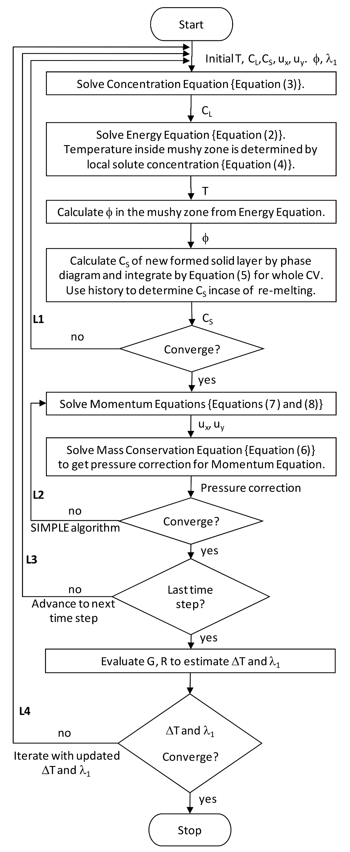
3.4. Numerical Simulation Procedure

One of the novelties of the numerical algorithm proposed in this study is the incorporation of ΔT during solidification in our simulations. Before the details of the numerical simulation procedure are presented, an overview of the methods developed to incorporate ΔT in the simulation is presented below.

Figure 4 presents a schematic of the steps during uni-directional solidification of the liquid from an initial melt superheat temperature of T_ini to the final eutectic temperature of T_eut.

Table 2. The various steps in the solidification of a CV of a binary alloy.

Steps	Time	T	CS (New Layer)	CL	Figure
Step 1	0 to t1	Tini to Tliq	0	Co	Figure 4b,c
Step 2	t2	Tliq to (Tliq − ΔT)	kCL1(≅kCo)	$\mathrm{C}{\mathrm{L}}_1 < {\mathrm{C}}_{\mathrm{L}}^{\ast }$	Figure 4d
Step 3	(t2 + Δt)	(Tliq − ΔT) (no change)	kCL2	$\mathrm{C}{\mathrm{L}}_2 < {\mathrm{C}}_{\mathrm{L}}^{\ast }$	Figure 4e
Step 4	t*	(Tliq − ΔT) (no change)	kCL*	${\mathrm{C}}_{\mathrm{L}}^{\ast }$	Figure 4f
Step 5	t3	T3 < (Tliq − ΔT)	kCL3	$\mathrm{C}{\mathrm{L}}_3 > {\mathrm{C}}_{\mathrm{L}}^{\ast }$	Figure 4g
Step 6	tn	Teut	Ceut	Ceut	Figure 4h
Step 7	tfinal	Teut	Ceut	Ceut	Figure 4i

shows the steps involved during solidification of a binary hypoeutectic alloy. In this study, all these steps were considered in each CV during solidification simulation.

A detailed description of each step is also given below:

Step 1. T_ini decrease to T_liq (Figure 4b,c) mainly due to the heat extraction during solidification. Concentration of the alloy melt is maintained at C_o. The time taken for this step is t₁.

Step 2. No solidification event occurs at T_liq. The first solid appears after an undercooling of ΔT as shown in Figure 4d. The extent of undercooling is evaluated by Equation (1). The concentration of the first solid phase is represented by kC_L1 wherein the liquid concentration C_L1 is marginally greater than the average alloy composition C_o. The time taken for this step is t₂.

Step 3. During the next time step (t₂ + Δt), the temperature remains constant as that in Step 2 (T_liq − ΔT). Evolution of the primary phase occurs during this step and the temperature will continue to remain constant (latent heat of fusion balances the heat extraction) until the solute concentration in the liquid at the mushy zone/liquid interface reaches ${\mathrm{C}}_{\mathrm{L}}^{\ast }$ as shown in Figure 4a,e.

Step 4. The solute concentration of the liquid at the mushy zone/liquid interface reaches ${\mathrm{C}}_{\mathrm{L}}^{\ast }$ in time t* and the solute concentration in the solid is given by ${\mathrm{kC}}_{\mathrm{L}}^{\ast }$ as shown in Figure 4a,f.

Step 5. The temperature begins to decrease again and layers of solid of the primary phase are formed at composition and the solute re-distribution in the liquid phases is defined by the concentration equation given by Equation (3), as shown in Figure 4g. The solute concentration in the all layers of solid of primary phase is evaluated by Equation (5) for each time step if there is no re-melting of the solid phase due to convection of the liquid. In case re-melting occurs, the history of the solute concentration in the solid is used to evaluate the average concentration of the solid inside CV [10,11].

Step 6. Temperature of the liquid reaches the eutectic temperature and a layer of solid with eutectic solute concentration is formed marking the end of growth of the primary phase, as shown in Figure 4h.

Step 7. The remaining liquid at the eutectic temperature is transformed into a two-phase mixture to complete the solidification of the CV, as shown in Figure 4i.

The unique feature in this model is the Steps 2 to 4 where the temperature of the CV is maintained at T_liq − ΔT until the solute concentration in the liquid inside CV reaches the equilibrium concentration of the solute, ${\mathrm{C}}_{\mathrm{L}}^{\ast }$, as suggested in Figure 4a. This is observed during the solidification process of all binary alloys; however, the event has never been accounted for in any solidification simulation of binary alloys until this study. Introducing Steps 2 to 4 will identify and account for the time period of thermal recalescence during solidification.

Table 3. Notations and details of the solidification simulations.

Simulation Identification	Type	Co	ΔT
SA	Upward Solidification	Al-3wt%Si	0
SB
S1	Upward Solidification	Al-3wt%Si	0
S2			Equation (1)
S3		Al-7wt%Si	0
S4			Equation (1)
S5	Downward Solidification	Al-5wt%Si	0
S6			Equation (1)
S7		Al-7wt%Si	0
S8			Equation (1)

presents the identification and details of the simulations in this study.

Typical deliverables from the simulations listed in Table 3 include transient temperature distribution and solidification time for the mushy zone/liquid interface, as well as other quantified parameters such as λ₁, G and R. In the governing equations (Equations (2), (3) and (6)–(8)), the central differencing scheme was employed for all the diffusion terms; the convection terms were discretized by hybrid difference scheme. The implicit method was used for the transient terms. Convergent criteria for all parameters were determined by the two orders of mesh size, since the numerical simulation in the present study is in two orders of accuracy.

Figure 5 presents the process flow chart for the numerical simulations: there are four procedural loops, L1, L2, L3 and L4. At every time step, Equations (2)–(5) are processed in L1 to evaluate the transient temperature distribution, solute concentration distributions in both the liquid and solid phases, and ϕ in the mushy zone. Equations (6)–(8) are processed in L2 to obtain the velocity distribution of liquid (fluid flow) using the algorithm defined by the Semi-Implicit Method for Pressure-Linked Equations (SIMPLE) [33]. Momentum equations (i.e., Equations (7) and (8)) are solved using an initial pressure field. The pressure field is corrected using the mass balance equation (Equation (6)). By iterating these two major steps, a convergent solution for velocity and pressure fields can be obtained. Each time step is then advanced with L3 and ΔT and λ₁ are evaluated using the loop L4. The loop L4 enables the evaluation of λ₁ while incorporating the undercooling, ΔT at the macro-level (CV ~ 1 mm) solidification simulation. Previous researchers could not introduce loop L4 to predict microstructure features such as λ₁ because of the lack of valid correlations of the transient temperature distribution and solidification time with experiments. Prior to incorporating the loop L4, the optimization of critical parameters such as thermo-physical properties as a function of temperature, shrinkage, fluid flow from natural convection and undercooling were carried out with several preliminary simulations to enable experimental validation of the transient temperature distribution and solidification times during solidification.

The main feature of the algorithm presented in Figure 1 is the procedural logic used in loop L1 shown in Figure 5:

• At time step t = t_m, Equation (3) was used to evaluate the distribution of solute concentration in all of liquid, solid and the two-phase mushy zone.
• Solving Equation (2) and comparing the evaluated T of each CV to (T_liq − ΔT), the CV was determined to be in either the liquid phase or mushy zone.
• Equation 4 was used to evaluate temperature distribution inside the mushy zone or assumed as (T_liq − ΔT) if C_L < ${\mathrm{C}}_{\mathrm{L}}^{\ast }$ (Figure 4d–f). Equation (2) was used to evaluate the temperature distribution inside the liquid and solid phases.
• The temperature distribution, evaluated from Equation (2) was used to evaluate ϕ in the mushy zone.
• If there is no re-melting of the solid in any given CV, Equation (5) was used to calculate the mean solute concentration of the solid phase in the CV, and in case of solid phase re-melting in any given CV, the history of prior mean solute concentration in the solid phase was used for the current time step [10].
• All the above steps were repeated until convergence.

In any given CV in the domain, the temperature of the CV to determine if it is presented in either the entirely liquid or solid phase regimes of the domain was evaluated by the energy equation, Equation (2); meanwhile, the temperature in the two-phase mushy zone was evaluated by the Equation (4) with local equilibrium assumption. To determine, if the given CV falls within the mushy zone, the temperature of the liquid in that CV was evaluated using Equation (2) and if this temperature value is less than T_liq, then the temperature within that CV is re-evaluated using Equation (4). Further, this temperature of the liquid in a CV in the mushy zone was input back in the Equation (2) to calculate ϕ in the mushy zone. This procedure in the first iterative process does not include the undercooling (ΔT = 0) and hence, the first iteration of loop L4 would have been carried out with ΔT = 0; meanwhile, subsequent iterations of L4 will yield a positive value for ΔT and updated values of the temperature distribution in the CV.

The novelty of the algorithm presented in this study, wherein the energy and solute concentration equations were coupled, is in the loop L1. The advantages of loop L1 in this new algorithm (Figure 5) over that by Felicilli et al. [10] (Figure 1) that enabled the incorporation of the undercooling term, ΔT are in two aspects: firstly, the former solves the solute concentration equation first for all the three regimes of liquid, solid and mushy zone to circumvent the instabilities caused by the phase transformation term in the energy equation, Equation (2), and secondly, the new algorithm uses the heat transfer condition, solely, to evaluate the ϕ in the mushy zone. As a result, a significant reduction in the computational time was realized from using this newly proposed algorithm as well.

In summary, the advantages of the new algorithm for solidification simulation of binary alloys over the existing ones are the ability to incorporate the undercooling at the liquid/mushy zone interface, ΔT, overcome the instabilities caused by the phase transformation term in the energy equation due to strong non-linearity and significant reduction in computation cost. Further, a successful and complete correlation of the simulations by experiment results was also carried out to ensure its validity.

4. Results and Discussion

All the results and discussion are in reference to Figure 2 and Figure 5. The results and discussion are presented for the following topics:

• Comparison of new algorithm with the popular version.
• Transient temperature distribution.
• Effect of ΔT on solidification time.
• Effect of ΔT in the liquid on fluid flow.
• Effect of ΔT in the liquid on G.
• Effect of ΔT in the liquid on R.
• Effect of ΔT in the liquid on λ1.

4.1. Comparison of New Algorithm with the Popular Version

The results at the end of the first iteration of L4 in Figure 5 are presented as simulation SA and were used to compare with the results from the popular algorithm (simulation SB) [10,11,12] to determine the reliability of this newly proposed algorithm (shown in Figure 1 and Figure 5).

Comparison of the transient temperature distribution for SA obtained in the present study at the end of the first iteration of L4 in Figure 5 and that SB simulated by the algorithm presented in Heinrich et al. [11] (Figure 1) is reported in Figure 6.

Figure 6 shows the temperature distribution at r = 0 during solidification without the effect of ΔT for seven locations between y = 0 and y = 84 mm, respectively; also shown is the comparison between the present work and that of Heinrich et al. [11] showing that using the new algorithm proposed in this study is as accurate as the popular method which indicate that the alternative logic used to determine ϕ from solely the heat transfer conditions rather than the concentration equation is valid. Further, the computing time for the new algorithm to obtain the results shown in Figure 6 was reduced by a maximum of 50% depending on the initial solute concentration of the alloy and boundary conditions. The average cooling rates investigated in Figure 6 varied between 0.72 °C/s to 2.05 °C/s.

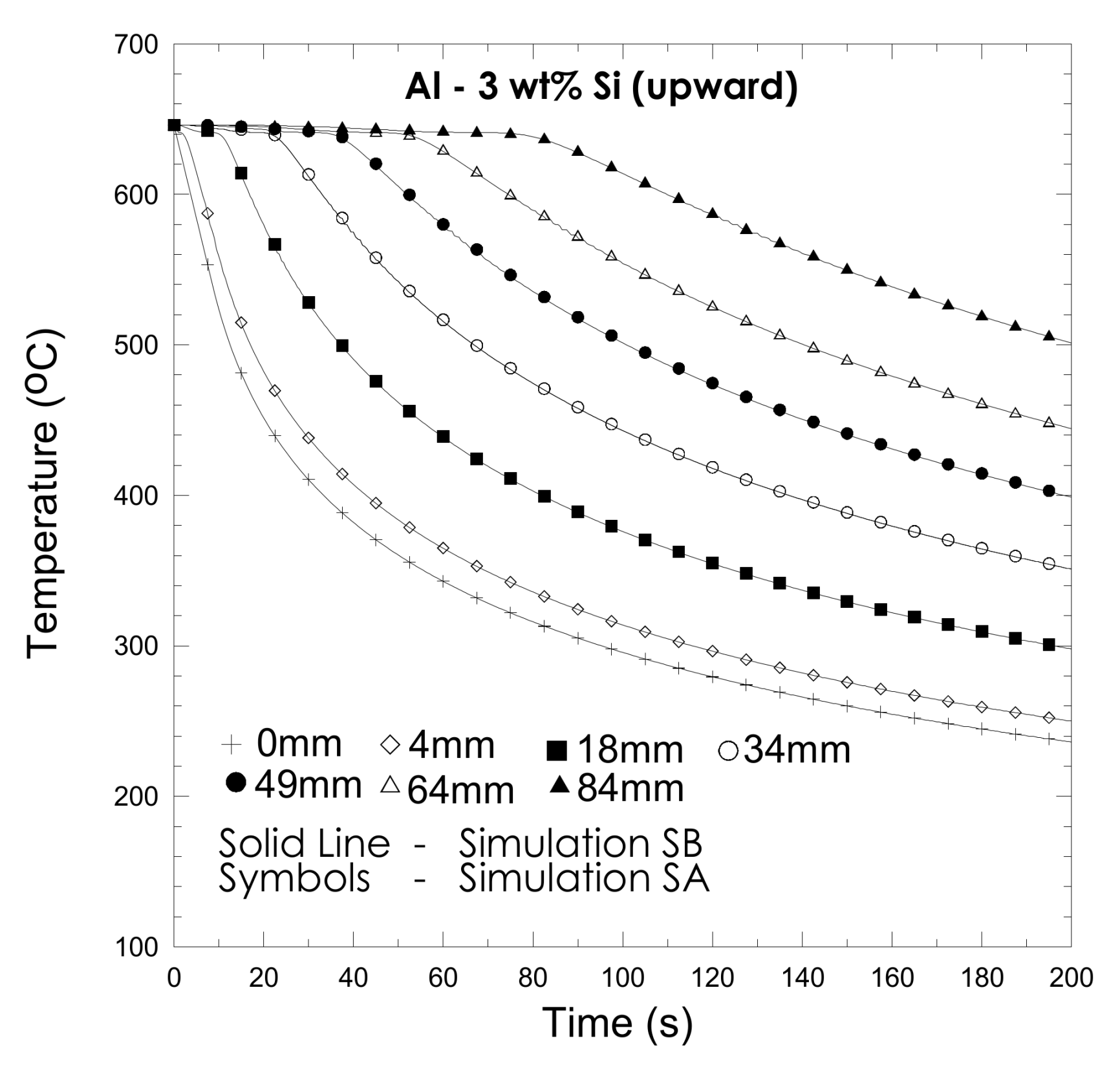
4.2. Transient Temperature Distribution

Transient temperature distribution is critical to evaluate solidification time, G, R and λ₁. The transient temperature distribution in the computing domain was validated with experiment results presented by two groups of researchers [18,30]. Figure 7a,b show the validation of the present algorithm using the experiments by Peres et al. [18] and Spinelli et al. [30]. Figure 7a,b are for simulations S2 and S8, respectively. Simulations S2 and S8 show a good agreement with experiments and validate the numerical method. In Figure 7a, the maximum deviation in temperature is less than 10 °C located at y = 64 mm and t ≈ 100 s for upward solidification. When compared with the initial melt temperature of 644.05 °C, the deviation is less than 2%. In Figure 7b, the maximum deviation is less than 13 °C (2%) located at y = 64 mm and t ≈ 100 s for downward solidification.

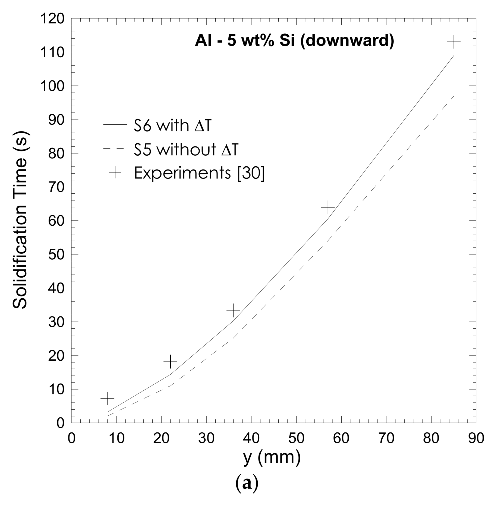
4.3. Effect of Undercooling on Solidification Time

Peres et al. [18] have carried out experiments on upward solidification (Figure 2a) with Al-3wt%Si and Al-7wt%Si alloys, respectively. They have reported the solidification time (location of the mushy zone/liquid interface) by estimating the time taken for the interface to reach the location of each thermocouple in the experiments. These experiments were used to validate simulations S2 and S4. Figure 8 shows the results of these validations.

Figure 8a shows the validation of the solidification times from simulation S2 (with ΔT) with the experiments [18] along with results from S1 (no ΔT). Figure 8b shows the validation of the solidification time from simulation S4 (with ΔT) with the experiments [18] along with results from S3 (no ΔT). Figure 8 shows that the simulations that include the effect of ΔT on solidification has an excellent agreement with the experiments with a maximum time deviation of <1.5% for the farthest thermocouple (y = 84 mm) in both Figure 8a,b (refer to Figure 2a). The deviation may be due to the lack of uni-directional heat transfer in the experiments towards the later stages of solidification. However, the negligible deviation shows that experiments were nearly uni-directional for most of the solidification time. It can be seen in Figure 8a,b that simulations S1 and S3 with no consideration of ΔT during solidification have a large deviation from the respective experiments. The maximum time deviation in S1 and S3 from experiments is 11.4% and 19.8%, respectively, at y = 84 mm. In Al-3wt%Si alloy, the total time taken for the mushy zone/liquid interface to travel between y = 0 to y = 84 mm is 88 s from experiments, 86.7 s for S2; and 78 s for S1. In Al-7wt%Si alloy, the total time taken for the mushy zone/liquid interface to travel between y = 0 to y = 84 mm is 96 s from experiments, 94.7 s for S4; and 77 s for S3. The consideration of ΔT in the simulation reduces the velocity of the liquid/mushy zone interface, R because it requires longer time for each CV to reach an undercooled temperature state (T_liq − ΔT) before any solidification event.

Spinelli et al. [30] have carried out experiments on downward solidification with Al-5wt%Si and Al-7wt%Si alloys. The results from these experiments were used to validate simulations S6 and S8. Figure 9a,b shows the validation of simulation S6 and S8. Additionally shown in Figure 9a,b are the solidification times for simulations S5 and S7. Figure 9 shows that simulations S6 and S8 (with ΔT) have better agreement with the experiment results. The maximum deviation of S6 and S8 from experiments at y = 85 mm is 3.6% and 16%, respectively. The larger deviations from the experiments observed for the downward solidification in Figure 9 as compared with the upward solidification presented in Figure 8 may be due to the fact that in experiments [18,30], the temperature gradient between the side wall of the container (right side of computing domain) and the liquid alloy inside increases with time in the experimental condition. In downward solidification, the fluid flow is more pronounced due to the natural convective currents induced by this temperature gradient in experiments, which results in a more significantly increased temperature gradient in the liquid side of mushy zone/liquid interface causing a smaller value of R and longer solidification time in downward solidification in experiments. Another reason for the marginal under prediction of solidification times in Figure 8 and Figure 9 may be due to the added latent heat of fusion of the eutectic phases which will result in an over prediction of R and an under-prediction of the solidification times. In Al-5wt%Si alloy, the total solidification times for experiment, S6 and S5 are 113 s, 109 s and 97 s, respectively. In Al-7wt%Si alloy, the total solidification times for experiment, S8 and S7 are 130 s, 108 s and 96 s, respectively.

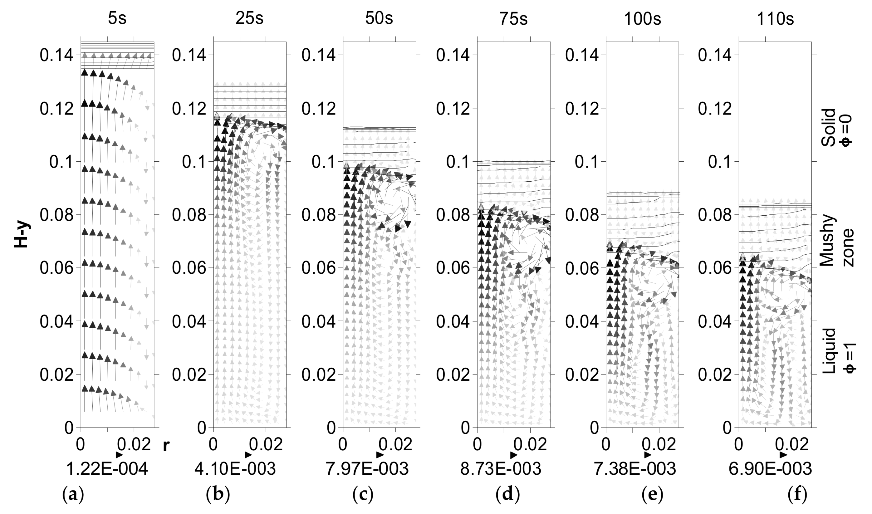
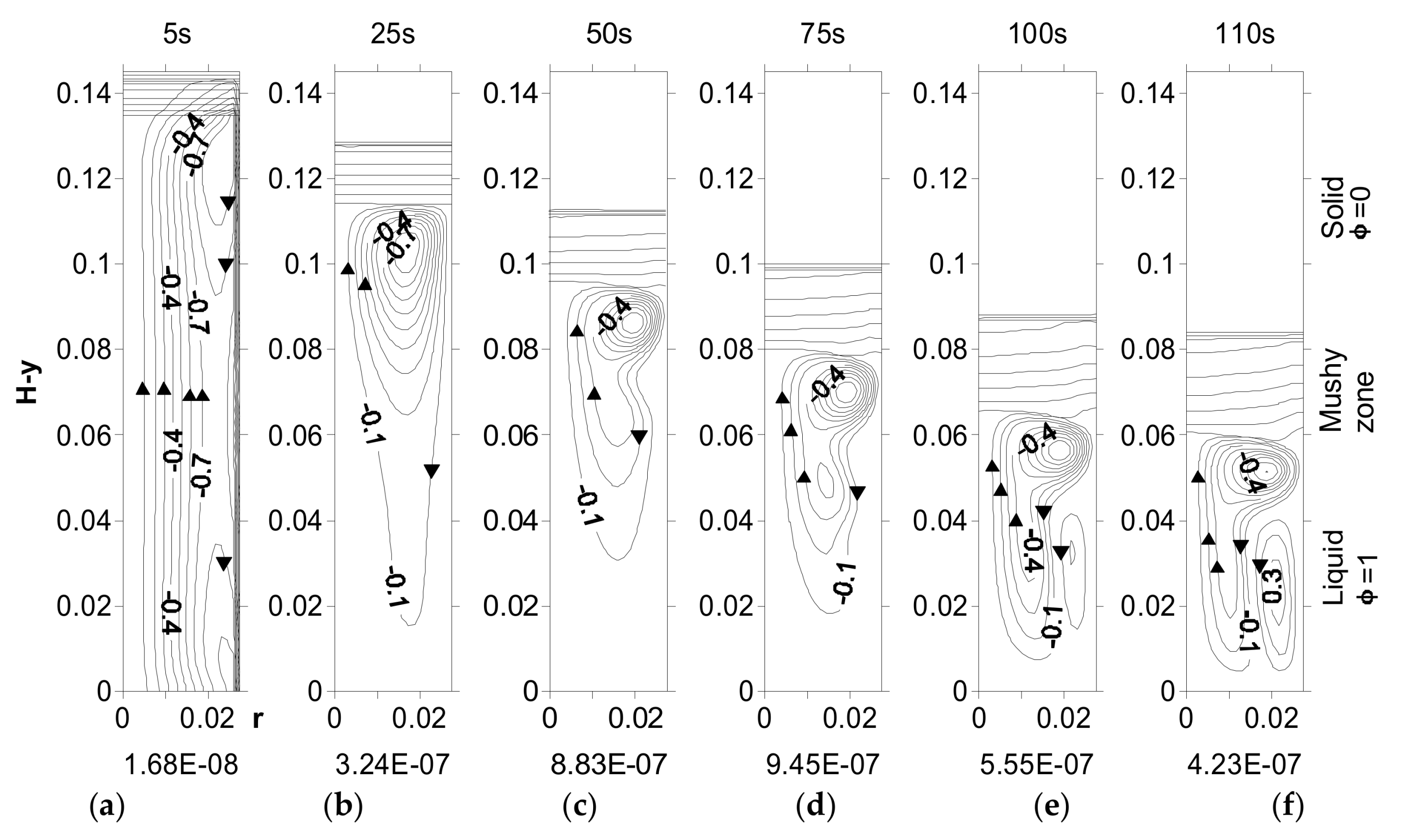
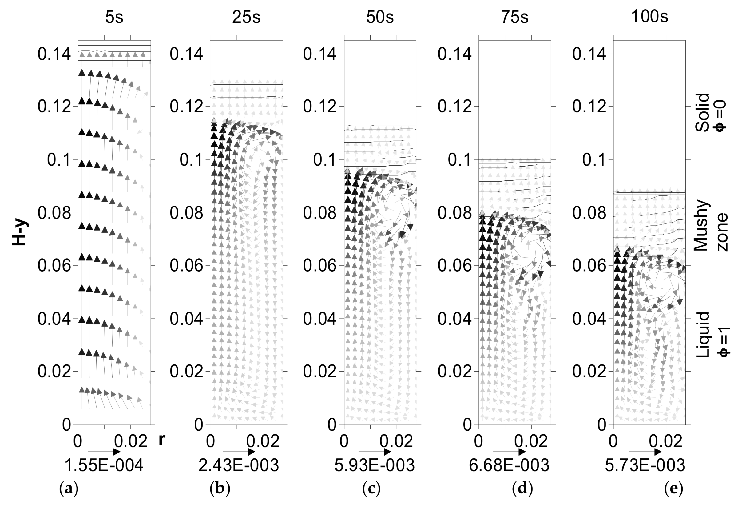
4.4. Effect of Undercooling on Fluid Flow—Upward Solidification

Figure 10a–c presents the velocity profiles (m/s) for simulation S2 and Figure 10d–f present that for simulation S1. In these two simulations (upward solidification) the positive density gradient is in the direction of the gravity vector (refer to Figure 3a) and hence, there will be no natural convection of the liquid which is evident from fluid flow from top to bottom and the absence of circular flow. Since only shrinkage affects the fluid flow velocities and shrinkage is almost identical in both simulations, S2 and S1, there is a marginal increase in the velocity of S1 (without ΔT) as compared to that in S2 (with ΔT) due to the larger value of R in S1. A similar observation was made when simulation S4 was compared with S3 as well.

4.5. Effect of Undercooling on Fluid Flow—Downward Solidification

The development of fluid flow with the effect of undercooling for simulation S6 is shown in Figure 11. Figure 11a,f show snapshots of the velocity field in the computing domain at increasing solidification times of 5 s, 25 s, 50 s, 75 s, 100 s and 110 s, respectively. Maximum magnitude of the velocity at each time is shown at the bottom of the respective snapshot. Figure 11f shows typical domains found in the simulation results: solid, mushy zone and liquid. The solid lines inside the mushy zone in Figure 11 represent the constant ϕ lines from ϕ = 0.9 to ϕ = 0.1.

Table 4. Development of fluid flow for simulation S6.

Time (s)	Maximum Velocity (mm/s)	Flow due to Shrinkage	Flow due to Natural Convection	Height of the Mushy Zone (mm)
5	1.22 × 10−4	Dominant flow from bottom to top	Small circular flow limited to mushy zone/liquid interface around r = 27.5 mm	13
25	4.1 × 10−3	Small effect of shrinkage in liquid. Large effect of shrinkage in mushy zone.	Dominates the liquid. Small effect in mushy zone.	20
50	7.97 × 10−3		Strengthens in liquid.	23
75	8.73 × 10−3		Strengthens further in liquid.	24
100	7.38 × 10−3		Weakens in liquid.	28
110	6.9 × 10−3		Further weakens in liquid.	31

presents a summary of the results shown in Figure 11. Table 4 suggests that effect of shrinkage is dominant at the beginning of solidification due to the lack of natural convection. The effect of natural convection gradually begins to dominate and the effect of shrinkage on fluid flow velocity becomes negligible as solidification time increases. At the beginning of solidification, R is high and induces an instantaneous flow field in the liquid which is primarily caused by the solidification shrinkage. However, the flow due to the density gradient in the liquid develops from an initial rest to subsequently dominate the fluid flow regime over the solidification shrinkage.

Higher velocities of fluid flow caused by natural convection will result in greater circular flow regions, as seen in Figure 11. There are two mechanisms that affect strength of fluid flow due to natural convection. One of them is the density gradient caused by the temperature and solute concentration gradients in the liquid which is directly proportional to the fluid velocity and the other is the height of the liquid (space available for fluid flow) which is inversely proportional to fluid velocity. Between times t = 5 s and 75 s, the effect of the density gradient greatly increases the fluid flow velocity due to natural convection. However, between t = 75 s and 110 s the effect of the reducing height of the liquid marginally decreases the fluid flow velocity due to natural convection. The maximum fluid flow velocity is always in the region close to r = 0 and is in the direction of heat extraction. Figure 11 and Table 4 also show that the length of the mushy zone is continuously increasing indicating an unsteady solidification condition at all times because of the continuously decreasing heat flux $\overrightarrow{q}$ at y = 0 mm.

The maximum flow in the computing domain can always be observed at the left top of the liquid region from Figure 11b,f (center of the solidifying cylinder). Fluid flow with a higher temperature from liquid region is driven into mushy zone in this region. Therefore, solidification time will increase in this region and hence the constant liquid fraction lines are compressed along the y direction at the liquid/mushy zone interface (Figure 11b–f). The direction of the fluid flow velocity at the liquid/mushy zone interface is predominantly in the positive r direction due to the development of clockwise fluid flow: resulting in the accumulation of enthalpy on the top ride side of the liquid region (along the wall of the solidifying domain). As a result, solidification in this region is slowed down and the constant liquid fraction lines along the wall are also compressed as shown in Figure 11d–f.

The normalized iso-stream function lines with the effect of undercooling in simulation S6 are shown in Figure 12. Figure 12a–f shows snapshots of the normalized iso-streamlines in the computing domain at increasing solidification times of 5 s, 25 s, 50 s, 75 s, 100 s and 110 s, respectively. Maximum magnitude of stream function is shown below each snapshot for the respective times. Similar to Figure 11, the top solid lines inside the mushy zone in Figure 12 represent the constant liquid fraction lines from ϕ = 0.9 to ϕ = 0.1. The strength of fluid flow can also be implied by the maximum magnitude of stream function. Maximum magnitude of the stream function in Figure 12 changes from a lower value (Figure 12a) to a maximum value (Figure 12d) and back again to a lower value (Figure 12f), which indicates the strength of flow develops from weaker to stronger and back to weaker as the solidification proceeds. Arrows in the streamlines in Figure 12 illustrate the flow direction, which indicates that flow develops from bottom to top at t = 5 s. Circular flow developed after t = 25 s implies that the flow is dominated by natural convection. Clockwise cell can be observed for times between t = 25 and 75 s. After t = 100 s, a second flow cell is created at the right bottom side of the computing domain due to the higher velocity at t = 75 s during the development of the fluid flow. A notable feature is the development and strengthening of a secondary circular flow starting from t = 75 s as shown in Figure 11 and Figure 12.

Figure 13a–d show the velocity distribution in both y and r directions at t = 5 s and t = 50 s for simulation S6, respectively. As shown in Figure 13a,b for velocities at t = 5 s, the maximum magnitude of u_y is more than 10 times that of u_r, which indicates that the flow is dominated by shrinkage.

Positive direction of u_y located at the region close to the right side of computing domain (wall of solidifying cylinder) implies that natural convection has already affected fluid flow even if it has not dominated the flow pattern at t = 5 s. The flow in the middle of the solidifying cylinder in the y direction is nearly fully developed as indicated by the lack of variation in the magnitude of u_y and u_r at locations (H-y) = 0.04 m, 0.06 m and 0.08 m in Figure 13a,b, respectively. The higher variation in the magnitudes of velocities in Figure 13a,b at locations (H-y) = 0.01 and 0.113 m is due to the effect of the cavity end walls. In Figure 13c,d, the lack of significant variation between the maximum magnitudes of u_y and u_r at time t = 50 s show that the flow is circular and caused predominantly by natural convection. At t = 50 s, the maximum velocity is located near the liquid/mushy zone interface at a location close to the left side of the computing domain.

Figure 14 shows the development of fluid flow of simulation S5 (no effect of ΔT on solidification). Comparing Figure 11 with Figure 14 shows that the nature of development of fluid flow dominated by shrinkage initially and subsequently dominated by natural convection are similar. However, the only difference is in the magnitude of the fluid flow velocities at the various time steps.

Table 5. Comparison of maximum fluid flow velocities between simulations S6 and S5.

Time (s)	Maximum Velocity (m s−1)
	S6 (with ΔT)	S5 (without ΔT)
5	1.22 × 10−4	1.55 × 10−4
25	4.1 × 10−3	2.43 × 10−3
50	7.97 × 10−3	5.93 × 10−3
75	8.73 × 10−3	6.68 × 10−3
100	7.38 × 10−3	5.73 × 10−3

shows a comparison of the magnitude of fluid flow velocity between simulations S6 and S5.

Due to the absence of ΔT in S5, the temperature gradient in the liquid ahead of the mushy zone/liquid interface is always less than that in S6. Hence, the value of R in S5 is always greater than that in S6. In the beginning of solidification, the higher value of R will cause a larger effect of shrinkage on the fluid flow velocity as reflected by the higher magnitude of velocity at t = 5 s as shown in Figure 14 and Table 5. However, due to the lower temperature gradient in S5, the solute density gradient in the liquid is lower than that in S6 at t ≥ 25 s, which will result in a lower fluid flow velocity due to natural convection in the liquid in S5 as shown in Figure 14 and Table 5. This underestimation of fluid velocity due to natural convection in S5 as compared to S6 will greatly affect the evaluation of λ₁ as will be discussed in subsequent sections of this manuscript.

The normalized iso-stream function lines without the effect of ΔT for simulation S5 are shown in Figure 15. Figure 15a–e shows snapshots of the normalized iso-streamlines in the computing domain at increasing solidification times of 5 s, 25 s, 50 s, 75 s, 100 s, respectively. Maximum magnitude of stream function is shown below each snapshot. The difference between the flow field shown in Figure 15 (without effect of ΔT) and that shown in Figure 12 (with effect of ΔT) is best indicated by the difference in the maximum magnitude of the respective stream functions. As shown in Figure 12a and Figure 15a, a higher magnitude of stream function for simulation S5 implies stronger fluid flow at t = 5 s. After the initial stage of solidification, results from simulation S6 always have higher magnitudes of maximum stream function due to the stronger buoyancy flow caused by the higher-density gradient in the liquid region with ΔT. The weaker fluid flow due to the negligence of the effect of ΔT in solidification (Figure 15) results in a delay in the development of the secondary circular flow cell in the liquid when compared to the simulation S6 with the effect of ΔT (Figure 12).

Figure 16a–d shows the velocity distribution in both y and r directions at t = 5 s and t = 50 s for simulation S5, respectively. Distribution of velocities in either r or y direction in Figure 16 is similar to the results shown in Figure 13. It is found that higher magnitudes of velocity could be obtained in simulation S5 at t = 5 s. However, stronger fluid flow can be observed at t = 50 s in simulation S6.

Figure 17a,d shows the distribution of fluid flow velocity for simulation S8 and Figure 17e–h show that for simulation S7. The comparison of velocity distributions between S8 and S7 is similar to that observed in S6 and S5. With the same line of reasoning as presented for S6 and S5, it can be observed that when ΔT is not considered during solidification (S7) the maximum velocity at the beginning of solidification is almost the same as that with ΔT (S8) (compare Figure 17a,e) because fluid flow induced by shrinkage dominates over that induced by natural convection. However, at larger time intervals, the velocities of S7 are lower than that of S8 because the effect of natural convection is more on the fluid flow velocities due to ΔT (compare Figure 17b–d with Figure 17f–h, respectively).

5. Effect of Undercooling on G

Figure 18 shows the distribution of the temperature gradient, G in the liquid ahead of the mushy zone/liquid interface. There are two main reasons for the decrease in the value of G with increasing solidification time: one is the decrease in the heat flux at the heat extraction boundary with time and the other is the decrease in the bulk temperature of liquid with time. Figure 18a,b shows the results for simulations Al-3wt%Si (S1 and S2) and Al-7wt%Si (S3 and S4) alloys, respectively; and Figure 18c,d are for Al-5wt%Si (S5 and S6) and Al-7wt%Si (S7 and S8) alloys, respectively. Since the temperature of the mushy zone/liquid interface will be lower when we consider the undercooling, ΔT, the value of G is higher for the solidification simulations with the effect of ΔT included (S2, S4, S6 and S8) than that in those without the effect of ΔT (S1, S3, S5 and S7) for the respective alloys. In Figure 18a,b (upward solidification), G decreases during the solidification process. In Figure 18c,d (downward solidification), there seem to be three distinct regions from the beginning to end of solidification. These regions are marked by line segments AB, BC and CD in all the curves in Figure 18c,d.

Table 6. Locations A, B, C and D shown in Figure 9c,d along with the solidification parameters at each location.

Simulation	ΔΤ	Interface Location y (mm)	Solidification Time (s)	Maximum Fluid Flow Velocity (mm.s−1)	Variation in Maximum Velocity	G (K.mm−1)
S5 (Al-5wt%Si)	0	8(A)	2	0.16	none	0.6
		22(B)	11	0.37	131%	0.3
		36(C)	25	2.43	557%	0.24
		85(D)	97	5.95	145%	0.03
S6 (Al-5wt%Si)	Equation (3)	8(A)	3.2	0.16	none	0.9
		22(B)	14.4	0.47	194%	0.49
		36(C)	30.3	5.68	1109%	0.55
		85(D)	108.9	6.95	22%	0.16
S7 (Al-7wt%Si)	0	8(A)	3.6	0.07	none	0.58
		22(B)	13	0.68	871%	0.34
		36(C)	27	3.03	346%	0.31
		85(D)	95.6	7.65	152%	0.02
S8 (Al-7wt%Si)	Equation (3)	8(A)	5.4	0.07	none	0.9
		22(B)	16.8	0.99	1314%	0.6
		36(C)	32.8	10	910%	0.77
		85(D)	107.3	8.35	−17%	0.15

presents the four locations A, B, C and D of the mushy zone/liquid interface, solidification times, maximum fluid flow velocity, variation of fluid flow velocity from previous location and the temperature gradient, G in the liquid at the mushy zone/liquid interface at each location.

As discussed in the previous section on the effect of ΔT on fluid flow during downward solidification (refer to Figure 11, Figure 12, Figure 13, Figure 14, Figure 15, Figure 16 and Figure 17 and Table 6), the fluid flow in the initial stages of solidification as defined by line segment AB is dominated by shrinkage. Between points A and B, the decrease in G is only due to the decrease in the heat extraction rate between these locations. Between points B and C, the strong positive density gradient develops against the direction of the gravity vector and causes a significant increase in the fluid flow velocity due to natural convection.

In simulation S5 (no ΔT) the change in the velocity between B and C is 557% and that in S6 (with ΔT) is much higher at 1109% because the consideration of ΔT will enhance the fluid flow velocities due to larger density gradients. This increase in velocity between B and C in both S5 and S6 will cause a tendency to increase the magnitude of the gradient of G (Figure 18c and Table 6). In S6, the velocity change is so drastic due to the added effect of ΔT and there is an increase in the value of G between locations B and C. The same argument can be made for the change in G between locations B and C for simulations S7 and S8 as well (Figure 18d and Table 6).

5.1. Effect of Undercooling on R

Figure 19 shows the distribution of the solidification velocity, R at r = 0 and various locations of y = 0 to 84 mm in the computing domain (Figure 3). The value of R was estimated by the velocity of the mushy zone/liquid interface during solidification. Figure 19 shows the value of the velocity of the mushy zone/liquid interface (ϕ~0.999) velocity, R. Figure 19a,d shows the results for solidification simulation for Al-3wt% (upward), Al-7wt%Si (upward), Al-5wt%Si (downward) and Al-7wt%Si (downward), respectively. Figure 19 shows that for all the simulations transient value of R decreases overall with increasing distance from the heat extraction interface because the magnitude of heat flux at the heat extraction boundary and the computing domain decreases with time as the volume of the solid phase increases.

In all results shown in Figure 19, the value of R evaluated with the effect of ΔT is always lower than that without the effect of ΔT because the introduction of ΔT will require a lower temperature for the solidification than the T_liq, which will cause a delay in the solidification event. The value of R is high at the beginning of solidification for all the simulations in Figure 19. The effect of undercooling on R is more pronounced at the earlier stages of solidification. In Figure 19a,d, the maximum deviation in the estimated value of R at 8 mm from the heat extraction interface is 18%, 89%, 33% and 26%, respectively. In Figure 19c,d, the value of R for simulations S5 and S7 (no ΔT) increase towards the end of solidification of the computing domain because, without the effect of ΔT for downward solidification, the value of G will decrease more significantly towards the end of solidification and result in an increase in R (between y = 58 mm to y = 84 mm). For upward solidification in simulations S1 and S3 (Figure 19a,b), the value of G does not decrease enough to cause an increase in R. If one considers the effect of ΔT during downward solidification as in simulations S6 and S8 in Figure 19c,d, the value of G will be greater than those without the effect of ΔT, as shown in Figure 18c,d, and will not decrease so low to as to increase the value of R.

5.2. Effect of Undercooling on the Estimation of λ₁

Figure 20a,b show the distribution of the primary dendrite arm spacing, λ₁ as a function of cooling rate (G.R) of the liquid at the mushy zone/liquid interface. It can be observed that there is no significant change in the value of (G.R) between the simulations with the effect of ΔT (simulations S2 and S4) and that without (S1 and S3), respectively, because the effect of ΔT will increase the value of G but simultaneously decrease the value of R and hence the product (G.R) will remain fairly unchanged. Additionally shown in Figure 20a,b are the values of λ₁ from the experiments in upward solidification from Peres et al. [18]. It can be seen that simulations S1 to S4 predict the respective values of λ₁ with a reasonable accuracy. There is a slight under-prediction of the value of λ₁ because of a combination of two reasons: the model (Equations (1) and (2)) itself is semi-empirical for an unsteady state solidification process and hence may tend to over-predict or the cooling rates of the mushy zone/liquid interfaces were measured after the liquidus temperature was recorded by the thermocouples in the experiment [18] and the magnitude of this value will be higher than the actual cooling rate at the mushy zone/liquid interface and will result in an over-prediction of (G.R) in the experiments, as shown in Figure 20a,b. If the value of (G.R) is being over-predicted by the experiment results, then the value of λ₁ should be under-predicted (Equation (1)) as it is shown as function of location (Figure 21a) for simulations S1 and S2. In Figure 21a, the value of (G.R) at any specific location (Figure 3) will be higher when the effect of ΔT is considered than that without the effect. Hence, the value of λ₁ obtained at any specific location will be lower in simulations with the effect of ΔT than in those without the effect. Hence in Figure 21a, the simulation S2 (with ΔT) predicts the value of λ₁ more accurately than that by S1 (without ΔT).

Figure 20c,d shows the distribution of λ₁ as a function of (G.R) for the cases of downward solidification in simulations S5 to S8. As discussed previously about the effect of ΔT on G in the downward solidification, there are three distinct regions wherein the magnitude of the value of gradient of G decreases at the first region and increases at the second region (fluid flow dominated by the emergence of density gradient causing significant increase in fluid flow velocities than that caused by shrinkage in the first region) and again decreases at the third regions. The trend of λ₁ will also follow the trend of G in these three regions as in Figure 20c,d. The value of λ₁ increases (G decreases) in the first region between points A and B, then λ₁ decreases when the magnitude of gradient of G increases in the second region between points B and C and subsequently when the fluid flow velocities due to density gradient is stabilized in the third region, the value of λ₁ again increases between points C and D in both simulations with and without the effect of ΔT. However, the effect of undercooling, ΔT, on the magnitude of the fluid flow velocities in the three regions will have a greater effect on the changes in the value of G in the three regions and hence a greater effect on the value of λ₁ in these regions as well (refer to Equation (11)). Figure 20c,d also shows that the λ₁ estimated in the experiments by Spinelli et al. [30] seems to be closer to the values predicted by the simulations with the effect of ΔT included.

The values of λ₁ in the first region in alloy Al-5wt%Si (simulations S5 and S6) between points A and B seem to be under-estimated by the experiments and this may be due to various errors in the experiment evaluation of the cooling rate at the mushy zone/liquid interface and λ₁ caused by the high value of R in this region. Further, the decrease in λ₁ between points B and C can be observed from the experiment results as predicted by the simulations in Figure 20c [30]. Experiments will have to be carried out to obtain more data points in this region to validate the simulation results. Figure 21a,b show the distribution of the value of λ₁ as a function of location (refer to Figure 3) for Al-3wt%Si upward and Al-5wt%Si downward solidification, respectively. These show a better prediction of the λ₁ by the simulation with the effect of ΔT than the one without. The anomalous behavior of the trend in λ₁ can also be observed in the second region between points B and C in Figure 21b. It is due to the development of the higher fluid flow velocities caused by the emergence of the density gradients causing natural convection in the computing domain.

6. Summary and Conclusions

A new and more efficient algorithm to simulate the solidification of binary alloys that includes the effect of undercooling at the dendrite tip during solidification has been proposed and validated. The present algorithm circumvented the problem of instabilities of the energy equation caused by the phase transformation term due to the strong non-linearity by solving the solute concentration equation prior to the energy equation. Further, the liquid fraction in the two-phase mushy zone during solidification was evaluated entirely from the energy equation without the use of the solute concentration equation. The transient temperature distribution in liquid, mushy zone and solid regions during solidification was validated by experiments. The solidification time, which indicated the instantaneous location of the mushy zone/liquid interface, was evaluated and validated with experiments as well. This algorithm was further used to evaluate solidification parameters, such as fluid flow, G, R and λ₁ of Al-Si hypoeutectic alloys in both upward and downward solidification modes.

The main conclusions of this study are presented as follows:

• The undercooling has been successfully quantified in numerical simulations and has a significant impact on the selection of the primary arm spacing during solidification, especially in modes that involve development of significant fluid flow during the process arising from notable density gradients in liquid from solute redistribution. The effect of undercooling, ΔT has a significant effect on the velocity of the fluid flow in the computing domain only in the downward solidification and there is no significant effect in the upward solidification mode. There are three distinct regions in the downward solidification mode because of significant changes in the flow velocity arising from gravity-assisted density gradients in the liquid in these regions.
• Simulations with the effect of undercooling were found to increase solidification time and be far more agreeable with the experiment results for solidification times than those without the inclusion of the undercooling term.
• The effect of ΔT is pronounced on the distribution of the temperature gradient of the liquid at mushy zone/liquid interface, G, during both upward and downward solidification modes.
• The effect of ΔT is pronounced on the distribution of the velocity of the mushy zone/liquid interface, R, during both upward and downward solidification modes. The effect of ΔT is more pronounced at higher values of R and reduces with decreasing R because ΔT is high at higher values of R as a result of increased heat extraction during initial stages of solidification.

This manuscript describes the impact of undercooling on flow behavior and temperature distribution and its effect on the primary dendrite arm spacing. Results of this macro-scale simulations model provides valid input such as boundary and initial conditions for thermal, solute and fluid flow regimes for the subsequent micro-scale models that further evaluate the morphology and details of microstructure developments during binary alloy solidification [34]. It is recommended in the future to investigate the impact of including the dendrite tip undercooling on the secondary dendrite arm spacings and the local solid fraction development in the mushy zone. The secondary dendrite arm spacing selection would also be affected by the presence of the dendrite tip undercooling [35]; however, the magnitude of fluid flow regimes and density gradients arising from solute redistribution within the mushy zone regions of the primary arms for the development of secondary dendrite arms would be notably different (less) than those developed ahead of the primary dendrite tip.

This numerical model is anticipated to generate a valid simulation for solidification of binary metallic alloys with considerations of dendrite tip undercooling; the caveat being that the constitutive expressions from the critical solidification parameters such as undercooling and thermophysical properties of the system are known.

References

1. Sekulic, D.P.; Galenko, P.K.; Krivilyov, M.D.; Walker, L.; Gao, F. Dendritic growth in Al-Si alloys during brazing. Part 2: Computational modeling. Int. J. Heat Mass Transf. 2005, 48, 2385–2396. [Google Scholar] [CrossRef]
2. Factsage, 5th ed.; Computherm LLC.: Madison, WI, USA, 2001.
3. Gunduz, M.; Hunt, J.D. The measurement of solid-liquid surface energies in the Al-Cu, Al-Si and Pb-Sn systems. Acta Metall. 1985, 33, 1651–1672. [Google Scholar] [CrossRef]
4. JMatPro, 4th ed.; Sente Software Ltd.: Guildford, UK, 2017.
5. Ho, C.-J.; Viskanta, R. Heat transfer during inward melting in a horizontal tube. Int. J. Heat Mass Transf. 1984, 27, 705–716. [Google Scholar] [CrossRef]
6. Yao, L.S. Natural convection effects in the continuous casting of a horizontal cylinder. Int. J. Heat Mass Transf. 1984, 27, 697–704. [Google Scholar] [CrossRef]
7. Flemings, M.C. Solidification Processing; McGraw-Hill Book Co.: New York, NY, USA, 1974. [Google Scholar]
8. Gong, T.; Chen, Y.; Li, S.; Cao, Y.; Li, D.; Chen, X.Q.; Reinhart, G.; Nguyen-Thi, H. Revisiting dynamics and models of microsegregation during polycystalline solidification of binary alloy. J. Mater. Sci. Technol. 2021, 74, 155–167. [Google Scholar] [CrossRef]
9. Bennon, W.D.; Incropera, F.P. A continuum model for momentum, heat and species transport in binary solid—Liquid phase change systems—I. Model formulation. Int. J. Heat Mass Transf. 1987, 30, 2161–2170. [Google Scholar] [CrossRef]
10. Felicelli, S.D.; Heinrich, J.C.; Poirier, D.R. Simulation of freckles during vertical solidification of binary alloys. Metall. Trans. B Process Metall. 1991, 22, 847–859. [Google Scholar] [CrossRef] [Green Version]
11. Heinrich, J.C.; Poirier, D.R. The effect of volume change during directional solidification of binary alloys. Model. Simul. Mater. Sci. Eng. 2004, 12, 881–899. [Google Scholar] [CrossRef]
12. McBride, E.; Heinrich, J.C.; Poirier, D.R. Numerical simulation of incompressible flow driven by density variations during phase change. Int. J. Numer. Methods Fluids 1999, 31, 787–800. [Google Scholar] [CrossRef]
13. Santos, R.G.; Melo, M.L.N.M. Permeability of interdendritic channels. Mater. Sci. Eng. A 2005, 391, 151–158. [Google Scholar] [CrossRef]
14. Voller, V.R.; Prakash, C. Fixed grid numerical modeling methodology for convection—Diffusion mushy region phase—Change problems. Int. J. Heat Mass Transf. 1987, 30, 1709–1719. [Google Scholar] [CrossRef]
15. Peres, M.D.; Siqueira, C.A.; Garcia, A. Macrostructural and microstructural development in Al-Si alloys directionally solidified under unsteady-state conditions. J. Alloys Compd. 2004, 381, 168–181. [Google Scholar] [CrossRef]
16. Poirier, D.R. Permeability for flow of interdendritic liquid in columnar-dendritic alloys. Metall. Trans. B Process Metall. 1987, 18B, 245–255. [Google Scholar] [CrossRef]
17. Yuan, L.; Lee, P.D. Dendritic Solidification under natural and forced convection in binary alloys: 2D versus 3D simulatiom. Model. Simul. Mater. Sci. Eng. 2010, 18, 55008. [Google Scholar] [CrossRef]
18. Bhattacharya, A.; Dutta, P. Effect of shrinkage induced flow on binary alloy dendrite growth: An equivalent undercooling model. Int. Commun. Heat Mass Transf. 2014, 57, 216–220. [Google Scholar] [CrossRef]
19. Rappaz, M.; Boettinger, W.J. On dendritic solidification of multicomponent alloys with unequal liquid diffusion coefficients. Acta Mater. 1999, 47, 3205–3219. [Google Scholar] [CrossRef]
20. Bouchard, D.; Kirkaldy, J.S. Prediction of dendrite arm spacings in unsteady- and steady-state heat flow of unidirectionally solidified binary alloys. Metall. Mater. Trans. B Process Metall. Mater. Process. Sci. 1997, 28B, 651–663. [Google Scholar] [CrossRef]
21. Hunt, J.D. Solidification and casting of metals. In Proceedings of the International Conference on Solidification and Casting of Metals; The Metals Society: London, UK, 1979; pp. 3–9. [Google Scholar]
22. Felicelli, S.D.; Heinrich, J.C.; Poirier, D.R. Numerical models for dendritic solidification of binary alloys. Numer. Heat Transf. 1993, 23, 461–481. [Google Scholar] [CrossRef]
23. Trivedi, R. Interdendritic spacing: Part II. A comparison of theory and experiment. Metall. Trans. A Phys. Metall. Mater. Sci. 1984, 15, 977–982. [Google Scholar] [CrossRef]
24. Burden, M.H.; Hunt, J.D. Cellular and dendritic growth. I. J. Cryst. Growth 1974, 22, 99–108. [Google Scholar] [CrossRef]
25. Burden, M.H.; Hunt, J.D. Cellular and dendritic growth. II. J. Cryst. Growth 1974, 22, 109–116. [Google Scholar] [CrossRef]
26. Carman, P.C. Fluid flow through granular beds. Trans. Inst. Chem. Engs. 1937, 15, 150–156. [Google Scholar] [CrossRef]
27. Carman, P.C. The determination of the specific surface of powders I. J. Soc. Chem. Ind. 1938, 57, 225–234. [Google Scholar]
28. Asai, S.; Muchi, I. Thearoetical analysis and model experiments of the formation mechanism of channel—Type segregation. Trans. Iron Steel Inst. Jpn. 1978, 18, 290–298. [Google Scholar] [CrossRef] [Green Version]
29. Lehmann, P.; Moreaub, R.; Camela, D.; Bolcatob, R. A simple analysis of the effect of convection on the structure of the mushy zone in the case of horizontal Bridgman solidification. Comparison with experimental results. J. Cryst. Growth 1998, 183, 690–704. [Google Scholar] [CrossRef]
30. Spinelli, J.E.; Peres, M.D.; Garcia, A. Thermosolutal convective effects on dendritic array spacings in downward transient directional solidification of Al-Si alloys. J. Alloys Compd. 2005, 403, 228–238. [Google Scholar] [CrossRef]
31. Magnusson, T.; Arnberg, L. Density and solidification shrinkage of hypoeutectic aluminum-silicon alloys. Metall. Mater. Trans. A Phys. Metall. Mater. Sci. 2001, 32, 2605–2613. [Google Scholar] [CrossRef]
32. Wang, H. Solidification Simulation of Binary Al-Si Alloys: Prediction of Primary Dendrite Arm Spacing with Macro-Scale Simulations (~1 mm Length Scale). Ph.D. Thesis, Department of Mechanical Engineering, McMaster University, Hamilton, ON, Canada, 2009. [Google Scholar]
33. Patankar, S.V. Numerical Heat Transfer and Fluid Flow; McGraaw-Hill: New York, NY, USA, 1980. [Google Scholar]
34. Zhao, Y.; Qin, R.; Chen, D.; Wan, X.; Li, Y.; Ma, M. A three dimensional cellular automata model for dendrite growth in Non-Equilibrium solidification of binary alloy. Steel Res. Int. 2015, 86, 1490–1497. [Google Scholar] [CrossRef]
35. Kurz, W.; Fisher, D.J. Fundamentals of Solidification, 4th ed.; Trans Tech Publication: Zurich, Switzerland, 1998. [Google Scholar]
Figure 1. Flowchart of algorithm for binary alloy solidification proposed by Felicelli et al. [10].
Metals 12 00608 g001
Figure 2. Schematic and boundary conditions for CL and T during the solidification simulations. (a) upward solidification and (b) downward solidification.
Metals 12 00608 g002
Figure 3. Velocity boundary conditions in the simulation domains presented in Figure 2. (a) upward and (b) downward solidification.
Metals 12 00608 g003
Figure 4. Schematic of the steps involved during uni-directional upward solidification of a binary alloy from a superheat temperature Tini to Teut. (a) schematic of binary alloy phase diagram, (bi) various steps during solidification with increments of time in one CV and (j) index showing concentration of the various shades of solid phases in (bi).
Metals 12 00608 g004
Figure 5. Numerical simulation procedure for the newly proposed algorithm.
Metals 12 00608 g005
Figure 6. Comparison of transient temperature distributions between simulations SA and SB at r = 0 for various locations: y = 0, 4, 18, 34, 49, 64, and 84 mm (shown in Figure 2a)
Metals 12 00608 g006
Figure 7. Experimental validation of transient temperature distributions at r = 0 with data from (a) Peres et al. [18] for upward solidification (with simulation S2) and (b) Spinelli et al. [30] for downward solidification (with simulation S8).
Metals 12 00608 g007
Figure 8. Experimental validation of liquid/mushy zone interface locations in simulations S2 and S4 (upward solidification); also shown is the importance of incorporating undercooling, ΔT for valid simulations; (a) simulations S2 and S1, and (b) simulations S4 and S3.
Metals 12 00608 g008
Figure 9. Experimental validation of liquid/mushy zone interface locations in simulations S6 and S8 (downward solidification); also shown is the importance of incorporating undercooling, ΔT for valid simulations; (a) simulations S6 and S5, and (b) simulations S8 and S7.
Metals 12 00608 g009aMetals 12 00608 g009b
Figure 10. Development of fluid flow velocities (m.s−1) in (ac) for solidification simulation S2 with effect of undercooling for t = 5 s, 25 s and 50 s, respectively, and (df) for solidification simulation S1 without effect of undercooling for t = 5 s, 25 s and 50 s, respectively. The magnitudes of maximum velocities are presented at the bottom of (af).
Metals 12 00608 g010aMetals 12 00608 g010b
Figure 11. Development of fluid flow velocity (m.s−1) during solidification simulation S6 with effect of undercooling for t = (a) 5 s; (b) 25 s; (c) 50 s; (d) 75 s; (e) 100 s and (f) 110 s. The magnitudes of maximum velocities are presented at the bottom of (af), respectively.
Metals 12 00608 g011
Figure 12. Development of contours of normalized stream function during solidification simulation S6 with effect of undercooling for t = (a) 5 s; (b) 25 s; (c) 50 s; (d) 75 s; (e) 100 s and (f) 110 s. The maximum magnitudes of stream function (m3.s−1) are presented at the bottom of (af).
Metals 12 00608 g012
Figure 13. Flow velocity distribution at various locations of y during solidification for simulation S6 with effect of undercooling. (a) uy at t = 5 s; (b) ur at t = 5 s; (c) uy at t = 50 s; (d) ur at t = 50 s.
Metals 12 00608 g013
Figure 14. Development of fluid flow velocities (m.s−1) during solidification for simulation S5 without effect of ΔT for t = (a) 5 s; (b) 25 s; (c) 50 s; (d) 75 s; and (e) 100 s. The magnitudes of maximum velocities are presented at the bottom of (ae).
Metals 12 00608 g014
Figure 15. Development of contours of normalized stream function during solidification for simulation S5 without effect of ΔT for t = (a) 5 s; (b) 25 s; (c) 50 s; (d)75s; and (e) 100 s. The magnitudes of maximum stream function (m3.s−1) are presented at the bottom of (ae).
Metals 12 00608 g015
Figure 16. Flow velocity distribution at various locations of y during solidification simulation S5 without effect of ΔT. (a) uy at t = 5 s; (b) ur at t = 5 s; (c) uy at t = 50 s; (d) ur at t = 50 s.
Metals 12 00608 g016
Figure 17. Development of fluid flow velocities (m.s−1) during solidification of Al-wt7%Si alloy. (a)–(d) are results for simulation S8 with effect of undercooling for t = 5 s, 25 s, 75 s and 100 s, respectively, and (eh) are results for simulation S7 without the effect of undercooling for t = 5 s, 25 s, 75 s and 100 s, respectively. The magnitudes of maximum velocities are presented at the bottom of (ah).
Metals 12 00608 g017aMetals 12 00608 g017b
Figure 18. Effect of the undercooling on tip temperature gradient during solidification. (a) 3% upward; (b) 7% upward; (c) 5% downward; (d) 7% downward.
Metals 12 00608 g018aMetals 12 00608 g018b
Figure 19. Effect of the undercooling on transient velocity (mm.s−1) of the mushy zone/liquid interface during uni-directional solidification for simulation (a) S1 and S2; (b) S3 and S4; (c) S5 and S6; and (d) S7 and S8.
Metals 12 00608 g019
Figure 20. Effect of the undercooling on primary arm spacing during solidification. (a) 3% upward compared to experiments [18]; (b) 7% upward compared to experiments [18]; (c) 5% downward compared to experiments [30]; (d) 7% downward compared to experiments [30].
Metals 12 00608 g020aMetals 12 00608 g020b
Figure 21. λ1 distribution at r = 0 mm and y ranged from 8 mm to 84 mm for simulations (a) S1 and S2 compared to experiments [18]; (b) S5 and S6 compared to experiments [30].
Metals 12 00608 g021