Abstract
The Material Genome Initiative has been driven by high-throughput calculations, experiments, characterizations, and machine learning, which has accelerated the efficiency of the discovery of novel materials. However, the precise quantification of the material microstructure features and the construction of microstructure–property models are still challenging in optimizing the performance of materials. In this study, we proposed a new model based on machine learning to enhance the power of the data augmentation of the micrographs and construct a microstructure–property linkage for cast austenitic steels. The developed model consists of two modules: the data augmentation module and microstructure–property linkage module. The data augmentation module used a multi-layer convolution neural network architecture with diverse size filter to extract the microstructure features from irregular micrographs and generate new augmented microstructure images. The microstructure–property linkage module used a modified VGG model to establish the relationship between the microstructure and material property. Taking cast austenitic stainless steels after solution treating in different temperatures as an example, the results showed that the prediction accuracy of the developed machine learning model had been improved. The coefficient R2 of the model was 0.965, and the medians were only ±2 J different with the measured impact toughness.
1. Introduction
There has been considerable interest over the last few years in accelerating the process of the discovery of novel materials using machine learning. The Material Genome Initiative (MGI) has been proposed by combining high-throughput calculations, experiments, and characterizations with machine learning methods to accelerate the efficiency in the discovery of novel materials [1]. The MGI mainly establishes the linkages between compositions, process parameters, microstructure, and material properties through mechanism-based models and data-driven based machine learning models. The machine learning method includes statistical process control models and deep learning models. Up to now, the deep learning method has played a key role in the discovery of novel materials and was the focus of the present study [2,3,4,5]. Some of the new deep learning models can combine different functional learning modules to build a new deep learning model [6]. Generally, in deep learning, ensuring the quality and number of training datasets is an important premise, being the larger the training datasets, the more accurate the trained deep learning model becomes. In particular, during the construction of the microstructure–property linkage model, how to extract material microstructure features from microscopic images and build a microstructure–property relationship will play an important role in the discovery of novel materials.
Precise quantification of the material microstructure features and further construction of the microstructure–property model are still challenges in optimizing the performance of materials [7,8,9,10]. Conventionally, to extract irregular microstructure features precisely from microscopic images, statistical approaches based on the digital image processing theory such as two-point correlation [11,12,13] and chord length distributions [14] have been developed. With these features extracted from microscopic images, machine learning models such as principal component regression, kernel principal component regression, kernel ridge regression, support vector machine (SVM), and Bayesian approaches can be further used to predict the material property [15,16,17,18]. Recently, CNNs (convolution neural networks) have attracted much attention due to its excellent image recognition capability [19,20,21]. Kondo [22] et al. constructed the relationship between ionic conductivity and voids of ceramics with classical 2-D CNN. The CNN associated with weight sharing function can extract representative features from the original microscopic images. A. Cecena et al. developed a 3D convolutional neural network to learn the salient features of the material microstructures, which led to good predictive performance for the effective property of interest [23].
During deep learning, massive microstructure images need to be input into the input layer of the CNN in the training stage. Usually, the original metallurgical graphs are segmented into several microstructure sub-images with a small size to obtain the training dataset. The original micrographs were randomly cropped, flipped, and rotated to generate the training images. The precise characterization of the microstructure features extracted from the segmented microscopic images will impact the precision of the microstructure–property linkage model. Generally, noise and uncertain grain edges in original metallurgical graphs will affect the quality of the microstructure images, hence, the segmented images need to be preprocessed, namely, data augmentation. The data augmentation methods such as VAE (Variational AutoEncoder), U-Net, GAN (Generative Adversarial Nets) [24,25,26] have been widely used for image processing. C. Wang et al. [27] applied U-Net to automatically and accurately segment different generations of γ’ precipitates and extract their parameters from large-area SEM images.
In this work, we developed a novel deep learning model to improve the function for the micrographs’ data augmentation and constructed a microstructure–property linkage for cast austenitic steel. The developed deep learning model consists of two modules: the data augmentation module and microstructure–property linkage module. The data augmentation module used multi-layer convolution neural network architecture with diverse size filter (kernel) to generate new augmented microstructure images as the training images of microstructure–property model. The microstructure–property linkage module used a modified VGG model to establish the relationship between the microstructure and material property.
Taking cast austenitic stainless steels after solution treating in different temperatures as an example, the micrographs presented different morphologies of ferrites and the corresponding impact toughness of steels showed no obvious change. The results showed that the prediction accuracy using the developed deep learning models had been improved. The proposed deep learning model can automatically segment micrograph images and extract their features from microstructure images, and then establish the relationship between the microstructure and material property, which could be widely applied in the discovery of novel materials.
2. Methods and Model
The developed deep learning model consists of a data augmentation module and a microstructure–property linkage module, as shown in Figure 1.
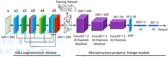
Figure 1.
Architecture of the data augmentation and microstructure–property linkage model using deep learning.
2.1. Data Augmentation Module
The data augmentation module adopted five convolution layers with diverse size filters, as shown in Table 1.

Table 1.
Network architecture of the data augmentation module.
Usually, the U-Net architecture consists of a contracting channel and an expansive channel. In the downsampling step of the U-Net architecture, the local features of the input images are extracted from different convolution layers using a convolution kernel, and the extracted local features are saved in the output channels of each convolution layer. In the upsampling step, the local features stored in each channel are synthesized to form new images after data augmentation processing. In the downsampling step, the size of the original image is continuously reduced and the number of channel is increased to extract the local features from complex images. In the upsampling step, the extracted local features are reconstructed by deconvolution and the number of channel is reduced.
Unlike the U-Net architecture, the proposed model adopts different sizes of filters (convolution kernel) in different convolution layers and maintains the size of the original image, and then reconstructs the image features extracted from each convolution layer to generate new images after data augmentation processing. The reconstructed microstructure images are comprised of grain edges and crystal grains with a diverse size, as shown in Figure 2.
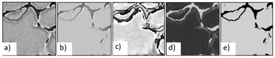
Figure 2.
Results of the data augmentation processing for micrographs images. (a) Original micrographs, (b) micrograph images extracted from convolution layer 2, (c) extracted from convolution layer 4, (d) extracted from convolution layer 5, (e) final micrograph images in black and white.
It should be mentioned that the data augmentation module using the concise and efficient convolution network structure (five convolution layers and an output channel in each convolution layer) has the obvious advantage in that it can avoid overfitting in the case of supplying a few training images, and has a higher model accuracy and computational efficiency, whereas the traditional U-Nets mainly uses 19–25 convolution and deconvolution layers and 512 channels, and several million images are needed during training the U-Nets.
2.2. Microstructure–Property Linkage Module
The micrograph images after data augmentation processing can be used as the training dataset of the microstructure–property linkage module. In this work, the microstructure–property linkage module adopted a modified VGG model to establish the relationship between the microstructure and material property, as shown in Table 2.
Table 2.
Network architecture of the microstructure–property linkage module.
3. Results and Discussion
In order to verify the prediction accuracy of the proposed data augmentation and microstructure–property model, we collected the specimens of Z3CN20-09M cast stainless steel, which were heat treated at 1030, 1080, 1130, 1180, 1230, and 1280 °C for 8 h, respectively. The 535 × 400 pixel micrographs were taken by an optical metallographic microscope for each specimen where austenite was labeled as white and ferrite as dark areas, as shown in Figure 3. The impact properties of these samples were measured by an instrumented impact tester (NI500, NCS, China) and assigned as target values of the corresponding images.
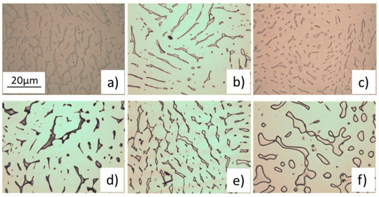
Figure 3.
Micrographs of the cast stainless steel, which were heat treated at different temperatures for 8 h (a) at 1030 °C, (b) at 1080 °C, (c) at 1130 °C, (d) at 1180 °C, (e) at 1230 °C, and (f) at 1280 °C.
3.1. Data Preparation
The dataset of 1500 samples heat treated at 1030, 1080, 1130, 1230, and 1280 °C were used to train the model and another dataset of 200 at 1180 °C was used to test the prediction results. Table 3 presents the heat treatment temperature (°C) corresponding to the micrographs and impact energies (J).
Table 3.
Heat treatment temperature (°C), micrograph images, and impact energy (J).
As seen in Table 3, ferrite is the key microstructure affecting the impact property of austenitic stainless steels [28]. The ferrite gradually grew from a reticulated, island morphology to a granular, spherical shape in the temperature range from 1030 °C to 1130 °C, and then appeared as bulk grains with the increase in the solution temperature to 1280 °C. In this process, the impact energy of the cast austenitic stainless steel increased first and then decreased.
The original micrographs were randomly cropped, flipped, and rotated to set up the training dataset and testing dataset for the data augmentation module and microstructure–property module. The volume fractions of ferrite in the sub-images were counted to ensure that the segmented sub-images still reflected the macroscopic features. The statistical results showed that the ferrite volume fractions of the sub-images were essentially the same as the original micrographs. With the above preprocessing for the original micrographs, the dataset was used for the training and testing data.
3.2. Data Augmentation Processing
To eliminate noise in the original microscope graphs, the data augmentation module was used to augment the sub-images and obtain a high quality dataset. In this work, the data augmentation model adopted five convolution layers with diverse size filters, as shown in Figure 1 and Table 1.
The data augmentation model adopted the MSELoss module in PyTorch as the loss function
where x, y are the original image and output image with an n × n pixel size. The Adam (adaptive moment estimation) module is used as an optimizer of backward. Figure 4 shows the four group output images reconstructed by the original images in different convolution layers.
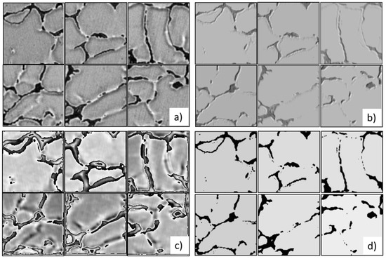
Figure 4.
Results of the data augmentation processing for six micrographs images. (a) Original micrographs, (b) micrograph images extracted from convolution layer 2, (c) extracted from convolution layer 4, and (d) final micrograph images in black and white.
As seen in Figure 4d, the ferrites (dark areas) were precisely distinguished. All sub-images reprocessed by the data augmentation module could be used as the training dataset and testing dataset for the microstructure–property module. The deep learning model using the concise network architecture has a remarkable advantage, which has fewer weight parameters and computation cost.
3.3. Microstructure–Property Linkage
In this work, we used a modified VGG model to establish the relationship between the microstructure and impact property in cast austenitic stainless steel. The modified VGG (a variant of CNN) architecture is composed of three modules: the convolutional layer, the AAP (adaptive average pooling) layer, and the nonlinearity, as shown in Figure 1. The parameters and hyper-parameters in the network architecture are given in Table 2. In the convolutional layer, three Conv2D blocks were adopted and each Conv2D block included batch normalization and ReLU activation function. The MaxPool operation was used to reduce the image size. The AAP (adaptive average pooling) layer was added after the final convolutional layer and adapted AdaptiveAvgPool2d operation in PyTorch. The dropout operation was added between FC layers by randomly dropping neurons and the corresponding parameters during model training to improve the generalization of the VGG model and prevent overfitting.
In order to provide extraordinary representational power to the modified VGG, we used the nonlinearities unit ReLU(x), which is very efficient when optimizing the parameters of an entire VGG using the gradient descent method because the gradient of ReLU(x) is always 1 when x > 0. ReLU(x) = max(x, 0) is the rectified linear unit operation on (x). Obviously, the final output is a nonlinear function of inputs in the full connection layer. In addition, we used MSELoss as the loss criterion function and the Adam module as the optimizer of backward.
Unlike the conventional VGG structure, the modified VGG model could autonomously select the best channel among 32 channels in the last Conv2D layer according to the inner product values in the Gram matrix, and then the 50 × 50 × 32 images were transformed into 10 × 10 × 1 images using APP. The simplified model had a higher model accuracy and calculation efficiency than the traditional VGG model, in which the model weight parameters were only 33% of those in the traditional VGG [22].
Figure 5 shows the feature maps of five samples extracted from different convolutional layers. It can be seen that the microstructure features were extracted from the original images with 200 × 200 pixels (Figure 5a) and reshaped into 32 feature maps with 50 × 50 × 32 pixels through three Conv2D blocks (in Figure 5b, only one of 32 feature maps is given), then the best channel was selected and reshaped into the feature map with 10 × 10 × 1 pixels (Figure 5c) through the APP layer and the feature maps in black and white (Figure 5d) using the threshold processing. Notably, the feature maps extracted in the different layers retained important features with original microstructure images such as the ferrite area size and morphology.
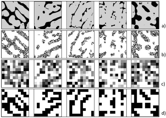
Figure 5.
Feature maps of five samples extracted from different convolutional layers. (a) Original images with 200 × 200 pixels; (b) feature maps with 50 × 50 × 32 pixels through three Conv2D blocks; (c) feature maps with 10 × 10 × 1 pixels through APP; and (d) feature maps in black and white.
To improve the prediction accuracy of the model, we adopted a novel method where the best feature vector among 32 channels can be selected according to the Gram matrix before the AAP layer, instead of the GAP (global average pooling) of 32 channels in the traditional VGG. GAP operation is usually used to obtain the global average pooling value of the feature map extracted from each channel, that is, 50 × 50 × 32 feature maps are reduced into 1 × 1 × 32 units, but the microstructure morphology information in the feature maps will fully disappear if using global average pooling for a feature map with 50 × 50 pixels.
The Gram matrix is defined as a matrix composed of the inner product of two feature vectors among 32 channels:
where X is a matrix composed of 32 feature vectors; x is a feature vector (flattened feature maps) in matrix X. The Gram matrix can reveal some intrinsic relationships between the two feature vectors. In the style transfer model [29], the Gram matrix is usually used to measure the difference between two images, and the optimization goal of the style transfer model is to minimize the difference and make the trained image continuously close to the target image. The VGG model can extract feature maps of the input images from different channels in each convolution layer. If the differences between the extracted feature images and input images are small, their inner products will become large, which means that the feature maps extracted from the two channels are similar.
Taking three samples, the feature maps of the first eight channels extracted from the last Conv2D block and their Gram matrix values are given in Figure 6. It can be seen that many feature maps in different channels were similar, for example, the feature maps in channel 1 and channels 3, 5, 6 7, 8. From Figure 6, it can also be seen that G1,1 had the maximum value among all eight feature map pairs and those feature maps were consistent with the original microscope images. Due to the extracted feature maps, the interrelation distribution rule of morphology in the original microstructure images can describe the best feature map among all channels that should perfectly retain the basic characteristics of the original image, and has the least error loss with the original image during model training. Hence, we selected the feature map extracted from the best channel as the input of the AAP pooling layer.
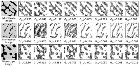
Figure 6.
Feature maps of the first eight channels extracted from the last Conv2D block and their Gram matrix values. The left images are microscope images of the samples, the right images are the corresponding feature maps with 50 × 50 pixels in different channels through three Conv2D blocks.
3.4. Predicted Results of Microstructure–Property Model
The 1500 dataset of five group samples heat treated at 1030, 1080, 1130, 1230, and 1280 °C were used to train the model and 200 datasets at 1180 °C were used to test the prediction results. Leave-one-out cross-validation was used to evaluate the generalization performance of the trained VGG. First, images generated from one of the five training datasets were removed. Then, the validation data were collected from the held-out dataset, while the training and validation data were collected from the remaining dataset. After recording the regression results estimated by the validation dataset, the removed training dataset was changed, and the same procedure was repeated until all five group samples were tested. All VGG optimizations were carried out using stochastic gradient descent (SGD) with a mini-batch size of 20 and the Adam algorithm, the objective function in which was the mean squared error between the measured impact energies and predicted values. Adam is a type of adaptive SGD algorithm.
The distributions of the prediction results obtained by the modified VGG are shown in Figure 7a. These distributions are almost Gaussian. In Figure 7b,c, only the medians of these distributions are plotted. By comparing Figure 7b with the corresponding results obtained by conventional VGG in Figure 7c, it can verify that the modified VGG can predict the impact energies more accurately from the raw micrograph images compared to the conventional VGG. This indicates that using several micrographs without any artificial image processing, the modified VGG can be well-trained, and its performance exceeds that of the conventional scheme.
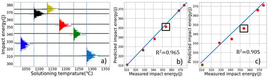
Figure 7.
The results obtained by the 1500 leave-one-out cross-validation data are shown in (a) by the violin plot. The dotted lines in (a) indicate the medians. Only the medians with modified VGG and conventional VGG are plotted in (b,c). Coefficients of determination (R2) are written in (b,c).
The predicted medians of the training dataset for the five group samples were compared with the measured impact energies, where it can be found that the modified VGG model was more accurate than the classical VGG model. The coefficient R2 of the modified VGG model was 0.965 and the medians only showed a ±2 J difference with the measured values.
To further verify the generalization performance of the models, the testing dataset of the sample at the 1180 °C solution temperature was also predicted, as shown in Figure 7b,c, which is marked in the black rectangle. The median of the predicted results using the modified VGG was 351.9 J, only 2 J different to the measured impact energy, whereas the median difference using the classical VGG was 9.1 J. Apparently, the prediction results using the modified VGG are more accurate compared with the classical VGG. This is because the impact property for the austenitic stainless steel is not only influenced by the volume fraction of ferrite, but also by other microstructure features such as the morphology and distribution of ferrite. The above results show that the modified VGG can extract the information of volume fraction and the morphology distribution of ferrite. Hence, it has superior generalization ability and can accurately predict the impact energy for the new sample.
4. Conclusions
In this work, we proposed a new model based on deep learning to improve the power of the micrograph data augmentation and constructed a microstructure–property linkage for cast austenitic steels. The main advantage compared with the conventional microstructure–property linkage models is that the model could precisely extract the microstructure features from original irregular micrographs and successfully established the relationship between the microstructure and material property. The results showed that the developed model had a higher prediction accuracy, the coefficient R2 of the model reached 0.965, and the medians were only ±2 J different to the measured impact toughness. Notably, we demonstrated that only six micrographs of the cast austenitic steel supplied sufficient information in training the deep learning model, which could be widely applied in the discovery of novel materials.
The present study is not limited to the case of irregular micrographs for cast austenitic steels, but can also be applied to any other material. In addition, we used only one property for each micrograph, namely, impact toughness, but various properties such as yield strength, elongation, etc., can be used simultaneously as output targets. It is only necessary to adjust the output of the VGG from one to multiple.
Author Contributions
G.X. conceived the idea, developed the model and wrote the paper; X.Z. and J.X. participated in the paper writing and discussion. All authors have read and agreed to the published version of the manuscript.
Funding
This work was financially supported by the National Natural Science Foundation of China (No. 52175284) and the State Key Lab of Advanced Metals and Materials in University of Science and Technology Beijing (No. 2021-ZD08).
Institutional Review Board Statement
This study did not involve humans or animals.
Informed Consent Statement
This study did not involve humans or animals.
Data Availability Statement
The data that support the findings of this study are available from the corresponding author, Gang Xu (email: watermoon2012@gmail.com), upon reasonable request.
Acknowledgments
This work was also financially supported by the Fundamental Research Funds for the Central Universities (No. FRF-TP-19-007A1).
Conflicts of Interest
The authors declare that they have no known competing financial interests or personal relationships that could have appeared to influence the work reported in this paper.
References
- Rajan, K. Materials Informatics: The Materials “Gene” and Big Data. Annu. Rev. Mater. Res. 2015, 45, 153. [Google Scholar] [CrossRef]
- Ge, M.; Su, F.; Zhao, Z.; Su, D. Deep learning analysis on microscopic imaging in materials science. Mater. Today Nano 2020, 11, 100087. [Google Scholar] [CrossRef]
- Konda, N.; Verma, R.; Jayaganthan, R. Machine Learning based predictions of fatigue crack growth rate of additively manufactured Ti6Al4V. Metals 2022, 12, 50. [Google Scholar] [CrossRef]
- Honysz, R. Modeling the Chemical Composition of Ferritic Stainless Steels with the Use of Artificial Neural Networks. Metals 2021, 11, 724. [Google Scholar] [CrossRef]
- Choi, W.; Won, S.; Kim, G.-S.; Kang, N. Artificial Neural NetworkModelling of the Effect of Vanadium Addition on the Tensile Properties and Microstructure of High-Strength Tempcore Rebars. Materials 2022, 15, 3781. [Google Scholar] [CrossRef] [PubMed]
- Churyumov, A.; Kazakova, A.; Churyumova, T. Modelling of the Steel High-Temperature Deformation Behaviour Using Artificial Neural Network. Metals 2022, 12, 447. [Google Scholar] [CrossRef]
- Chen, S.; Kaufmann, T. Development of data-driven machine learning models for the prediction of casting surface defects. Metals 2022, 12, 1. [Google Scholar] [CrossRef]
- Wang, C.S.; Fu, H.D.; Jiang, L.; Xue, D.Z.; Xie, J.X. A property-oriented design strategy for high performance copper alloys via machine learning. npj Comput. Mater. 2019, 5, 87. [Google Scholar] [CrossRef]
- Wu, Y.J.; Fang, L.; Xu, Y.B. Predicting interfacial thermal resistance by machine learning. npj Comput. Mater. 2019, 5, 56. [Google Scholar] [CrossRef]
- Ward, L.; O’Keeffe, S.C.; Stevick, J.; Jelbert, G.R.; Aykol, M.; Wolverton, C. A machine learning approach for engineering bulk metallic glass alloys. Acta Mater. 2018, 159, 102. [Google Scholar] [CrossRef]
- Shin, D.; Yamamoto, Y.; Brady, M.P.; Lee, S.; Haynes, J.A. Modern data analytics approach to predict creep of high-temperature alloys. Acta Mater. 2019, 168, 321. [Google Scholar] [CrossRef]
- Yabansu, Y.C.; Steinmetz, P.; Hötzer, J.; Kalidindi, S.R.; Nestler, B. Extraction of reduced-order process-structure linkages from phase-field simulations. Acta Mater. 2017, 124, 182–194. [Google Scholar] [CrossRef]
- Yucel, B.; Yucel, S.; Ray, A.; Duprez, L.; Kalidindi, S.R. Mining the correlations between optical micrographs and mechanical properties of cold-rolled HSLA steels using machine learning approaches. Integr. Mater. Manuf. Innov. 2020, 9, 240–256. [Google Scholar] [CrossRef]
- Khatavkar, N.; Swetlana, S.; Singh, A.K. Accelerated prediction of Vickers hardness of Co- and Ni-based superalloys from microstructure and composition using advanced image processing techniques and machine learning. Acta Mater. 2020, 196, 295–303. [Google Scholar] [CrossRef]
- Fan, Y.; Yang, X.; Shi, D.; Tan, L.; Huang, W. Quantitative mapping of service process-microstructural degradation-property deterioration for a Ni-based superalloy based on chord length distribution imaging process. Mater. Des. 2021, 203, 109561. [Google Scholar] [CrossRef]
- Paulson, N.H.; Priddy, M.W.; McDowell, D.L.; Kalidindi, S.R. Reduced-order structure-property linkages for polycrystalline microstructures based on 2-point statistics. Acta Mater. 2017, 129, 428. [Google Scholar] [CrossRef]
- Fernandez-Zelaia, P.; Joseph, V.; Kalidindi, S.R.; Melkote, S.N. Estimating mechanical properties from spherical indentation using Bayesian approaches. Mater. Des. 2018, 147, 92. [Google Scholar] [CrossRef]
- Hart, G.L.W.; Mueller, T.; Toher, C.; Curtarolo, S. Machine learning for alloys. Nat. Rev. Mater. 2021, 6, 730. [Google Scholar] [CrossRef]
- Morgan, D.; Jacobs, R. Opportunities and challenges for machine learning in materials science. Annu. Rev. Mater. Res. 2020, 50, 71. [Google Scholar] [CrossRef]
- Thankachan, T.; Prakash, K.S.; Pleass, C.D.; Rammasamy, D.; Prabakaran, B.; Jothi, S. Artificial neural network to predict the degraded mechanical properties of metallic materials due to the presence of hydrogen. Int. J. Hydrogen Energy 2017, 42, 28612. [Google Scholar] [CrossRef]
- Feng, S.; Zhou, H.; Dong, H. Using deep neural network with small dataset to predict material defects. Mater. Des. 2019, 162, 300–310. [Google Scholar] [CrossRef]
- Kondo, R.; Yamakawa, S.; Masuoka, Y.; Tajima, S.; Asahi, R. Microstructure recognition using convolutional neural networks for prediction of ionic conductivity in ceramics. Acta Mater. 2017, 141, 29–38. [Google Scholar] [CrossRef]
- Cecena, A.; Daia, H.; Yabansub, C.Y.C.; Kalidindia, S.R.; Song, L. Material structure-property linkages using three-dimensional convolutional neural networks. Acta Mater. 2017, 11, 53. [Google Scholar] [CrossRef]
- Nouira, A.; Crivello, J.C.; Sokolovska, N. Crystal GAN: Learning to discover crystallographic structures with generative adversarial networks. arXiv 2019, arXiv:1810.11203. [Google Scholar]
- Xie, T.; Grossman, J.C. Hierarchical visualization of materials space with graph convolutional neural networks. J. Chem. Phys. 2018, 149, 174111. [Google Scholar] [CrossRef]
- Chen, C.; Ye, W.; Zuo, Y.; Zheng, C.; Ong, S.P. Graph networks as a universal machine learning framework for molecules and crystals. Chem. Mater. 2019, 31, 3564. [Google Scholar] [CrossRef]
- Wang, C.; Shi, D.; Li, S. A study on establishing a microstructure-related hardness model with precipitate segmentation using deep learning method. Materials 2020, 13, 1256. [Google Scholar] [CrossRef]
- Reiter, J.; Bernhard, C.; Presslinger, H. Austenite grain size in the continuous casting process: Metallographic methods and evaluation. Mater. Charact. 2008, 59, 737–746. [Google Scholar] [CrossRef]
- Gatys, L.; Ecker, A.S.; Bethge, M. Image Style Transfer Using Convolutional Neural Networks. In Proceedings of the IEEE Conference on Computer Vision and Pattern Recognition (CVPR), Las Vegas, NV, USA, 27–30 June 2016; pp. 2414–2423. [Google Scholar]


Disclaimer/Publisher’s Note: The statements, opinions and data contained in all publications are solely those of the individual author(s) and contributor(s) and not of MDPI and/or the editor(s). MDPI and/or the editor(s) disclaim responsibility for any injury to people or property resulting from any ideas, methods, instructions or products referred to in the content. |
© 2023 by the authors. Licensee MDPI, Basel, Switzerland. This article is an open access article distributed under the terms and conditions of the Creative Commons Attribution (CC BY) license (https://creativecommons.org/licenses/by/4.0/).