Abstract
Laser cleaning is a good alternative to ablate and remove contaminants from different samples. To meet the practical demand, we present the elemental analysis of Q235 steel samples, using laser-induced breakdown spectroscopy (LIBS) to enhance the laser cleaning process. Two samples were selected and kept in water and soil for 4 and 7 days, respectively. Half of the samples were then cleaned using the laser cleaning method. The objectives were to promote the application of laser cleaning, generalize the LIBS for the laser cleaning settings, and identify the different sources of contaminations. Numerous elements were determined by analyzing the LIBS spectra, including Fe, Mn, Cu, Si, Ni, Cr, C, S, and P. After 20 excitation cycles, LIBS signals were comparatively stable and could participate in the ensuing classification modeling procedure. The contaminated samples were noticeably stronger overall than the uncontaminated samples, with the higher the concentration of a certain element, the higher the characteristic spectral intensity of LIBS. The typical spectral intensity and concentration of the two samples were found to be in good agreement.
1. Introduction
Steel is the most important material used in numerous industrial domains, and it may be transformed into a variety of alloys with distinct properties to satisfy a range of industrial requirements. In 2021, 1951 million tons of crude steel were consumed globally, and the average growth rate for the previous five years was 3.8% [1]. Although iron is the primary component of steel, minor and trace elements play a major role in the steel’s unique qualities, including toughness, strength, hardness, and corrosion resistance [2,3,4]. Non-metal elements like carbon, nitrogen, phosphorus, and sulfur, and metal elements like manganese, chromium, nickel, molybdenum, and vanadium can be used to categorize these elements [5]. Among the latter, manganese is a powerful deoxidizer and desulfurizer in steel, improving steel’s quench capacity and workability [6]. In contrast, chromium can significantly improve the strength, hardness, oxidation resistance, corrosion resistance, and wear resistance of steel [7]. Rapid identification of steel and precise determination of the minor and trace metal element concentrations in steel are the essential stages in the recycling and reuse of steel waste, in order to conserve steel resources and guarantee product quality.
Currently, there are several steel metal element analysis techniques which include X-ray fluorescence (XRF), particularly energy-dispersed X-ray fluorescence (EDXRF) [8,9,10,11,12], spark optical emission spectroscopy [13], inductively coupled plasma atomic emission spectrometry (ICP-AES) [14,15], inductively coupled plasma mass spectrometry (ICP-MS) [16,17,18,19], isotope dilution spark source mass spectrometry (ID-SSMS) [20], and flame atomic absorption spectrometry (FAAS) [21,22]. However, these traditional analytical methods need complex and time-consuming sample preparations; therefore, a more practical, accurate, and rapid classification approach for steel is required. LIBS offers a number of specific features, including direct analysis of materials, possibly at a remote distance, fast analyzing speed, multi-element analysis capability, and microdamage detection, without the materials being pretreated through a complex preparation procedure. Such characteristics are vital for a variety of applications, particularly industrial process control, where conventional analytical methods face significant challenges. LIBS is an atomic emission spectroscopy technique that utilizes a laser pulse to create a plasma, with the emission lines from the plasma used to determine the composition of samples [23,24]. Recent years have seen a lot of work put into LIBS analysis at high temperatures [25]. The comparison of plasma characteristics between room temperature and high temperature [26], including plasma temperature, electron density, and spectral intensity, has been the subject of numerous studies aimed at improving the detection system [27,28]. Hermann et al. evaluated the pressure and observed the evidence of blackbody radiation from a laser-induced plasma, and demonstrated the local thermodynamic equilibrium through the equality between blackbody temperature and excitation temperature of atoms and ions, by simulating the plasma emission spectra [29,30,31,32].
The main emphasis of research on high-temperature quantitative LIBS analysis is how to create a calibration model. Carlhoff et al. [33] and Aragón et al. [34] first realized LIBS for the in-situ analysis of molten steel. Calibration curves have often been built using linear or quadratic fitting. Sun et al. [35] and Noll et al. [36] used samples heated to a high temperature with a predetermined amount of source materials to produce various elemental concentrations for calibration curves. Peter et al. [37] established calibration curves for Cr, Ni, C, P, and S of steel melts in the vacuum ultraviolet region. Seven separate molten Al alloy samples were used by Rai et al. [38] to create ratio calibration curves for Cr, Mg, and Zn, using Fe as the reference element. Sturm et al. [39] developed calibration curves using univariate regression of the mass fraction ratios in liquid slags with the mean of the spectral line ratios (ratio of the peak area of the analyte line and reference line). Sun et al. [40] used a partial least squares (PLS) regression model to construct the calibration curves for Si, Mn, Cr, Ni, and V in eight molten steel samples, utilizing six samples for calibration and the other two for testing. Ma and Cui modified the PLS regression model and used the initial 200 spectra for calibration and the final 100 spectra for testing to construct the calibration curves for Si and Mn in ten standard samples [41]. With the help of stand-off LIBS, Delgado et al. [42] developed distinction strategies based on discriminant function analysis for particular steel grades at elevated temperatures. Hermann et al. employed the calibration-free LIBS approach to study the two-step procedure for trace element analysis in food [43], multi-elemental analysis of thin film [44], and quantification of surface contamination on optical glass [45].
The study aims to control and enhance the laser cleaning process of the contaminated samples and identify the sources of different contaminants using the LIBS technique. This study adopted laser cleaning to remove the contaminations from the locally prepared Q235 steel samples (contaminated with soil and water). Laser cleaning has been considered a high-efficiency and environmentally-friendly cleaning technology, a promising method to remove contaminants, including oil, paint, and oxide layers [46]. LIBS was used to investigate the elemental analysis in the contaminated and laser-cleaned samples. To ensure the consistency of the spectrum and plasma intensity, the related plasma map was also captured at the same time as the LIBS spectrum detection. It has been proven that the excitation times have an impact on the spectrum intensity of the LIBS elemental properties. The aim was to generalize the LIBS for the laser cleaning parameters, identify the sources of different contamination, and promote the applications of laser cleaning in this field. Different elements were found, for example, Fe, Mn, Cu, Si, Ni, Cr, C, S, and P, by analyzing the LIBS spectra. Only 2 samples, however, were examined; hence, additional testing of multiple sample modeling is needed to conduct quantitative and qualitative analysis.
2. Materials and Methods
2.1. Sample Preparation
Our test samples were two Q235 alloy steel samples. Both the samples were half contaminated and half laser-cleaned. Sample 1 was contaminated with tap water (for 4 days), and sample 2 was contaminated with soil (for 7 days with 4–5 cm depth), in Jinan City, Shandong Province, China. The samples and their location are shown in Figure 1. Q235, a simple carbon structural steel, is extensively used in China. It is utilized in production without heat treatment, since it is mild steel and has good plasticity and weldability. The Q denotes the yield point, and the 235 indicates the yield strength.
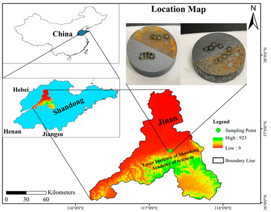
Figure 1.
Map illustrating the sampling site location in this study. The inset shows sample 1 (left, half-contaminated with tap water and half-laser-cleaned), and sample 2 (right, half-contaminated with soil and half-laser-cleaned).
2.2. Experimental Setup
The available homemade laser cleaning setup (with 350 W power, 30 mJ single pulsed energy, and spot size 0.7 mm, Laser Institute of Shandong Academy of Sciences, Jinan, China) mainly consisted of a laser system, optical fibers, and a monitory system (see Table 1). The monitory system (computer) integrated laser, power supply, water cooling, control system, and other unit components. The laser output beam was hand-held and had the functions of cleaning and dust collection. The control software was also homemade and had two operating modes: professional and simple, which was suitable for operators.

Table 1.
Parameter of the laser cleaning system.
Figure 2 depicts the experimental configuration utilized to get the LIBS spectra [47]. A Q-switched Nd: YAG laser (Q-smart 450, Quantel, Cournon-d’Auvergne, France) was used to produce the laser beam, which had a wavelength of 1064 nm, a pulse duration of 6 ns, and an 8 Hz pulse repetition rate. The laser energy and delay time were optimized to be 50 mJ per pulse and 1.28 μs, respectively. A quartz lens with a 100 mm focal length was employed to focus the laser beam on the sample’s surface. In order to collect the laser-induced plasma light, a 10 mm focal length lens with a diameter of 10 mm, transmitted with the help of an optical fiber to a 5-channel spectrograph, coupled with a charge-coupled device (CCD) (AvaSpec-ULS2048-5-USB2, Avantes, Apeldoorn, The Netherlands), was employed. The spectral range of the 5-channel spectrometer was 185–669 nm, with the resolution ranging from 0.033 nm to 0.060 nm for different channels. During the measurement, each point was excited 40 times, and the spectral data were recorded. Additionally, a three-dimensional platform was used to regulate the scanning of the test positions, and laser-ranging equipment was used to precisely control the focusing position. To avoid contaminating the optical system or obstructing the laser beam, we employed vacuum cleaners to collect the sample powder, generated near the surface of the sample, during the experiment. The traced elements in the two samples are shown in Table 2.
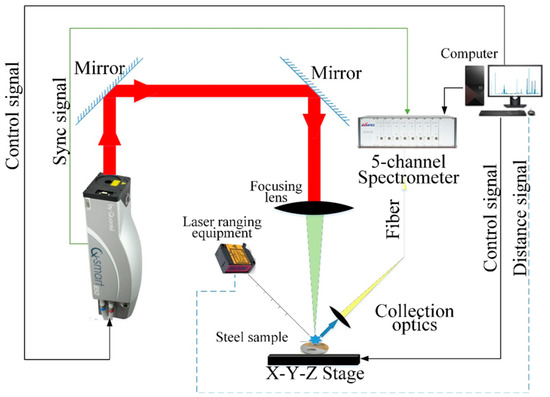
Figure 2.
Schematic diagram of LIBS system.
Table 2.
Trace elements content of the two Q235 steel samples.
3. Results and Discussion
3.1. LIBS Spectra
The purpose of the study was to improve and control the laser cleaning of contaminated samples and to use the LIBS approach to identify the sources of various impurities. The Q235 steel samples used in this study were locally prepared, and the contamination was removed using laser cleaning. Firstly, we analyzed the whole spectrum and the characteristic spectral lines of a single element. Then, the difference in LIBS spectrum between the contaminated and laser-cleaned samples was studied, as shown in Figure 3 and Figure 4. The spectra contained information about the concentrations of all naturally-occurring elements in the samples. Compared with those in the NIST atomic spectra database, Fe, Mn, Cu, Si, Ni, Cr, C, S, and P were observed in the LIBS spectra [48]. Figure 4 demonstrates the single-element spectral line analysis by taking the mean values of the 20th to 40th excitation spectra. Finally, the characteristic spectrum of each element was modeled by support vector machine (SVM) classification [49]. The samples were divided into a training set and a test set. The training set was used for training, and the training model was used to predict the data in the test set.
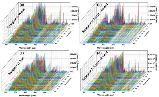
Figure 3.
LIBS spectra (40 excitations), (a) Sample 1: contaminated with water, (b) Sample 1: laser-cleaned, (c) Sample 2: contaminated with soil, and (d) Sample 2: laser-cleaned.
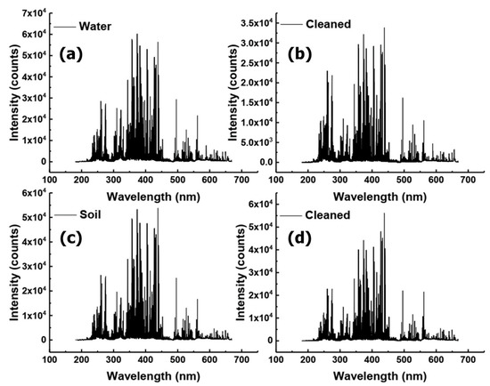
Figure 4.
Single element spectral line analysis. (a) Contaminated with water, (b) laser-cleaned, (c) contaminated with soil, and (d) laser-cleaned. (Mean values of the 20th to 40th excitation spectra).
The plasmas from the images were also be preliminarily analyzed, as shown in Figure 5. Under the same laser excitation energy, the LIBS plasma intensities of the contaminated samples were stronger than that of the cleaned samples. This result corresponds to the spectral outcome [50]. We analyzed the LIBS spectra after 20 excitations because the laser action removes the oxide layer’s surface after 20 excitations, and this is because the effect of excitation times from prior experiments played a particular role in laser cleaning. LIBS signals after 20 excitations are relatively stable and can participate in the subsequent classification modeling process. In terms of overall strength, the contaminated steel sample was significantly greater than the uncontaminated one. At the same time, the LIBS spectral intensity of the steel samples cleaned by laser was between the uncontaminated and contaminated ones.
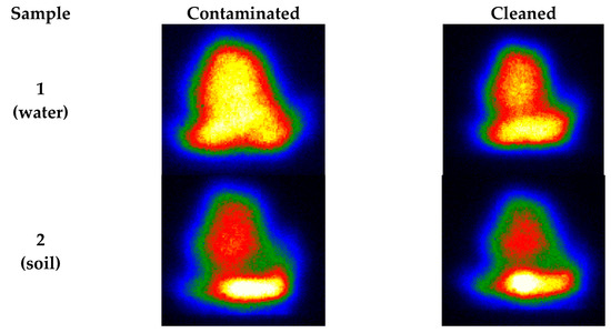
Figure 5.
Plasma images correspond to different samples (first excitation).
The signal intensity with respect to the number of laser shots is given in Figure 6. We analyzed a single characteristic line of one particular element. The spectral intensities of contaminated samples and laser-cleaned samples were compared with each other. The spectral lines of Fe-234.36 nm, Fe-248.30 nm, C-193.03 nm, Cr-425.45 nm, Cu-213.57 nm, Mn-403.04 nm, Ni-300.25 nm, and Si-288.10 nm were selected for analysis (see Reference [12] and the references therein). The reason why the characteristic spectral lines of P and S were not selected was that the content of P and S was low, resulting in no obvious comparison of results. It could be clearly seen from the comparison curve that the characteristic spectral intensities of Si, Mn, C, and Cr elements had the same rules. For the same sample, the LIBS characteristic spectrum intensity of the contaminated samples was larger than that of the laser-cleaned samples. After data analysis, Fe, Cu, and Ni were shown to have similar rules, which were not as obvious as the first four elements. The intensity of the characteristic spectrum from a single element also corresponded to the element concentration. There was good correspondence between the characteristic spectral intensity and concentration of the two samples. Also, the LIBS spectral intensity of the sample with higher concentration was higher.
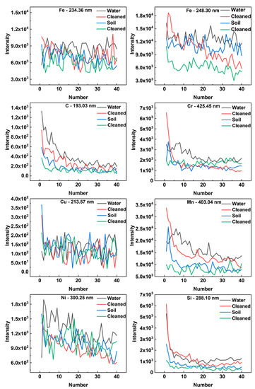
Figure 6.
The signal intensity vs. the number of laser shots.
3.2. Analysis and Methods
Spectral background removal and normalization: As a result of the instability of the plasma and the matrix effect in LIBS, standardization and normalization of the spectral data were crucial pre-treatment processes for the original spectra. The environment’s spectral background and the removal of the laser’s lamp pump can be expressed as follows:
where I is the spectral intensity with the background of the environment and the laser’s lamp pump removed, Iraw is the raw spectral intensity, and Ibackground represents the measured spectral intensity when only the laser pump light is turned on. Normalization is realized using the following equation:
where Imapminmax expresses the corresponding normalized value, and Imax and Imin are the maximum and minimum spectral intensities for each channel of the spectrometer with the removed background, respectively. Due to the independence of the spectrometer’s 5 channels, the normalization of the spectrum was processed separately in this study according to various channels. The corresponding typical spectra are shown in Figure 3. The necessary components must be extracted from the spectral information as independent variables for subsequent modeling after the spectrum has been pre-treated and standardized.
Support Vector Machine: SVM is a generalized linear classifier that uses a maximum-margin hyperplane that is obtained by training the samples for binary classification. SVM is typically applied to regression analysis, classification, and pattern recognition [51]. The following is the key tenet of SVM: the training set is {(xi,yi), i = 1,2,3…,N}, where xi ∈ RD is the input variable and yi ∈ {−1,1} is the predicted output. SVM can determine the optimal hyperplane (ω × x) + b = 0 between two types of data, where b is the distance from the plane to the origin, and ω is the normal phase vector of the plane. The classifier in the case of linear separability is:
SVM maps data from low- and high-dimensional spaces in the case of linear inseparability; therefore, the classifier becomes:
where sgn{} represents the sign function, ai is the Lagrangian multiplier, xi is the value of the training sample, x is the sample label to be classified, and K (xi × x) is the kernel function. In this study, a Gaussian radial basis function is used to establish the models, and a genetic algorithm is utilized to optimize the penalty parameter c and kernel parameter g [52].
Wavelength selection for elements in the LIBS spectrum: The spectral lines of each element were obtained by comparing the peak position in the LIBS spectrum with the corresponding wavelength of the elements in the NIST database [48]. The specific wavelengths are shown in Table 3. The independent variables were first chosen to be the spectral intensities of the spectral pixels that corresponded to these wavelengths.
Table 3.
Corresponding specific wavelengths of the samples.
Matrix effect reduced: In LIBS spectra, matrix effects resulting from the physical and chemical properties of elements are ubiquitous. The spectral intensity of the chosen wavelength is decreased from its peak value by the minimum spectral line intensity of the first 25 and last 25 pixels, in order to lessen the matrix effect that affects the quantitative analysis. First, the spectral intensities of the 25 front and rear pixels, as well as the pixel’s wavelength-corresponding spectral intensity, were obtained. By subtracting the spectral intensities of the pixels from the minimum value of the intensity of the 25 pixels before and after them, the modified characteristic spectral intensities were subsequently obtained. The equation reads as follows:
where is the corrected spectral intensity, is the original spectral intensity, i is the number of pixels corresponding to the characteristic wavelength of the selected element, and j is the number of pixels in the spectral waveform.
Lorentz fitting of selected spectral peaks: The Lorentz fitting method can be used to process each peak, and the corrected peak value can be utilized as the independent variable. The curve of the corresponding element in the LIBS spectrum is approximately similar to the Lorentz curve. Every distinctive line was handled the same way. Spectral normalization and pre-processing were followed by the acquisition of independent variables for later SVM modeling. Both samples’ categorization accuracy after SVM classification was 100%.
The overall strength of the contaminated samples was substantially higher than the strength of the uncontaminated samples, and the characteristic spectral intensity of LIBS increased with increasing elemental concentration. It was found that the typical spectral intensity and concentration of the samples were found to be in good agreement. However, as only 2 samples were tested, multiple sample modeling has to be investigated further for both quantitative and qualitative analysis, with LIBS integrated with a laser cleaning system for real-time monitoring. Overall, obtaining the ideal laser cleaning settings through online monitoring might not only lower energy costs but also guarantee the quality of the cleaned surface.
4. Conclusions
Based on the LIBS approach to pinpoint the origin of various pollutants, this study was designed to enhance the efficacy of laser-cleaned samples. First, laser cleaning was employed to remove the contaminations from the locally prepared Q235 steel samples (contaminated with soil and water). Then the elemental analysis of the contaminated and laser-cleaned samples was examined using LIBS. Many elements, including Fe, Mn, Cu, Si, Ni, Cr, C, S, and P, were found by examining the LIBS spectra. It was confirmed that the excitation times affect the spectrum intensity of the LIBS elemental characteristics. The corresponding plasma map was also recorded at the same time as LIBS spectrum detection, to verify the consistency of the spectrum and plasma intensity. For a deep understanding of the origin of the contaminants and to perform quantitative and qualitative analysis, multiple samples should be selected. Of particular interest in the study, it is believed that this study will open new advances for the laser cleaning community.
Author Contributions
Conceptualization, S.Z.U.D. and W.Z.; methodology, S.Z.U.D. and W.Z.; software, S.Z.U.D., C.S. and W.Z.; validation, S.Z.U.D. and W.Z.; formal analysis, S.Z.U.D., C.S. and W.Z.; investigation, S.Z.U.D.; resources, S.Z.U.D., Q.Z., Y.W. and W.Z.; data curation, S.Z.U.D. and W.Z.; writing—original draft preparation, S.Z.U.D.; writing—review and editing, S.Z.U.D. and W.Z.; visualization, S.Z.U.D.; supervision, W.Z.; project administration, Q.Z. and Y.W.; funding acquisition, Q.Z. and Y.W. All authors have read and agreed to the published version of the manuscript.
Funding
This work is supported by the National Key Research and Development Program of China (Grant No. 2021YFB3201905), Natural Science Foundation of Shandong Province (Grant Nos. ZR2022QF083, ZR2022QF035), The Major Scientific and Technological Innovation Project of Shandong Province (Grant No. ZR2020KC012), and National Innovation and Entrepreneurship Training Program for college students (Grant No. 202210431012). Zaheer Ud Din also acknowledges the support of the Young Doctors Cooperation Fund, Qilu University of Technology (Shandong Academy of Sciences) (Grant No. 2019BSHZ006) and Undergraduate Climbing Project, International School for Optoelectronic Engineering, Laser Institute, Qilu University of Technology (Shandong Academy of Sciences) (Grant No. GDPD202011).
Data Availability Statement
Not applicable.
Conflicts of Interest
The authors declare no conflict of interest.
References
- World Steel in Figures. Available online: https://worldsteel.org/wp-content/uploads/World-Steel-in-Figures-2022.pdf (accessed on 7 June 2022).
- Wada, T.; Hagel, W.C. Effect of trace elements, molybdenum, and intercritical heat treatment on temper embrittlement of 2-1/4Cr-1 Mo steel. Metall. Trans. A 1976, 7, 1419–1426. [Google Scholar] [CrossRef]
- Swindeman, R.; Sikka, V.; Klueh, R. Residual and trace element effects on the high-temperature creep strength of austenitic stainless steels. Metall. Trans. A 1983, 14, 581–593. [Google Scholar] [CrossRef]
- Melford, D. The influence of residual and trace elements on hot shortness and high temperature embrittlement. Philos. Trans. R Soc. Lond. A 1980, 295, 89–103. [Google Scholar] [CrossRef]
- Zhang, Y.; Sun, C.; Gao, L.; Yue, Z.; Shabbir, S.; Xu, W.; Wu, M.; Yu, J. Determination of minor metal elements in steel using laser-induced breakdown spectroscopy combined with machine learning algorithms. Spectrochim. Acta Part B At. Spectrosc. 2020, 166, 105802. [Google Scholar] [CrossRef]
- Brook, R.; Da Silva, P.S.P. The influence of manganese on the fracture toughness of nickel steels. Int. J. Fract. 1976, 12, 27–32. [Google Scholar] [CrossRef]
- Maslyuk, V.A.; Lvova, G.G.; Kurovskii, V.Y.; Mamonova, A.A. Effect of chromium and manganese nitrides on the structure and properties of Kh18N15 powder stainless steel. Powder Metall. Met. Ceram. 2011, 50, 289. [Google Scholar] [CrossRef]
- Tiwari, M.K.; Singh, A.K.; Sawhney, K.J.S. Analysis of stainless steel samples by energy dispersive X-ray fluorescence (EDXRF) spectrometry. Bull. Mater. Sci. 2001, 24, 633–638. [Google Scholar] [CrossRef]
- Nagoshi, M.; Aoyama, T.; Tanaka, Y.; Ishida, T.; Kinoshiro, S.; Kobayashi, K. Quantitative Analysis of Nb in Steel Utilizing XRF-yield XAFS Edge Jump. ISIJ Int. 2013, 53, 2197–2200. [Google Scholar] [CrossRef]
- Bosco, G.L. Development and application of portable, hand-held X-ray fluorescence spectrometers. TrAC Trends Anal. Chem. 2013, 45, 121–134. [Google Scholar] [CrossRef]
- Volkov, A.I.; Alov, N.V. Method for improving the accuracy of continuous X-ray fluorescence analysis of iron ore mixtures. J. Anal. Chem. 2010, 65, 732–738. [Google Scholar] [CrossRef]
- Wang, Z.; Deguchi, Y.; Shiou, F.; Yan, J.; Liu, J. Application of laser-induced breakdown spectroscopy to real-time elemental monitoring of iron and steel making processes. ISIJ Int. 2016, 56, 423–435. [Google Scholar] [CrossRef]
- Hemmerlin, M.; Meilland, R.; Falk, H.; Wintjens, P.; Paulard, L. Application of vacuum ultraviolet laser-induced breakdown spectrometry for steel analysis—Comparison with spark-optical emission spectrometry figures of merit. Spectrochim. Acta Part B At. Spectrosc. 2001, 56, 661–669. [Google Scholar] [CrossRef]
- Kataoka, H.; Okamoto, Y.; Matsushita, T.; Tsukahara, S.; Fujiwara, T.; Wagatsuma, K. Magnetic drop-in tungsten boat furnace vaporisation inductively coupled plasma atomic emission spectrometry (MDI-TBF-ICP-AES) for the direct solid sampling of iron and steel. J. Anal. Atomic Spectrom. 2008, 23, 1108–1111. [Google Scholar] [CrossRef]
- Wiltsche, H.; Brenner, I.B.; Prattes, K.; Knapp, G. Characterization of a multimode sample introduction system (MSIS) for multielement analysis of trace elements in high alloy steels and nickel alloys using axially viewed hydride generation ICP-AES. J. Anal. Atomic Spectrom. 2008, 23, 1253–1262. [Google Scholar] [CrossRef]
- Yasuhara, H.; Okano, T.; Matsumura, Y. Determination of trace elements in steel by laser ablation inductively coupled plasma mass spectrometry. Analyst 1992, 117, 395–399. [Google Scholar] [CrossRef]
- Okano, G.; Igarashi, S.; Ohno, O.; Yamamoto, Y.; Saito, S.; Oka, Y. Determination of trace amounts of bismuth in steel by ICP-MS through a cascade-preconcentration and separation method. ISIJ Int. 2015, 55, 332–334. [Google Scholar] [CrossRef]
- Finkeldei, S.; Staats, G. ICP-MS—A powerful analytical technique for the analysis of traces of Sb, Bi, Pb, Sn and P in steel. Fresenius’ J. Anal. Chem. 1997, 359, 357–360. [Google Scholar] [CrossRef]
- Weyrauch, M.; Oeser, M.; Brüske, A.; Weyer, S. In Situ high-precision Ni isotope analysis of metals by femtosecond-LA-MC-ICP-MS. J. Anal. Atomic Spectrom. 2017, 32, 1312–1319. [Google Scholar] [CrossRef]
- Paulsen, P.J.; Alvarez, R.; Mueller, C.W. Trace Element Determinations in a Low-Alloy Steel Standard Reference Material by Isotope Dilution, Spark Source Mass Spectrometry. Appl. Spectmsc. 1976, 30, 42–46. [Google Scholar] [CrossRef]
- Seki, T.; Takigawa, H.; Hirano, Y.; Ishibashi, Y.; Oguma, K. On-line preconcentration and determination of lead in iron and steel by flow injection-flame atomic absorption spectrometry. Anal. Sci. 2000, 16, 513–516. [Google Scholar] [CrossRef][Green Version]
- Ning, X.-A.; Zhou, Y.; Liu, J.-Y.; Wang, J.-H.; Li, L.; Ma, X.-G. Determination of metals in waste bag filter of steel works by microwave digestion-flame atomic absorption spectrometry. Spectrosc. Spectral Anal. 2011, 31, 2565–2568. [Google Scholar] [CrossRef]
- Noll, R.; Fricke-Begemann, C.; Connemann, S.; Meinhardt, C.; Sturm, V. LIBS analyses for industrial applications—An overview of developments from 2014 to 2018. J. Anal. Atomic Spectrom. 2018, 33, 945–956. [Google Scholar] [CrossRef]
- Hahn, D.W.; Omenetto, N. Laser-Induced Breakdown Spectroscopy (LIBS), Part II: Review of Instrumental and Methodological Approaches to Material Analysis and Applications to Different Fields. Appl. Spectmsc. 2012, 66, 347–419. [Google Scholar] [CrossRef] [PubMed]
- Yang, J.; Li, X.; Lu, H.; Xu, J.; Li, H. An LIBS quantitative analysis method for alloy steel at high temperature based on transfer learning. J. Anal. Atomic Spectrom. 2018, 33, 1184–1195. [Google Scholar] [CrossRef]
- Kondo, H. Comparison between the characteristics of the plasmas generated by laser on solid and molten steels. Spectrochim. Acta Part B At. Spectrosc. 2012, 73, 20–25. [Google Scholar] [CrossRef]
- Rai, A.K.; Yueh, F.Y.; Singh, J.P.; Zhang, H. High temperature fiber optic laser-induced breakdown spectroscopy sensor for analysis of molten alloy constituents. Rev. Sci. Instrum. 2002, 73, 3589–3599. [Google Scholar] [CrossRef]
- Pan, C.-Y.; Du, X.-W.; An, N.; Han, Z.-Y.; Wang, S.-B.; Wei, W.; Wang, Q.-P. Laser-induced breakdown spectroscopy system for elements analysis in high-temperature and vacuum environment. Spectrosc. Spectral Anal. 2013, 33, 3388–3391. [Google Scholar] [CrossRef]
- Hermann, J.; Axente, E.; Craciun, V.; Taleb, A.; Pelascini, F. Evaluation of pressure in a plasma produced by laser ablation of steel. Spectrochim. Acta Part B At. Spectrosc. 2018, 143, 63–70. [Google Scholar] [CrossRef]
- Hermann, J.; Grojo, D.; Axente, E.; Craciun, V. Local thermodynamic equilibrium in a laser-induced plasma evidenced by blackbody radiation. Spectrochim. Acta Part B At. Spectrosc. 2018, 144, 82–86. [Google Scholar] [CrossRef]
- Hermann, J.; Grojo, D.; Axente, E.; Gerhard, C.; Burger, M.; Craciun, V. Ideal radiation source for plasma spectroscopy generated by laser ablation. Phys. Rev. E 2017, 96, 053210. [Google Scholar] [CrossRef]
- Hermann, J.; Lorusso, A.; Perrone, A.; Strafella, F.; Dutouquet, C.; Torralba, B. Simulation of emission spectra from nonuniform reactive laser-induced plasmas. Phys. Rev. E 2015, 92, 053103. [Google Scholar] [CrossRef] [PubMed]
- Carlhoff, C.; Lorenzen, C.J.; Nick, K.P.; Siebeneck, H.J. Liquid steel analysis by laser-induced emission spectroscopy. In Proceedings of the SPIE In-Process Optical Measurements, Hamburg, Germany, 19–23 September 1989; pp. 194–196. [Google Scholar]
- Aragón, C.; Aguilera, J.A.; Campos, J. Determination of Carbon Content in Molten Steel Using Laser-Induced Breakdown Spectroscopy. Appl. Spectmsc. 1993, 47, 606–608. [Google Scholar] [CrossRef]
- Sun, L.X.; Xin, Y.; Cong, Z.B.; Li, Y.; Qi, L.F. Online compositional analysis of molten steel by laser-induced breakdown spectroscopy. Adv. Mat. Res. 2013, 694–697, 1260–1266. [Google Scholar] [CrossRef]
- Noll, R.; Bette, H.; Brysch, A.; Kraushaar, M.; Mönch, I.; Peter, L.; Sturm, V. Laser-induced breakdown spectrometry—Applications for production control and quality assurance in the steel industry. Spectrochim. Acta Part B At. Spectrosc. 2001, 56, 637–649. [Google Scholar] [CrossRef]
- Peter, L.; Sturm, V.; Noll, R. Liquid steel analysis with laser-induced breakdown spectrometry in the vacuum ultraviolet. Appl. Opt. 2003, 42, 6199–6204. [Google Scholar] [CrossRef] [PubMed]
- Rai, A.K.; Yueh, F.-Y.; Singh, J.P. Laser-induced breakdown spectroscopy of molten aluminum alloy. Appl. Opt. 2003, 42, 2078–2084. [Google Scholar] [CrossRef] [PubMed]
- Sturm, V.; Fleige, R.D.; de Kanter, M.; Leitner, R.; Pilz, K.; Fischer, D.; Hubmer, G.; Noll, R. Laser-induced breakdown spectroscopy for 24/7 automatic liquid slag analysis at a steel works. Anal. Chem. 2014, 86, 9687–9692. [Google Scholar] [CrossRef]
- Sun, L.; Yu, H.; Cong, Z.; Xin, Y.; Li, Y.; Qi, L. In Situ analysis of steel melt by double-pulse laser-induced breakdown spectroscopy with a Cassegrain telescope. Spectrochim. Acta Part B At. Spectrosc. 2015, 112, 40–48. [Google Scholar] [CrossRef]
- Ma, C.; Cui, J. Quantitative analysis of composition in molten steel by LIBS based on improved partial least squares. Laser Technol. 2016, 40, 876–881. [Google Scholar]
- Delgado, T.; Ruiz, J.; Cabalín, L.M.; Laserna, J.J. Distinction strategies based on discriminant function analysis for particular steel grades at elevated temperature using stand-off LIBS. J. Anal. Atomic Spectrom. 2016, 31, 2242–2252. [Google Scholar] [CrossRef]
- Chen, C.-T.; Banaru, D.; Sarnet, T.; Hermann, J. Two-step procedure for trace element analysis in food via calibration-free laser-induced breakdown spectroscopy. Spectrochim. Acta Part B At. Spectrosc. 2018, 150, 77–85. [Google Scholar] [CrossRef]
- Hermann, J.; Axente, E.; Pelascini, F.; Craciun, V. Analysis of Multi-elemental Thin Films via Calibration-Free Laser-Induced Breakdown Spectroscopy. Anal. Chem. 2019, 91, 2544–2550. [Google Scholar] [CrossRef] [PubMed]
- Gerhard, C.; Taleb, A.; Pelascini, F.; Hermann, J. Quantification of surface contamination on optical glass via sensitivity-improved calibration-free laser-induced breakdown spectroscopy. Appl. Surf. Sci. 2021, 537, 147984. [Google Scholar] [CrossRef]
- Marimuthu, S.; Sezer, H.K.; Kamara, A.M. Applications of Laser Cleaning Process in High Value Manufacturing Industries. In Developments in Surface Contamination and Cleaning: Applications of Cleaning Techniques; Kohli, R., Mittal, K.L., Eds.; Elsevier: Amsterdam, The Netherlands, 2019; pp. 251–288. [Google Scholar]
- Zhang, W.; Zhuo, Z.; Lu, P.; Sun, T.; Sun, W.; Lu, J. Determination of vanadium, iron, and nickel in petroleum coke by laser-induced breakdown spectroscopy. Spectrochim. Acta Part B At. Spectrosc. 2021, 177, 106076. [Google Scholar] [CrossRef]
- NIST. Atomic Spectra Database, 2020; NIST: Gaithersburg, MD, USA, 2020. [Google Scholar]
- Zhang, W.; Zhuo, Z.; Lu, P.; Lu, J.; Sun, T.; Tang, J.; Tang, H.; Zhou, T.; Li, L. Laser-induced breakdown spectroscopy for quantitative and qualitative analysis of the ash fusion temperatures of coal in power plants. J. Anal. Atomic Spectrom. 2021, 36, 576–589. [Google Scholar] [CrossRef]
- Li, Q.; Tian, Y.; Xue, B.; Li, N.; Ye, W.; Lu, Y.; Zheng, R. Improvement in the analytical performance of underwater LIBS signals by exploiting the plasma image information. J. Anal. Atomic Spectrom. 2020, 35, 366–376. [Google Scholar] [CrossRef]
- Cortes, C.; Vapnik, V. Support-vector networks. Mach. Learn. 1995, 20, 273–297. [Google Scholar] [CrossRef]
- Zhang, Y.; Dai, M.; Ju, Z. Preliminary Discussion Regarding SVM Kernel Function Selection in the Twofold Rock Slope Prediction Model. J. Comput. Civ. Eng. 2016, 30, 04015031. [Google Scholar] [CrossRef]


Disclaimer/Publisher’s Note: The statements, opinions and data contained in all publications are solely those of the individual author(s) and contributor(s) and not of MDPI and/or the editor(s). MDPI and/or the editor(s) disclaim responsibility for any injury to people or property resulting from any ideas, methods, instructions or products referred to in the content. |
© 2022 by the authors. Licensee MDPI, Basel, Switzerland. This article is an open access article distributed under the terms and conditions of the Creative Commons Attribution (CC BY) license (https://creativecommons.org/licenses/by/4.0/).