Metal-Cored Arc Welding of I-Profile Structure: Numerical Calculation and Experimental Measurement of Residual Stresses

Abstract

In this study, numerical and experimental research of residual stresses was carried out on an I-profile structure model and welded by using the Metal-cored Arc Welding (MCAW) technique. The numerical research was carried out by sequential simulation, using the birth and death element in the thermal analysis, while the same was omitted in the mechanical analysis in order to speed up the calculation process. The measurement of residual stresses was conducted on the outer surfaces of the model at a depth of 0.015 mm below the surface. It was determined that the longitudinal stresses in the weld and its immediate surroundings are tensile, while towards the ends of the model, they change to compressive. Transversal residual stresses exist mainly around the weld itself, and the immediate surroundings and decrease towards the ends of the model. A high agreement between the numerical and experimental results was found.

1. Introduction

When connecting various structural components in the field of energy, shipbuilding, automotive industry, pressure equipment, etc., a welding procedure is imposed as a logical and dominant choice of joining technology [1,2,3,4]. Among the many welding technologies used in industrial practice that are based on the addition of filler material depositions from molten metal wires, the Metal Active Gas (MAG) welding procedure occupies a prominent place due to its recognized quality, easy performance, low price and application simplicity [5,6]. Appreciating all the good sides of the material joining process by welding, it is impossible to avoid those bad ones that are reflected in the formation of residual stresses and deformations that arise from the rapid cooling and shrinking of the molten filler material and its close surroundings to the ambient temperature [7,8]. The harmful influence of residual stresses on the integrity and lifetime of welded structural components is especially visible in a combination of external tensile loads and tensile residual stresses in the presence of cracks. In this case, tensile residual stresses contribute to faster crack growth and reduction of the welded component service life, while, in contrast, compressive stresses in combination with tensile loads slow down crack growth [9,10]. In addition, rapid nonuniform cooling causes deformations and distortions of the welded component, which leads to deviations from the designed dimensions and creates problems when assembling the final product. The process of removing residual stresses and deformations by thermal and mechanical procedures [11,12] after welding is often long lasting and too expensive. Also, the large dimensions of the final assembly as well as work in the open space of a construction site or shipyard, for example, sometimes make the removal of residual stresses and deformations very difficult or even impossible. Therefore, the design offices strive to take appropriate optimization measures (welding speed, welding technology, number of optimization weld passes, order of weld passes, preheating, choice of mechanical boundary conditions, shape of weld groove, etc.) and, by applying numerical simulations, to minimize residual stresses and deformations still in designing progress.

The huge area and high application frequency of the MAG welding process in the last decades encouraged numerous researchers to numerically and experimentally investigate residual stresses and deformations on various forms of welded structures. The effect of geometric nonlinearity, weld reinforcement shape and amount of heat input on the buckling of thin welded plates was investigated by Deng et al. [13]. Gannon et al. [14] completed numerical and experimental research on residual stress and deflection with a model of T-joint welded plates optimizing the sequence of welding passes. Also, Wang et al. [15] numerically and experimentally investigated the influence of the welding gap on the distribution of residual stresses and deformations on a T-joint structure. Zhen and Chen [16] in their research proposed the application of a combined shell/three-dimensional model for shortening the duration of numerical simulations. Kung et al. [17] in their numerical and experimental studies undertook research on the influence of the position of the welding jig on the residual stress field in the case of multi-pass MAG welding. Numerical and experimental research on the example of a T-joint welded structure made of high-strength steel by varying the welding sequences and mechanical structure was carried out by Ghafouri et al. [18]. Perić et al. [19] numerically investigated the residual stresses and deformations of a high current gas metal arc welding procedure (high-efficiency MAG procedure, so-called buried-arc welding) on a thick-walled T-joint structure using a simplified numerical model. Raftar et al. [20] used MAG welding technology and numerical procedures to investigate the distribution of residual stresses and deflection on a model made in the form of a cruciform welded joint. The influence of plate configurations on the final distribution of residual stresses after the end of the welding process was investigated by Chen and Soares [21]. The calculation of residual stresses in wear-resistant steel welded by applying MAG technology joints was performed by Li et al. [22].

It is worth noting that all the numerical and experimental investigations of welding residual stresses and deformations mentioned above were carried out on samples that were welded by the MAG process, using solid wires. In contrast, in this numerical and experimental study, the residual stress and deformation research was carried out on a model welded by the MAG process with the use of metal-cored wire [23] (Metal-cored Arc Welding, MCAW) and is a natural continuation of authors’ earlier research [24]. It can be stated that according to the knowledge of these authors, there are no numerical and experimental studies of residual stresses and deflections in the literature on the example of metal-cored arc-welded structures, and in this sense, this paper can be considered a novelty.

2. Metal-Cored Arc Welding Process in Brief

In the MCAW process, the heat needed for the melting of fillers and base material is produced by establishing the electric arc between the tip of the wire and the working piece. The whole process is protected with the flow of the shielding gas which also impacts the weld geometry and stability of the process. Generally, the processes do not differ from conventional MAG welding with solid wire and the equipment is the same except for a few details in the wire feeding system which requires special wheels for stable wire transport. Also, the same gases based on Ar and CO₂ mixtures are engaged so that the transfer forms conventional MAG with solid wire to the MCAW process and it is easy to apply in industrial production. According to ISO 4063, the MAG process is classified as 135 while the MCAW process is classified as 138. Metal-cored wires are of tubular shape so it is possible to achieve greater current density which results in a faster melting rate. Thus, for example, a welding current of 330 A in welding with solid wire can deposit approx. 12 m/min of 1.2 mm of wire while the same welding current used in a metal-cored wire process can easily deposit around 15 m/min of 1.2 mm of wire. One can easily conclude that per time unit, the MCAW process can provide more melted materials than solid wires. Also, metal-cored wires can be utilized in all the metal transfer modes available in MAG welding, i.e., short circuit, globular and spray arc as well as in pulsed current mode. In most cases, the wire is connected to positive polarity. Metal-cored wires were developed later than flux-cored wires, and their introduction further encouraged the use of mechanized and robotic welding procedures due to enhanced deposition rates and increased productivity [25]. The filler composition of these wires is mainly metal powder (ferromanganese, ferrotitanium and ferrosilicon) and, although in smaller quantities, electric arc stabilizers containing sodium and potassium. The composition of the filler can be modified as desired for application on high alloyed steels or high strength and impact fracture performance at low temperatures in cases in which alloy elements are added. Metal-cored wires can be produced as folded or seamless. Folded wires are produced by forming a long steel strip into a “U” shape. The strip is then filled with metal powder, further shaped into a tubular shape, and, finally, drawn to a certain diameter. Seamless wires are produced from long steel strips that are first shaped into a tubular shape where the seam is welded after forming, and the hollow wires are then annealed. After annealing, the wires are filled with metal powder and drawn to the required diameter with several intermediate annealing procedures [26].

Before final winding, the wires are coated with copper or nickel to prevent the corrosion of the wire and enhance feeding resistance and also due to electrical stability. Seamless wires are more expensive than folded ones, especially solid wires. Seamless wires are excellent regarding contamination of hydrogen because they are protected from the ingress of moisture inside the wire and the possibility of powder leakage at the point where the seam is reduced.

Welding with metal cored wires is similar to welding with solid wires with some advantages and disadvantages. As for advantages, better productivity and smaller intensity of spatter, which significantly impacts the after-welding costs, are opposed to higher prices and also to the fact that the best production yields at high currents. This often triggers the problem of welder ability and emphasizes the need for mechanized and robotic welding.

This paper has six sections. In Section 2, a brief description of the MCAW procedure is given. Experimental measurements of residual stress and deflections for I-profile structure are given in Section 3. The numerical model is described in Section 4. Section 5 presents the results of residual stresses obtained by X-ray measurement as well as model deflections measured by three-dimensional scanning. The main conclusions of the investigation are given in Section 6.

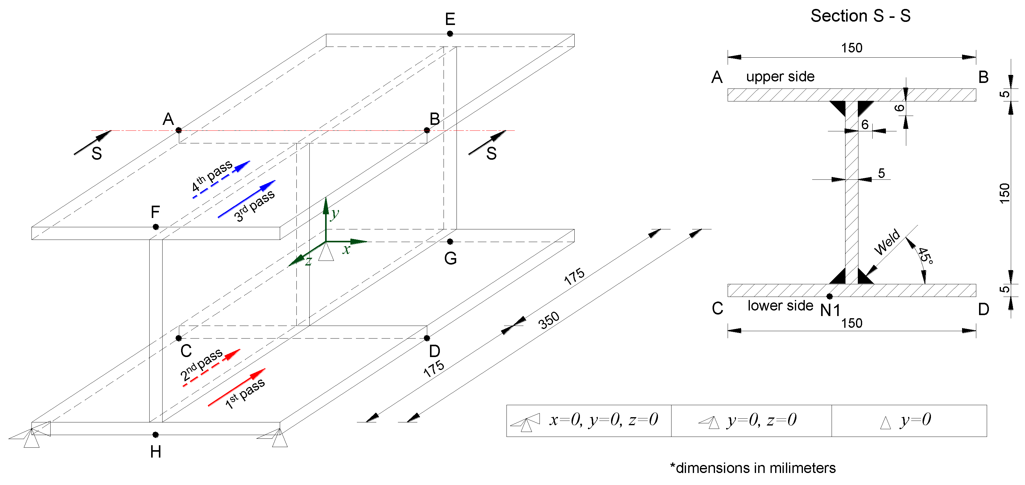
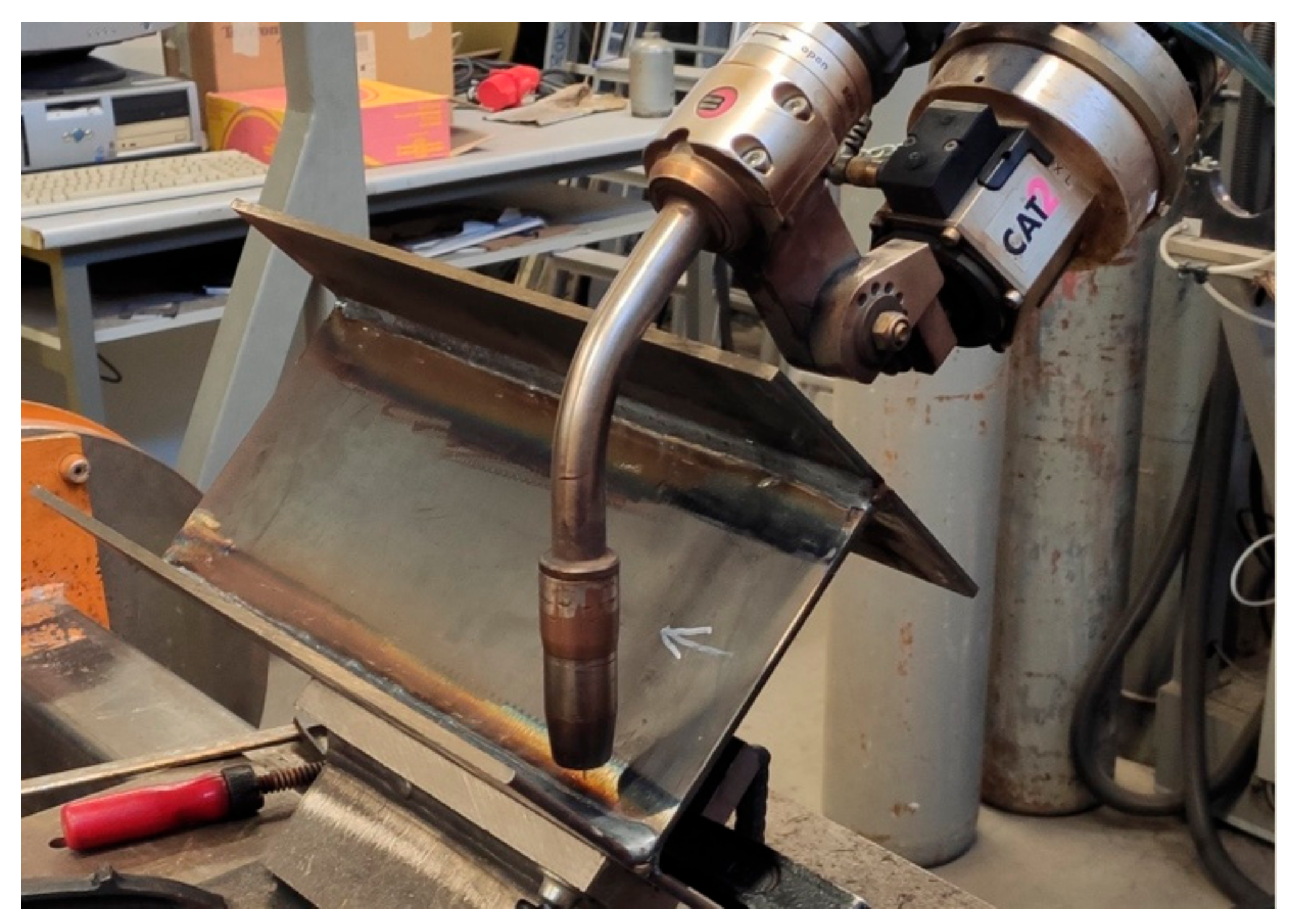
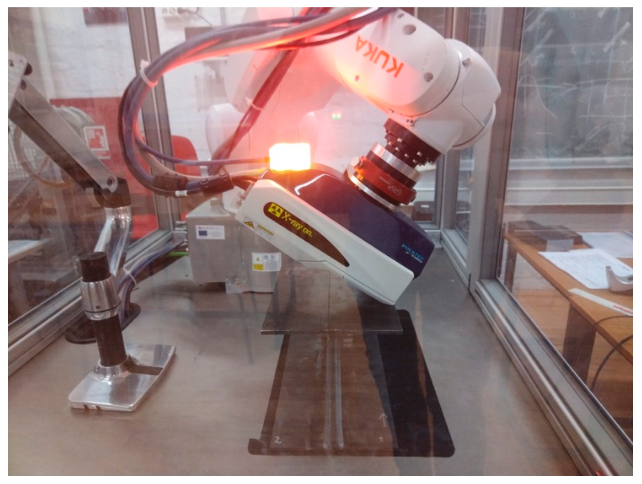
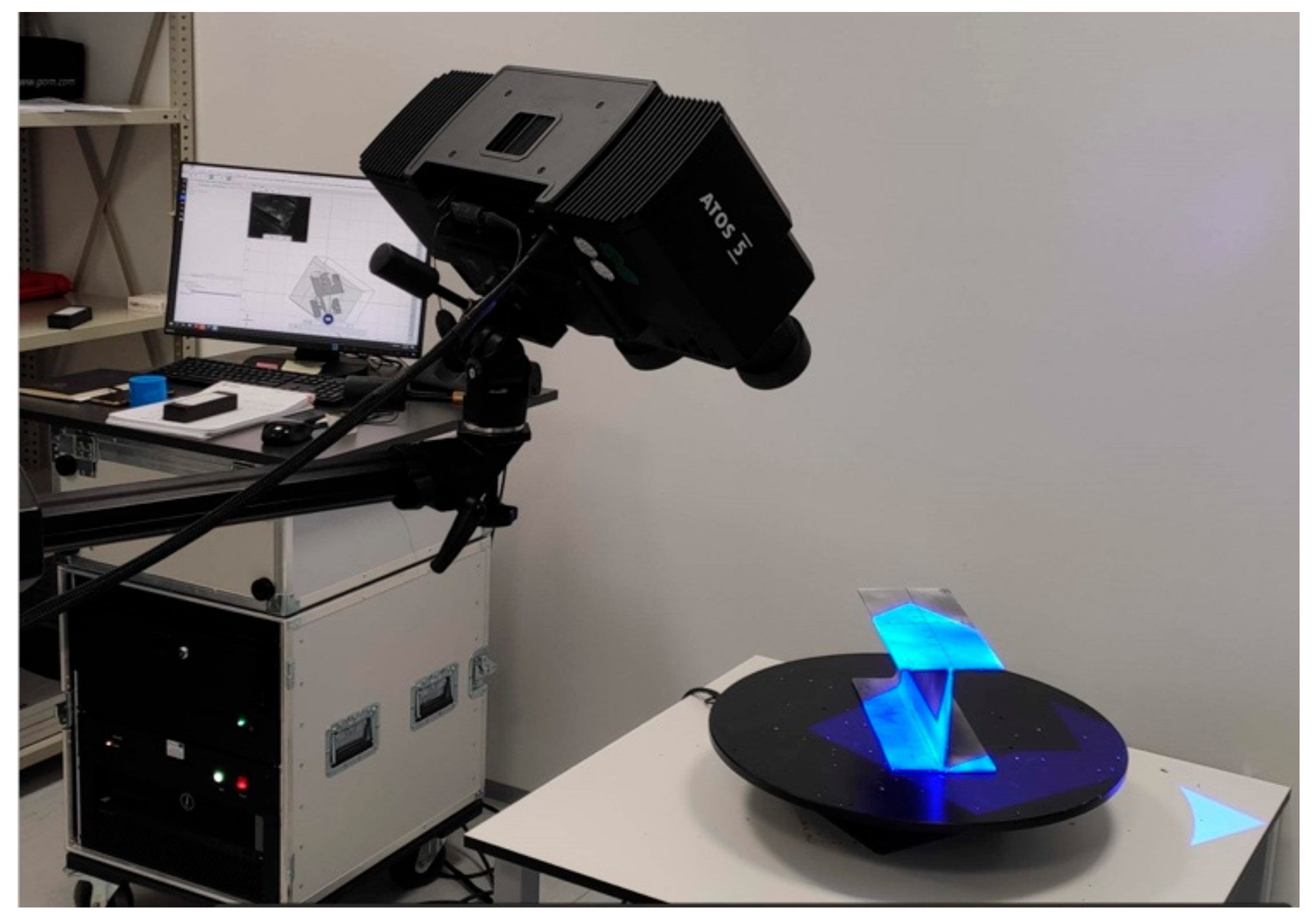
3. Experimental Investigations

Using the OTC Daihen Almega AX-V6 robotic welding station with the Daihen Varstroj WB-P500L power source, three steel plates of equal dimensions were welded to form an I-profile structure. The plates were produced from low-carbon steel 10025-2: S355J2+N, whose thermal and mechanical properties dependent on temperature and chemical composition were given in an earlier study [27]. The dimensions of the plates were 350 mm × 150 mm × 5 mm³. The plates were welded free, without mechanical stiffeners. The complete plates’ geometry and welding set-up are shown in Figure 1 and Figure 2. The MCAW welding procedure was completed without a gap between the plates. A working technique with a neutral welding gun inclination and tack welds at the beginning and end of each welding pass were used. The entire process of three-plate welding was performed in four single passes. All four passes were in the same direction with an intermediate cooling time of 180 s. The welding parameters were selected as follows: current 330 A, voltage 35 V and welding speed 10 mm/s. For welding, a wire with a diameter of 1.2 mm classified as EN ISO 17632-A: T 46 2 M M4, a shielding gas composition in accordance with ISO 14175: M24 (93%Ar/6%CO₂/1%O₂) and a gas flow of 20 L/min were chosen. The chosen type of welding wire ensures that the hydrogen content inside the weld does not exceed the amount of 5 mL H₂/100 g. To ensure uninterrupted metal transfer without spattering and without short circuits, a pulsed current was used.

After finishing the welding of the I-structure and cooling to ambient temperature, residual stresses were measured on the upper and lower sides of the model using the cosα X-ray diffraction method [28,29,30] (lines A–B, C–D, E–F and G–H, Figure 1). The X-ray measurement was performed with the device Pulstec μ-X360 (from Pulstec Industrial Co., Ltd., Hamamatsu, Japan) shown in Figure 3. The first measurement was carried out at a depth of 0.005 mm below the surface and showed quite large deviations and scattering of the results compared to the numerical simulation. The reason was probably the partial corrosion of the plate surfaces and the presence of residual stresses created during the manufacture of the plates. After that, residual stresses were measured at a depth of 0.015 mm, with the previous application of the electropolishing technique using the EP-3 device (from Pulstec Industrial Co., Ltd.), which achieved a good match between the experimental and numerical results.

The ATOS 5 12M XL (from GOM Metrology, Braunschweig, Germany) optical measurement system was used to measure I-profile deflections after welding, whose main characteristics are given below. Using advanced camera technology, a powerful light source and high-performance software, this system offers exceptional performance, especially when measuring challenging surfaces such as shiny and dark materials, intricate structures and edges. This technology significantly accelerates the measurement process while ensuring the accuracy of 3D data acquisition. The ATOS 3D optical scanner uses a triangulation method that employs a stereo camera integrated into the system sensor head and a projection unit. During the scanning process, the system uses fringe projection with a blue light equalizer to ensure the highest data quality. The sensor projects various fringe patterns onto the surface of the scanned object. This system uses multiple phase shifts based on the heterodyne principle to achieve exceptional sub-pixel accuracy. The collected points allow the tracking of the scanned object in the measurement space, correcting its orientation, and, finally, creating a 3D representation by joining the 2D images. During the process, the scanner must always have at least three reference points in its focus to ensure accuracy. In the case of our measurement, these reference points were restraint nodes (Figure 1). Since it is an industrial scanner, it is important to secure and stabilize the objects to be scanned. More about the applied method can be found in [31]. The measurement of deflections is shown in Figure 4.

4. Welding Numerical Simulation

The welding simulation was carried out using the finite element method and a sequential procedure [32], where two independent sequentially coupled thermal elastic–plastic analyses were performed: thermal and mechanical. In the thermal analysis, the weld length of all four passes of 1400 mm was divided into 140 sets of finite elements. Before starting the thermal simulation, all 140 sets of elements were deactivated. Using the element birth and death method [33], sets of elements were added one after the other imitating the motion of the electrode during welding. Each reactivated set of elements was first added in a very short period of time (10⁻⁷ s) and then subjected to heat flux for 1 s. After adding each individual set of elements and exposure to heat flux, the heat flux was turned off and the next set of elements was activated. After adding the 140th set of elements and exposing it to heat flux, the cooling process of the welded I-profile took place for 7500 s, which is enough to cool the workpiece to the ambient temperature, in this case 20 °C. It is important to note that uniformly distributed heat flux per each individual set of finite elements was used: Q = 5.13 × 10¹⁰ J/m³s. The usual Goldak heat flux [34], which is most commonly used in the numerical simulations of MAG welding, was omitted in this case. The reason is that the shape of the heat flux during MCAW significantly deviates geometrically [35] from the Goldak model. Since in the scientific literature, at least to the knowledge of these authors, there is no mathematical modification of Goldak’s heat flux suitable for MCAW simulation, a simplified heat flux with uniformly distributed heat throughout the weld volume was used, as stated above. A temperature-independent convection heat transfer coefficient h_c = 10 Wm⁻²K⁻¹ and a surface emissivity ε = 0.9 were assumed on the outer surfaces of the I-structure. The heat flux applied to each individual set of elements was calculated according to the expression:

$$Q=\frac{\eta UI}{V_H},$$

(1)

where η represents the efficiency of the MAG process, while U and I are welding voltage and current, respectively. The activated set of finite elements (weld volume) to which the heat was added is marked with V_H. In the thermal numerical simulation, the standardized value η = 0.8 was taken for the efficiency of the MAG process.

Having completed the thermal analysis, the space–time temperature distribution field obtained was used as a thermal load in the mechanical analysis, and in order to shorten the duration of the simulation, it was carried out simultaneously without using the element of birth and death technique. Although the complete I-profile was welded completely freely without mechanical stiffeners, in the mechanical simulation, stiffeners were added virtually in order to prevent the movement of the model as a rigid body. The plates and the weld material were modeled as a single body, without considering the effect of the gap between the plates [36]. Due to the lack of thermal and mechanical properties of the wire material, it was assumed that the material of plates and the filler material have the same thermophysical properties. Furthermore, the elastic-perfectly plastic behavior of the material was assumed in accordance with the von Mises criterion and the associated flow rule [37]. Since the welding wire melting process takes place rapidly and the exposure of the material to high-temperature cycles is very short, the creep of the material was not taken into account. Also, since the influence of phase transformations on the final state of residual stresses after welding in low-carbon steels is very small [38,39,40], phase transformations were not taken into account in this study. Taking into account the mentioned limitations in the numerical modeling of materials, the total strain tensor can be expressed in the form:

$$\left\{d{\epsilon }^{{}_{tot}}\right\}=\left\{d{\epsilon }^e\right\}+\left\{d{\epsilon }^p\right\}+\left\{d{\epsilon }^{th}\right\},$$

(2)

whereby in Equation (2) dε^e, dε^p and dε^th are elastic, plastic and thermal strain increments, respectively.

The entire I-profile model was created from 28,512 finite elements and the finite element mesh is shown in Figure 5. Due to the fact that the temperature gradients in the weld and its vicinity are very high, a very dense mesh of elements was used in that zone, which gradually decreased towards the edges of the plates. The mesh of the same density was used in both thermal and mechanical analyses. DC3D8 finite elements were used in the thermal analysis and they were converted to C3D8 ones in the mechanical analysis. All numerical simulations were performed using Abaqus software (version 6.14, ABAQUS Inc., Palo Alto, CA, USA).

5. Results and Discussion

In the framework of this research, special attention was paid to the creation of a finite element mesh and obtaining numerically accurate residual stress results. It is well known that mesh finite elements in the weld and its immediate surroundings must be very dense, while the rest of the model can be created with a sparser mesh due to smaller temperature gradients. A dense finite element mesh significantly increases the number of model elements, which requires considerable computer resources. In this paper, the convergence of the results of temperatures and residual stresses was limited to the very demanding area of the weld and its vicinity and was controlled by applying the submodeling technique through a global–local approach. It is important to point out that the number of finite elements of the submodel was 25,272, while on the other hand, the same volume in the area of the global model only contained 2656. Also, it can be confirmed that all the elements of the submodel were regular with equal aspect ratios, which was not the case with the global model. This avoids elongated elements that can give a worse solution. The area of the submodel includes the central part of the I-profile with the following dimensions: length (in z direction) 30 mm, width 58 mm (in x direction) and height 160 mm (in y direction). The coordinate system is shown in Figure 1 and the area of submodeling as well as the mesh details of the submodel in Figure 5.

Figure 6a shows a comparison of the temperature histories of the arbitrarily selected point N1 (Figure 1) for the global model and the submodel, and it is evident that there are no deviations in temperatures. Figure 6b shows the temperature profile of the submodel and global model on the lower side of the I-profile (lines C–D, Figure 1), whereas the deviations are less than 1%. Temperature histories and cooling curves refer to the time 215 s from the start of welding, i.e., after completion of the first weld pass and 180 s of cooling. Since the temperature difference between the submodel and the global model is very small, it can be concluded that the mesh of the global model was well-designed for the case of thermal analysis.

Figure 7a shows a comparison of the longitudinal residual stress (residual stress in the welding direction) of the submodel and the global model, and it is evident that the difference in the amount of stress is negligible. Figure 7b shows transversal residual stresses (stresses perpendicular to the welding direction) and it is evident that the difference in stresses is still acceptable. Both figures show the residual stress along lines C–D (Figure 1) on the lower side of the I-profile. Since the differences in the residual stresses of the global model and the submodel are within acceptable limits, it can be concluded that the mesh of the global model was dense enough and acceptable for the mechanical analysis.

Figure 8a–d shows comparisons of numerically calculated and X-ray experimentally measured values of residual stresses on the upper surface of the I-model. Figure 8a shows experimentally measured values of longitudinal residual stresses versus numerically obtained ones along lines A–B, Figure 1. It can be seen that the stresses in the welding zone are of a tensile character and less than the nominal yield stress value (355 MPa). Longitudinal stresses change to tensile ones towards the edges of the plates as shown in the numerical simulation and experimental measurement. Figure 8b shows the transversal stresses along lines A–B, Figure 1, and it is evident that in absolute terms, the transversal stresses are significantly smaller than the longitudinal ones. Also, from an insight into numerical and experimental measurements, it can be said that transverse residual stresses exist mainly in the weld zone, while they decrease towards the edges of the plates. Figure 8c shows numerically obtained longitudinal residual stress in comparison with X-ray diffraction measurements along lines E–F. Figure 8d shows the numerically obtained transverse residual stress in comparison with experimental measurements. It can be seen that the stresses are mostly equal and stable along the length of lines E–F, but drop sharply near the end of the plates.

Figure 9a–d show numerical and experimental amounts of residual stresses on the lower side of the I-model, analogous to Figure 8a–d. It can be seen that the corresponding stresses are very similar on both the upper and lower sides of the model. The reason is that the cooling time between welding passes is large enough and is equal between each welding pass. Also, the height of the middle plate of the I-profile is 150 mm, which is a sufficient distance between the welds for the plates to cool down sufficiently before the next welding pass. Figure 10a,b show full-field distributions of the longitudinal and transversal residual stresses after numerical simulation.

Figure 11 shows the deflections of the I-profile on the lower side of the model (Figure 1) along lines C–D on the lower side of the model. The measured deflections are about 12% higher compared to the numerically obtained values. The reason for the deviation can be attributed to the simplified heat-flux model used, which is very expressive when welding thin plates. The same reason leads to the deviation of numerical and experimental stresses.

6. Conclusions

Within this research for the case of MCAW welding for the I-profile structure, the residual stresses were numerically simulated and experimentally measured by the X-ray diffraction method. The conclusions are as follows:

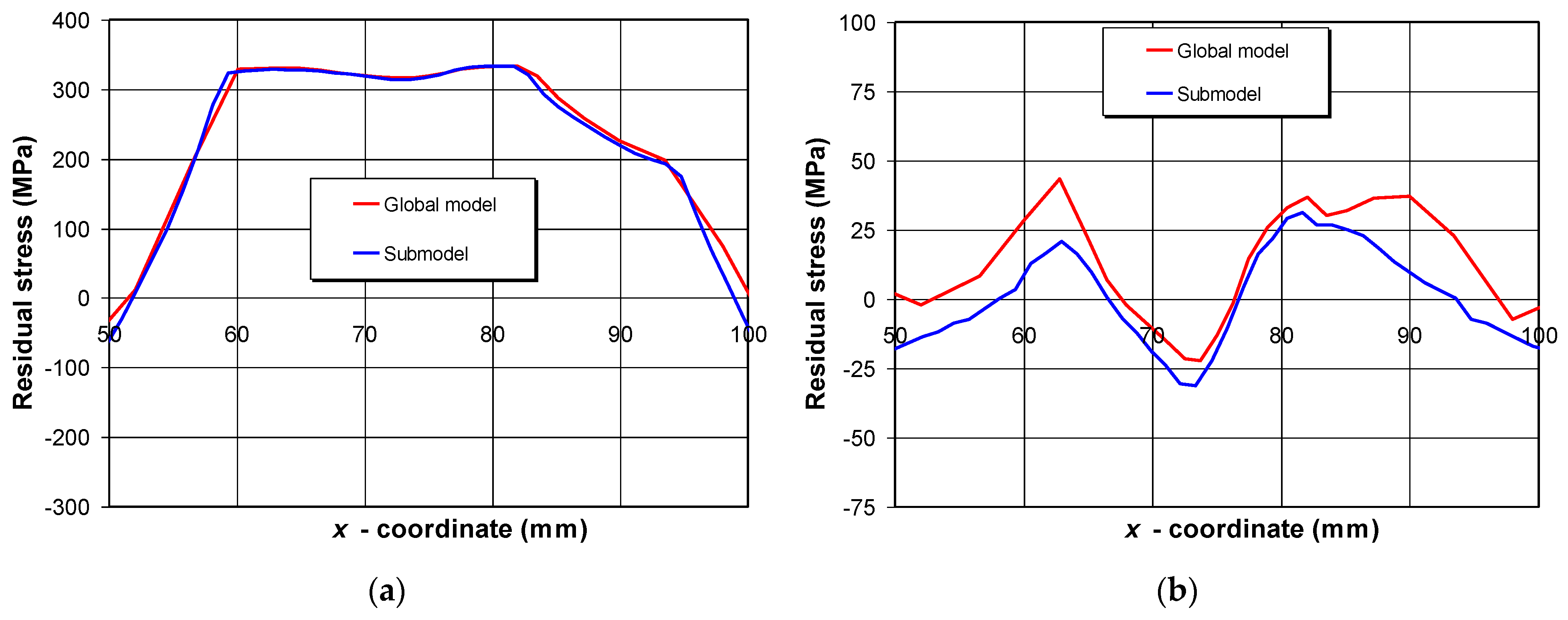
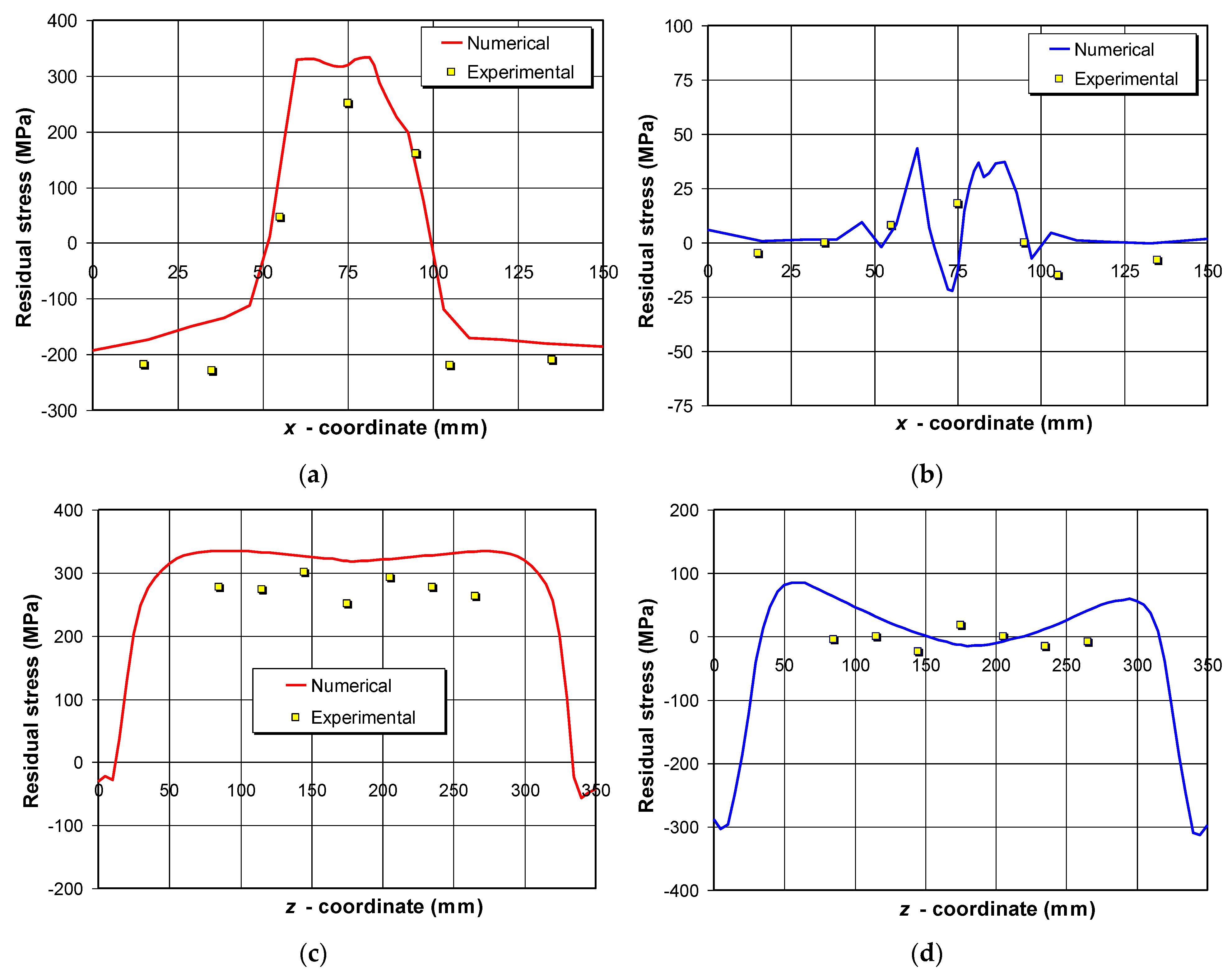
• Longitudinal residual stresses are dominant in the weld zone and the immediate vicinity and are tensile in nature. Moving away from the weld zone, tensile residual stresses change to compressive stresses toward the ends of the plates;
• Transversal residual stresses appear in the weld zone and its immediate vicinity, and completely disappear towards the ends of the plate;
• Residual stresses on the upper surface of the I-profile are almost identical to the stresses on the lower surface since the time between the weld passes is long enough for the material to cool down significantly;
• The experimental results obtained by the X-ray method are in good correlation with the numerical results;
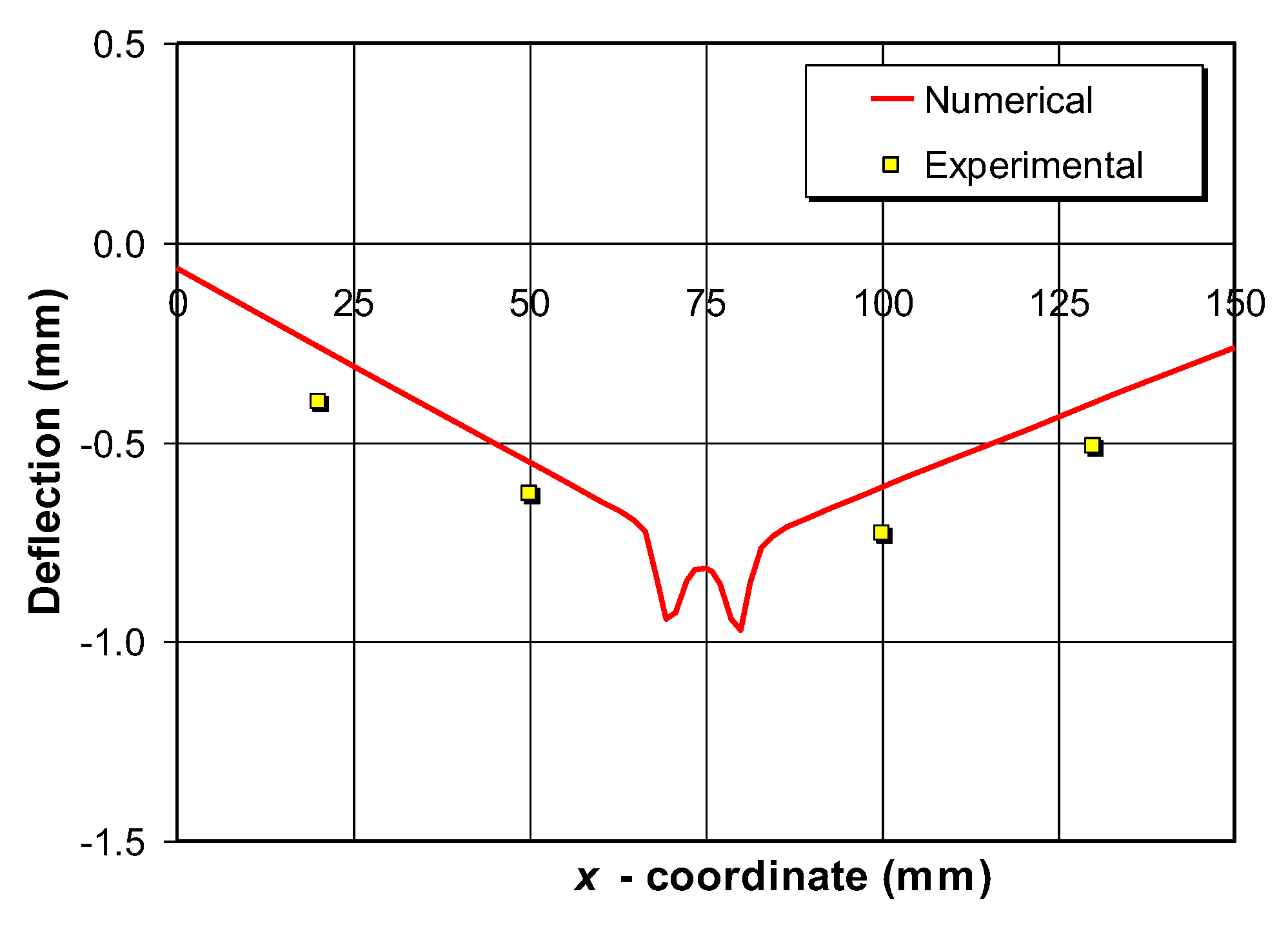
• The experimental results obtained by the 3D scan deflections follow the numerical results well.

References

1. Kik, T.; Moravec, J.; Švec, M. Experiments and Numerical Simulations of the Annealing Temperature Influence on the Residual Stresses Level in S700MC Steel Welded Elements. Materials 2020, 13, 5289. [Google Scholar] [CrossRef] [PubMed]
2. Lorza, R.L.; García, R.E.; Martinez, R.F.; Martinez Calvo, M.Á. Using Genetic Algorithms with Multi-Objective Optimization to Adjust Finite Element Models of Welded Joints. Metals 2018, 8, 230. [Google Scholar] [CrossRef]
3. Baruah, S.; Singh, I.V. A framework based on nonlinear FE simulations and artificial neural networks for estimating the thermal profile in arc welding. Finite Elem. Anal. Des. 2023, 226, 104024. [Google Scholar] [CrossRef]
4. Zhou, Z.; Cai, S.; Chi, Y.; Wei, L.; Zhang, Y. Numerical analysis and experimental investigation of residual stress and properties of T-joint by a novel in-situ laser shock forging and arc welding. J. Manuf. Process. 2023, 104, 164–176. [Google Scholar] [CrossRef]
5. Ghafouri, M.; Amraei, M.; Pokka, A.P.; Björk, T.; Larkiola, J.; Piili, H.; Zhao, X.L. Mechanical properties of butt-welded ultra-high strength steels at elevated temperatures. J. Constr. Steel Res. 2022, 198, 107499. [Google Scholar] [CrossRef]
6. Neuvonen, R.; Peltoniemi, T.; Skriko, T.; Ghafouri, M.; Amraei, M.; Ahola, A.; Björk, T. The effects of geometric and metallurgical constraints on ultra-high strength steel weldments. Structures 2023, 56, 104900. [Google Scholar] [CrossRef]
7. Sun, J.; Dilger, K. Reliability analysis of thermal cycles method on the prediction of residual stresses in arc-welded ultra-high strenghth steels. Int. J. Therm. Sci. 2023, 185, 108085. [Google Scholar] [CrossRef]
8. Sepe, R.; Giannella, V.; Greco, A.; De Luca, A. FEM Simulation and Experimental Tests on the SMAW Welding of a Dissimilar T-Joint. Metals 2021, 11, 1016. [Google Scholar] [CrossRef]
9. Božić, Ž.; Schmauder, S.; Wolf, H. The effect of residual stresses on fatigue crack propagation in welded stiffened panels. Eng. Fail. Anal. 2018, 84, 346–357. [Google Scholar] [CrossRef]
10. Gadallah, R.; Murakawa, H.; Shibahara, M. Investigation of thickness and welding residual stress effects on fatigue crack growth. J. Constr. Steel Res. 2023, 201, 107760. [Google Scholar] [CrossRef]
11. Dong, P.; Song, S.; Zhang, J. Analysis of residual stress relief mechanisms in post-weld heat treatment. Int. J. Press. Vessel. Pip. 2014, 122, 6–14. [Google Scholar] [CrossRef]
12. Cozzolino, L.D.; Coules, E.; Colegrove, A.P.; Wen, S. Investigation of post-weld rolling methods to reduce residual stress and distortion. J. Mater. Process. Technol. 2017, 247, 243–256. [Google Scholar] [CrossRef]
13. Deng, D.; Zhou, Y.; Bi, T.; Liu, X. Experimental and Numerical Investigations of Welding Distortion Induced by CO2 Gas Arc Welding in Thin-Plate Bead-on Joints. Mater. Des. 2013, 52, 720–729. [Google Scholar] [CrossRef]
14. Gannon, L.; Liu, Y.; Pegg, N.; Smith, M. Effect of welding sequence on residual stress and distortion in flat-bar stiffened plates. Mar. Struct. 2010, 23, 375–404. [Google Scholar] [CrossRef]
15. Wang, C.; Kim, Y.R.; Kim, Y.W. Comparison of FE models to predict the welding distortion in T-joint gas metal arc welding process. Int. J. Adv. Manuf. Technol. 2014, 18, 1637–1931. [Google Scholar] [CrossRef]
16. Shen, J.; Chen, Z. Welding simulation of fillet-welded joint using shell elements with section integration. J. Mater. Process. Technol. 2014, 214, 2529–2536. [Google Scholar] [CrossRef]
17. Kung, C.L.; Hung, C.K.; Hsu, S.M.; Chen, C.Y. Residual Stress and Deformation Analysis in Butt Welding on 6 mm SUS304 Steel with Jig Constraints Using Gas Metal Arc Welding. Appl. Sci. 2017, 7, 982. [Google Scholar] [CrossRef]
18. Ghafouri, M.; Ahola, A.; Ahn, J.; Björk, T. Welding-induced stresses and distortion in high-strength steel T-joints: Numerical and experimental study. J. Constr. Steel Res. 2022, 189, 107088. [Google Scholar] [CrossRef]
19. Perić, M.; Nižetić, S.; Garašić, I.; Gubeljak, N.; Vuherer, T.; Tonković, Z. Numerical Calculation and Experimental Measurement of Temperatures and Welding Residual Stresses in a Thick-Walled T-Joint Structure. J. Therm. Anal. Calorim. 2020, 141, 313–322. [Google Scholar] [CrossRef]
20. Raftar, H.R.; Ahola, A.; Lipiäinen, K.; Björk, T. Simulation and experiment on residual stress and deflection of cruciform welded joints. J. Constr. Steel Res. 2023, 208, 108023. [Google Scholar] [CrossRef]
21. Chen, B.Q.; Guedes Soares, C. Effects of plate configurations on the weld induced deformations and strength of fillet-welded plates. Mar. Struct. 2016, 50, 243–259. [Google Scholar] [CrossRef]
22. Li, G.; Feng, G.; Wang, C.; Hu, L.; Li, T.; Deng, D. Prediction of Residual Stress Distribution in NM450TP Wear-Resistant Steel Welded Joints. Crystals 2022, 12, 1093. [Google Scholar] [CrossRef]
23. Arivazhagan, B.; Kamaraj, M. Metal-cored arc welding process for joining of modified 9Cr-1Mo (P91) steel. J. Manuf. Process. 2013, 15, 542–548. [Google Scholar] [CrossRef]
24. Perić, M.; Garašić, I.; Štefok, M.; Jurica, M.; Osman, K.; Čikić, A.; Busija, Z. Numerical and experimental analysis of residual stresses in a metal-cored arc welded I-profile. In Proceedings of the 2023 8th International Conference on Smart and Sustainable Technologies (SpliTech), Split/Bol, Croatia, 20–23 June 2023; pp. 1–4. [Google Scholar] [CrossRef]
25. Yadav, G.P.K.; Bandhu, D.; Krishna, B.V.; Gupta, N.; Jha, P.; Vora, J.J.; Mishra, S.; Saxena, K.K.; Salem, K.H.; Abdullaev, S.S. Exploring the potential of metal-cored filler wire in gas metal arc welding for ASME SA387-Gr.11-Cl.2 steel joints. J. Adhes. Sci. Technol. 2023; in press. [Google Scholar] [CrossRef]
26. Bui, V.B.; Trinh, N.Q.; Tashiro, S.; Suga, T.; Kakizaki, T.; Yamazaki, K.; Lersvanichkool, A.; Murphy, A.; Tanaka, M. Individual Effects of Alkali Element and Wire Structure on Metal Transfer Process in Argon Metal-Cored Arc Welding. Materials 2023, 16, 3053. [Google Scholar] [CrossRef]
27. Perić, M.; Garašić, I.; Gubeljak, N.; Tonković, Z.; Nižetić, S.; Osman, K. Numerical Simulation and Experimental Measurement of Residual Stresses in a Thick-Walled Buried-Arc Welded Pipe Structure. Metals 2022, 12, 1102. [Google Scholar] [CrossRef]
28. Lin, J.; Ma, N.; Lei, Y.; Murakawa, H. Measurement of residual stress in arc welded lap joints by cosα X-ray diffraction method. J. Mater. Process. Technol. 2017, 243, 387–394. [Google Scholar] [CrossRef]
29. Hensel, J.; Nitschke-Pagel, T.; Dilger, K. On the effects of austenite phase transformation on welding residual stresses in non-load carrying longitudinal welds. Weld. World 2015, 59, 179–190. [Google Scholar] [CrossRef]
30. Sun, J.; Hensel, J.; Köhler, M.; Dilger, K. Residual stress in wire and arc additively manufactured aluminum components. J. Manuf. Process. 2021, 65, 97–111. [Google Scholar] [CrossRef]
31. Mašović, R.; Čular, I.; Vučković, K.; Žeželj, D.; Breški, T. Gear Geometry Inspection Based on 3D Optical Scanning: Worm Wheel Case Study. In Proceedings of the 2021 12th International Conference on Mechanical and Aerospace Engineering (ICMAE), Athens, Greece, 16–19 July 2021. [Google Scholar] [CrossRef]
32. Kong, W.; Huang, W.; Liu, X.; Wei, Y. Experimental and numerical study on welding temperature field by double-sided submerged arc welding for orthotropic steel deck. Structures 2023, 56, 104943. [Google Scholar] [CrossRef]
33. Meena, P.; Anant, R. On the Interaction to Thermal Cycle Curve and Numerous Theories of Failure Criteria for Weld-Induced Residual Stresses in AISI304 Steel using Element Birth and Death Technique. J. Mater. Eng. Perform. 2023; in press. [Google Scholar] [CrossRef]
34. Goldak, J.; Chakravarti, A.; Bibby, M. A new finite element model for welding heat sources. Metall. Trans. B 1984, 15, 299–305. [Google Scholar] [CrossRef]
35. Garašić, I.; Perić, M.; Tonković, Z.; Jurica, M.; Štefok, M.; Kik, T. Analysis of geometrical parameters for modification of Goldak heat source model in MCAW using Ar-CO2-O2 mixtures. In Proceedings of the 2023 8th International Conference on Smart and Sustainable Technologies (SpliTech), Split/Bol, Croatia, 20–23 June 2023; pp. 1–4. [Google Scholar] [CrossRef]
36. Bhatti, A.; Barsoum, Z.; Murakawa, H.; Barsoum, I. Influence of thermo-mechanical material properties of different steel grades on welding residual stresses and angular distortion. Mater. Des. 2015, 65, 878–889. [Google Scholar] [CrossRef]
37. Trupiano, S.; Belardi, V.G.; Fanelli, P.; Gaetani, L.; Vivio, F. A novel modeling approach for multi-passes butt-welded plates. J. Therm. Stress. 2021, 44, 829–849. [Google Scholar] [CrossRef]
38. Deng, D. FEM Prediction of Welding Residual Stress and Distortion in Carbon Steel Considering Phase Transformation Effects. Mater. Des. 2009, 30, 359–366. [Google Scholar] [CrossRef]
39. Wang, Y.; Feng, G.; Pu, X.; Deng, D. Influence of welding sequence on residual stress distribution and deformation in Q345 steel H-section butt-welded joint. J. Mater. Res. Technol. 2021, 13, 144–153. [Google Scholar] [CrossRef]
40. Feng, G.; Wang, H.; Wang, Z.; Deng, D. Numerical Simulation of Residual Stress and Deformation in Wire Arc Additive Manufacturing. Crystals 2022, 12, 803. [Google Scholar] [CrossRef]
Figure 1. Geometry of welded I-profile.
Metals 13 01766 g001
Figure 2. Welding set-up.
Metals 13 01766 g002
Figure 3. X-ray residual stress measurement.
Metals 13 01766 g003
Figure 4. Measurement of I-profile deflections.
Metals 13 01766 g004
Figure 5. Finite element mesh of I-profile.
Metals 13 01766 g005
Figure 6. Results of submodeling after thermal analysis: (a) temperature history of node N1 (Figure 1); (b) cooling profile along lines C–D, Figure 1.
Metals 13 01766 g006
Figure 7. Results of submodeling after mechanical analysis: (a) longitudinal residual stress along lines C–D, Figure 1; (b) transversal residual stress along lines C–D, Figure 1.
Metals 13 01766 g007
Figure 8. Residual stresses on the upper side of the I-profile, (Figure 1): (a) longitudinal residual stress along lines A–B; (b) transversal residual stress along lines A–B; (c) longitudinal residual stress along lines E–F; (d) transversal residual stress along lines E–F.
Metals 13 01766 g008
Figure 9. Residual stresses on the lower side of the I-profile, (Figure 1): (a) longitudinal residual stress along lines C–D; (b) transversal residual stress along lines C–D; (c) longitudinal residual stress along lines G–H; (d) transversal residual stress along lines G–H.
Metals 13 01766 g009
Figure 10. Full-field residual stress distributions: (a) longitudinal; (b) transversal.
Metals 13 01766 g010
Figure 11. I-profile deflection on lower side of I-profile along lines C–D.
Metals 13 01766 g011
Disclaimer/Publisher’s Note: The statements, opinions and data contained in all publications are solely those of the individual author(s) and contributor(s) and not of MDPI and/or the editor(s). MDPI and/or the editor(s) disclaim responsibility for any injury to people or property resulting from any ideas, methods, instructions or products referred to in the content.