Prediction of Hot Formability of AA7075 Aluminum Alloy Sheet

Abstract

A uniaxial high-temperature tensile test of an AA7075 aluminum alloy sheet was conducted using an established induction heating test system. Five different types of specimens were designed to obtain the stress–strain curves at different forming temperatures and strain rates so as to construct and modify the Johnson–Cook constitutive model. The uniaxial tensile test of different stress states was numerically simulated using ABAQUS finite element software, and the stress triaxiality and equivalent fracture strain parameters were extracted. The Johnson–Cook ductile fracture model was constructed, and an error evaluation scheme was designed to determine the best failure parameter combination. Based on the obtained Johnson–Cook ductile fracture model, finite element models of different strain paths were constructed, and theoretical forming limit curves at different temperatures and strain rates were obtained. The results of the Nakazima test and finite element simulation are mostly consistent, which confirms the reliability of the constructed fracture model and theoretical forming limit curves.

1. Introduction

In the automotive industry, the pursuit of safe and lightweight materials is unremitting [1,2,3]. The 7-series aluminum alloy has broad development prospects in the field of electric vehicles because of its light weight, high strength, good corrosion resistance, good formability, and excellent impact resistance. In addition, the aluminum alloy industry has a wide range of applications and unique advantages in aerospace, weaponry development, and mobile phone manufacturing. Therefore, the research progress of aluminum alloy-related processes has become a key factor related to the development of key industries [4,5,6,7,8,9]. Stamping is the main aspect of aluminum alloy sheet formation. Because the plasticity of 7-series high-strength aluminum sheets at room temperature is poor, warm-forming technology has been widely studied to effectively improve its formability.

A forming limit diagram is important for exploring the formability of materials [10,11]. At present, research on the forming limit test of materials at room temperature is quite mature. Using the system and standard for room-temperature tests, the high-temperature forming limit has also been thoroughly investigated. However, many external factors affect the test results under the conditions of high-temperature forming. In addition, the heating temperature, holding time, strain rate, friction, etc., are difficult to control precisely, which introduces higher requirements for the study of high-temperature forming limit [12,13]. Therefore, when studying the forming limit of materials under high-temperature conditions, many scholars have used theoretical calculations or FEM methods to construct forming limit prediction models. For the ductile fracture of an AA7075-T6 sheet, Yang et al. [14] proposed a new digital image correlation method to determine the ductile fracture parameters, and the forming limit diagram was constructed using a partition optimization method based on multiple sets of fracture parameters. Under the influence of different process parameters such as forming temperature, lubrication mode, and forming speed, Morchhale et al. [15] obtained the process curve by stretch forming. Stretch forming and deep drawing processes were conducted at 300 K and 673 K. The formability and strain limit of the IN625 alloy were determined, and a fracture-forming limit diagram (FFLD) was obtained. Goksen et al. [16] performed Nakazima tests on DKP-6112 and AZ31 Mg alloys using eight different types of specimens. The FLD results determined by the test were compared with numerical results and were found to be consistent. Through the wide-temperature-gradient tensile test and improved Erichsen test, Nasri et al. [17] studied the thermodynamic behavior and failure regularity of an A1050 aluminum alloy sheet in the forming process.

Generally, 7-series aluminum alloy is based on the heat treatment-forming-quenching (HFQ) process [18,19,20], and stamping is completed by means of a thermal simulation testing machine. In this study, to overcome unfavorable factors such as uncontrollable spatial distribution of the hot zone of the thermal simulation test machine and closed heating environment, AA7075 high-strength aluminum alloy was taken as the research object. The mechanical properties and fracture behavior characteristics of AA7075 aluminum alloy under different temperatures, strain rates, and stress states were obtained by induction heating. As a result, the Johnson–Cook fracture model was constructed. Based on the obtained Johnson–Cook ductile fracture criterion, finite element models of different strain paths were constructed, and theoretical forming limit curves at different temperatures and strain rates were obtained. The feasibility of the fracture model and theoretical forming limit curve was verified by a bulging test and simulation of an AA7075 aluminum alloy steel mold.

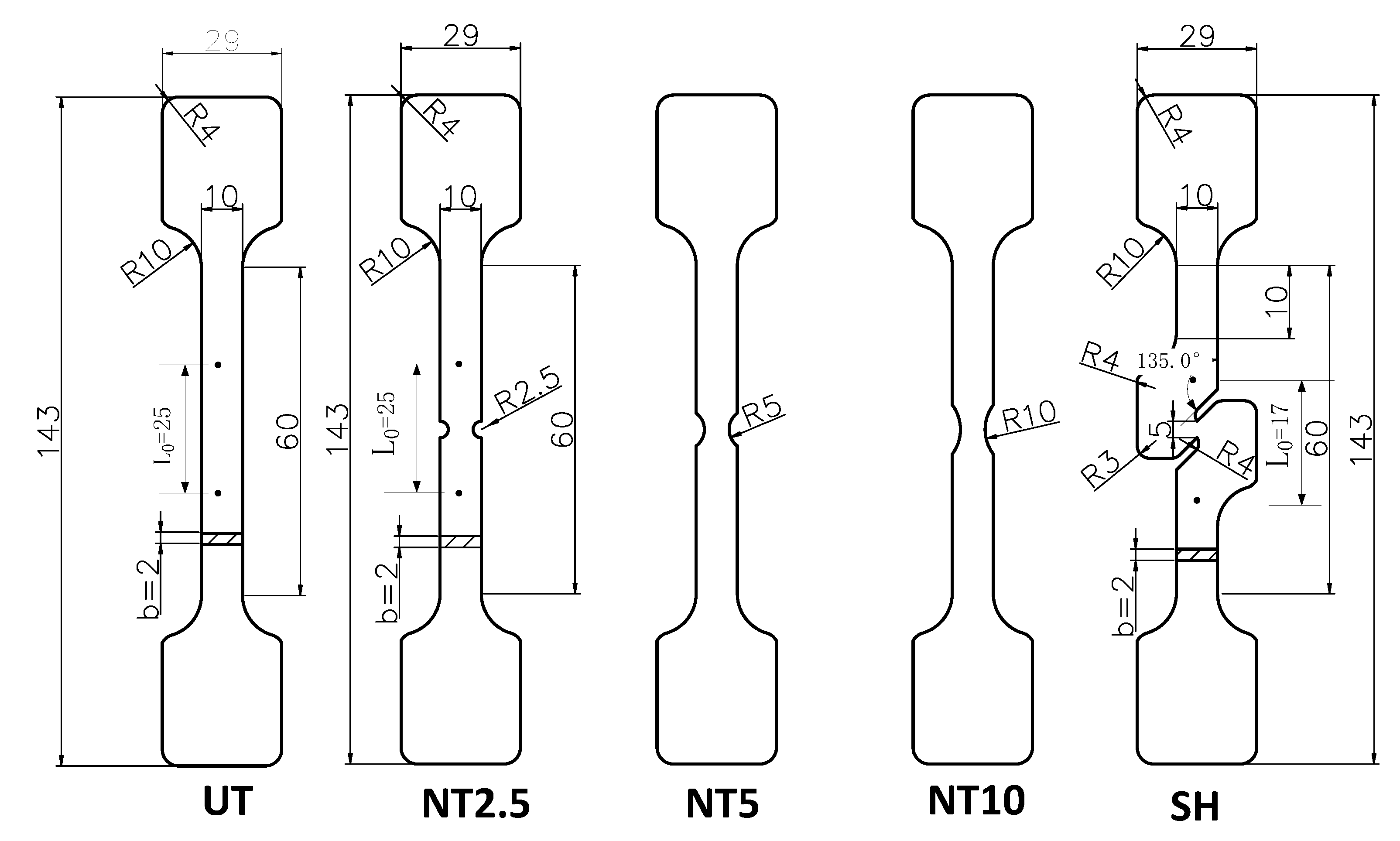
2. Uniaxial High-Temperature Tensile Test

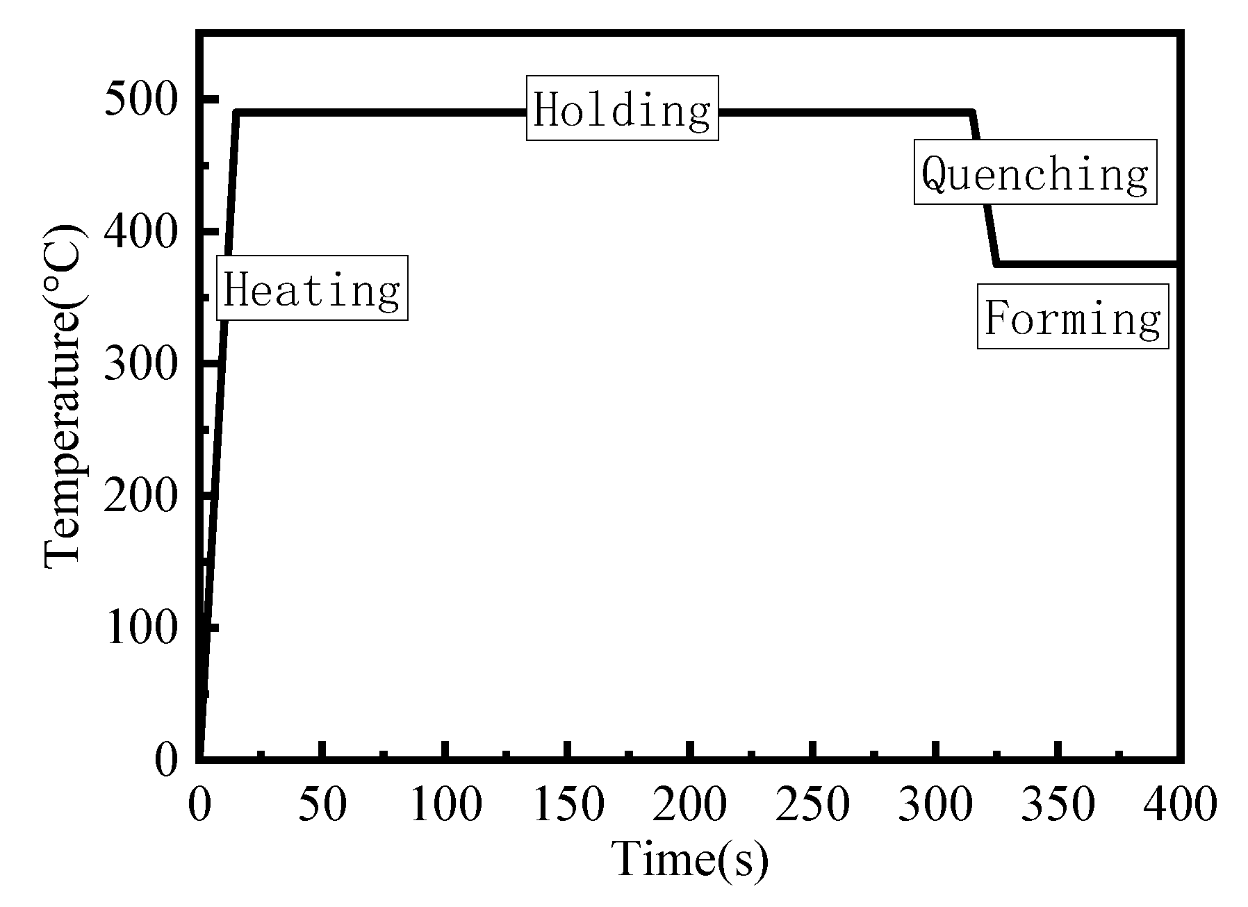
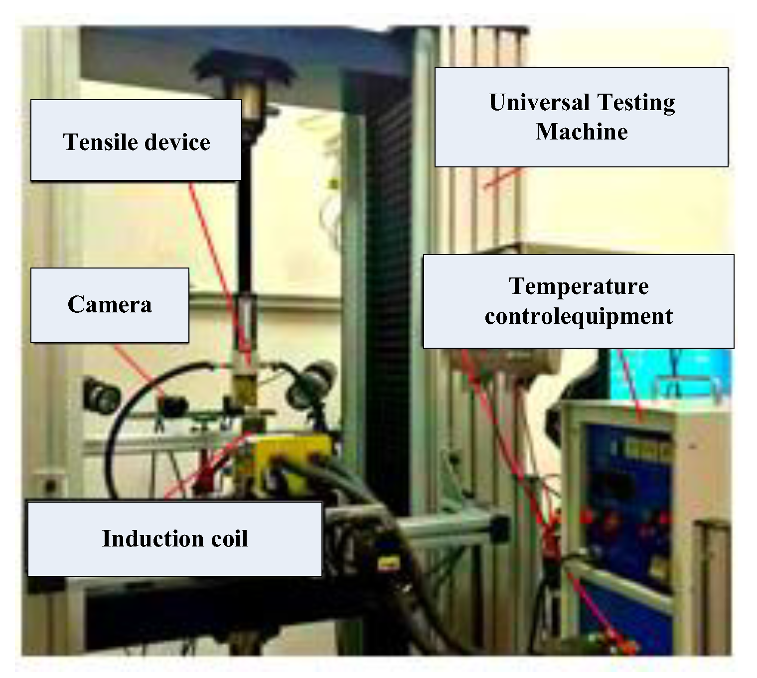
2.1. Test Scheme

The material used in the test was AA7075 cold-rolled high-strength aluminum alloy with a thickness of 2 mm. The chemical composition of the material is given in

Table 1. Chemical composition of AA7075 (wt.%).

Si	Fe	Cu	Mn	Mg	Cr	Zn	Ti	Al
0.17	0.22	1.57	0.11	2.46	0.20	5.63	0.09	-

. To obtain the basic material properties and fracture response under different stress states of AA7075 high-strength aluminum alloy, five different specimens were prepared, including a smooth specimen (UT), notched specimens (NT2.5, NT5, and NT10), and a shear specimen (SH). The shapes and specifications of the specimens are shown in Figure 1. The gauge section L₀ of the specimen needs to satisfy $5.65\sqrt{S_0}\ge 15$, and the length of the parallel section should not exceed $L_0+b/2$, where S₀ is the cross-sectional area of the specimen and b is its width. Depending on the size of b, the gauge length L₀ is 25 mm, and the parallel length is 60 mm [21].

Five different specimens were subjected to high-temperature uniaxial tensile tests based on the HFQ isothermal forming process. First, the specimens were heated to 490 °C (solid-solution temperature (SHT)) for a short time, and then maintained for 300 s. After the insulation treatment was completed, the temperature control threshold was adjusted to reduce the specimen temperature to the specified tensile test temperature. Finally, the specimens were subjected to isothermal tensile deformation until they fractured. Figure 2 shows the isothermal-forming HFQ hot forming process route map.

While simulating the process of transferring specimens from the heating furnace to the mold, the cooling time of each specimen was controlled within 10 s to prevent the long quenching time from affecting the mechanical properties of the specimens. However, the cooling water circuit set is in the fixture, and the thermal conductivity of the aluminum alloy is excellent. Thus, after testing, it was found that the heat-insulated specimen could be quickly cooled to the test temperature by quenching the mold at a cooling rate greater than 10 °C/s, without the need for an auxiliary cooling device.

Before the test, the prepared specimen gauge section was polished and smoothed, and black high-temperature matte paint was sprayed to obtain a black-and-white scatter diagram. Based on the black high-temperature matte paint coating, two symmetrical white spot patterns with a diameter of approximately 1 mm were plotted as the initial positions of the virtual extensometer, such as the black dot in Figure 1. A scatter diagram of the specimen was constructed to ensure that the scatter quality of the specimen was in the best state during the hot stretching process. The specimen was then fixed to a special fixture, and a 100 N preload was applied to reduce the systematic error caused by the specimen sliding during the test. Finally, the parameters of the hot tensile test system were adjusted, and the high-frequency power supply was turned on. A hot tensile test was conducted according to the HFQ hot forming process and related requirements. A field diagram of the hot tensile test system is shown in Figure 3.

The UT specimens were subjected to uniaxial tensile tests at temperatures of 375, 425, and 475 °C and strain rates of 0.01, 0.1, and 1/s. NT2.5, NT5, NT10, and SH specimens were tested at strain rates of 0.01, 0.1, and 1/s at 425 °C and at a strain rate of 0.1/s at 375, 425, and 475 °C. Each specimen was subjected to five test conditions. To ensure the accuracy of the test data, a minimum of two tests were conducted for each condition.

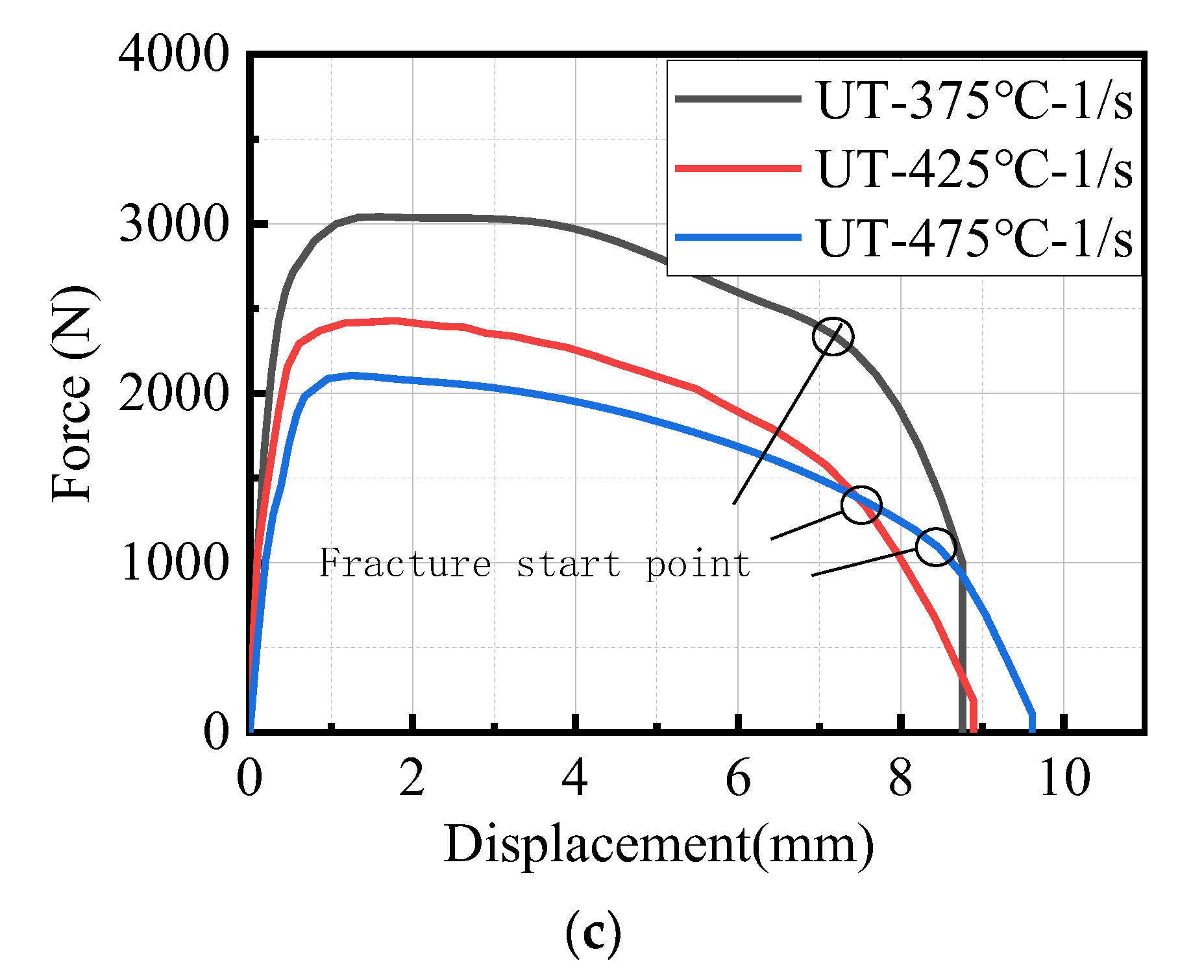
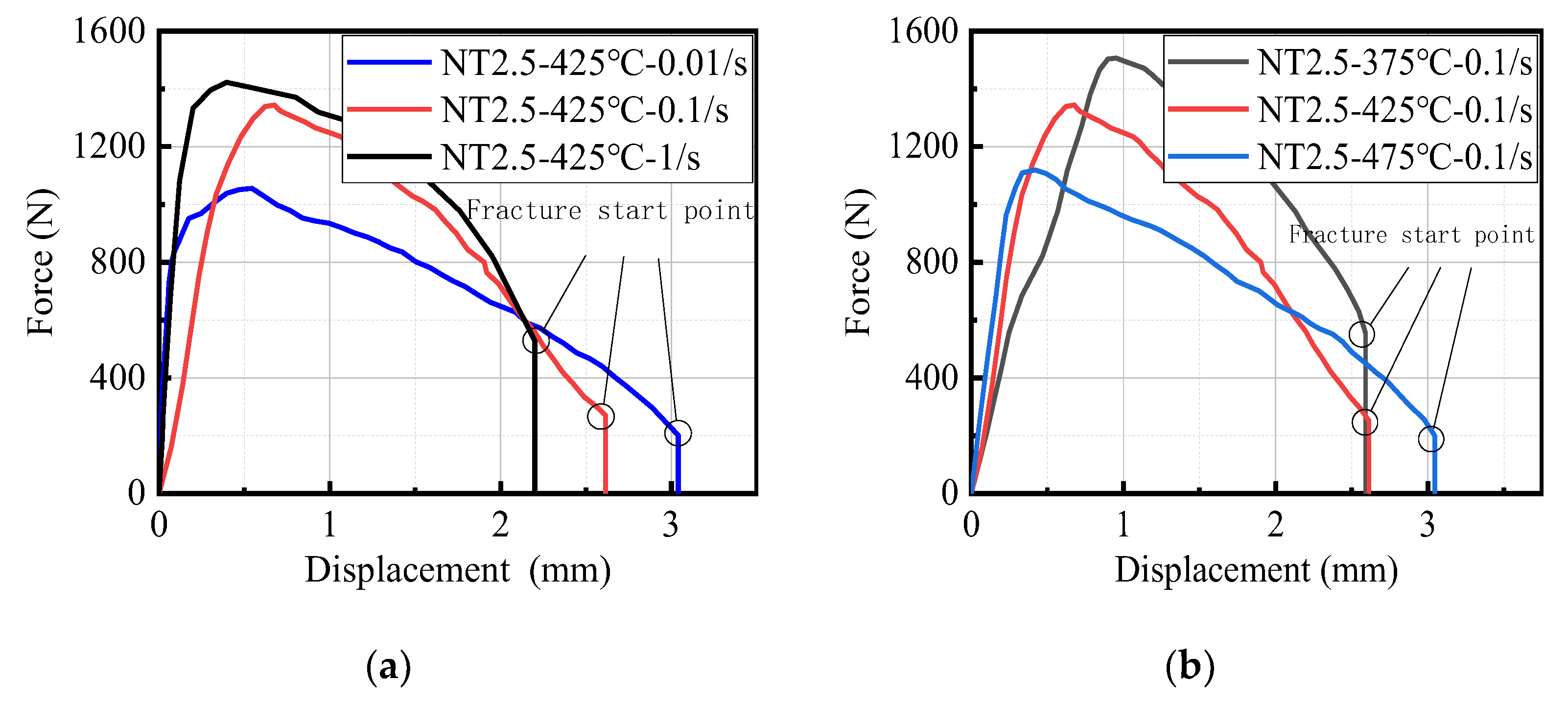
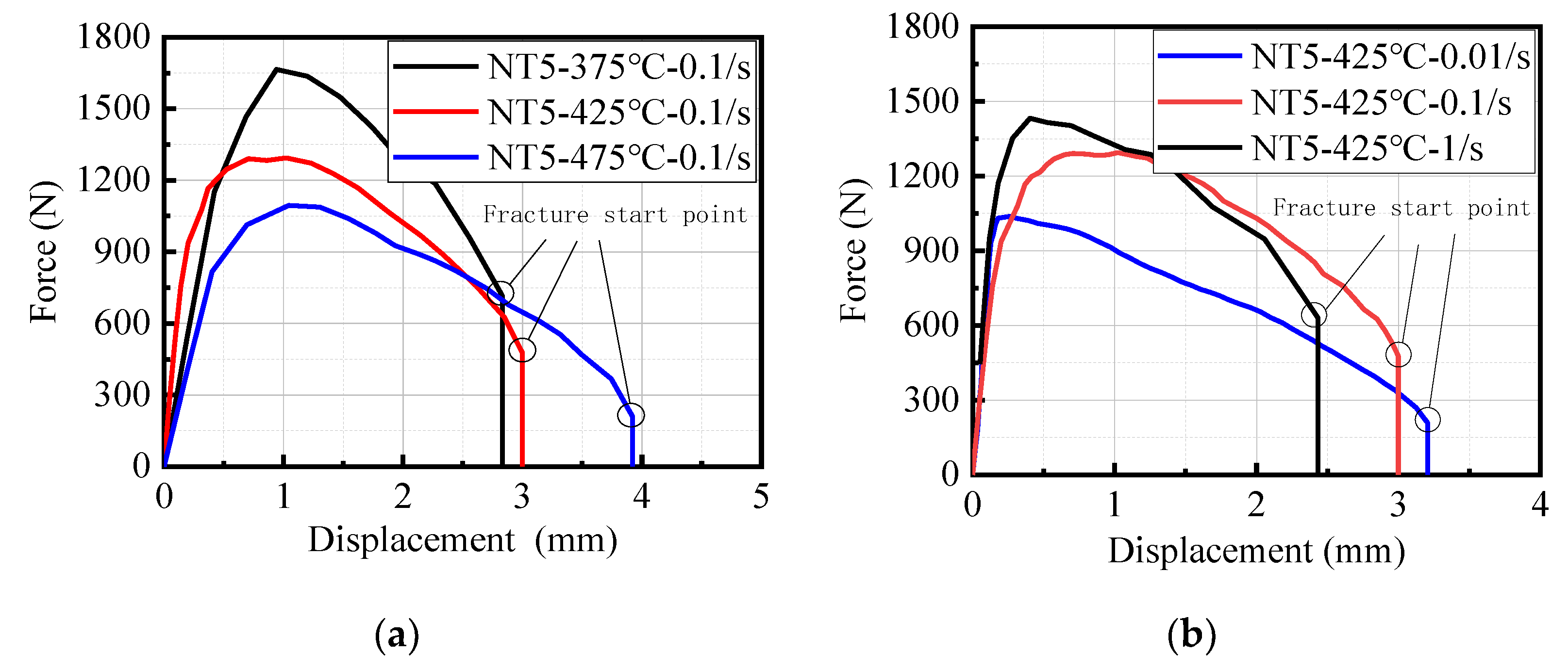
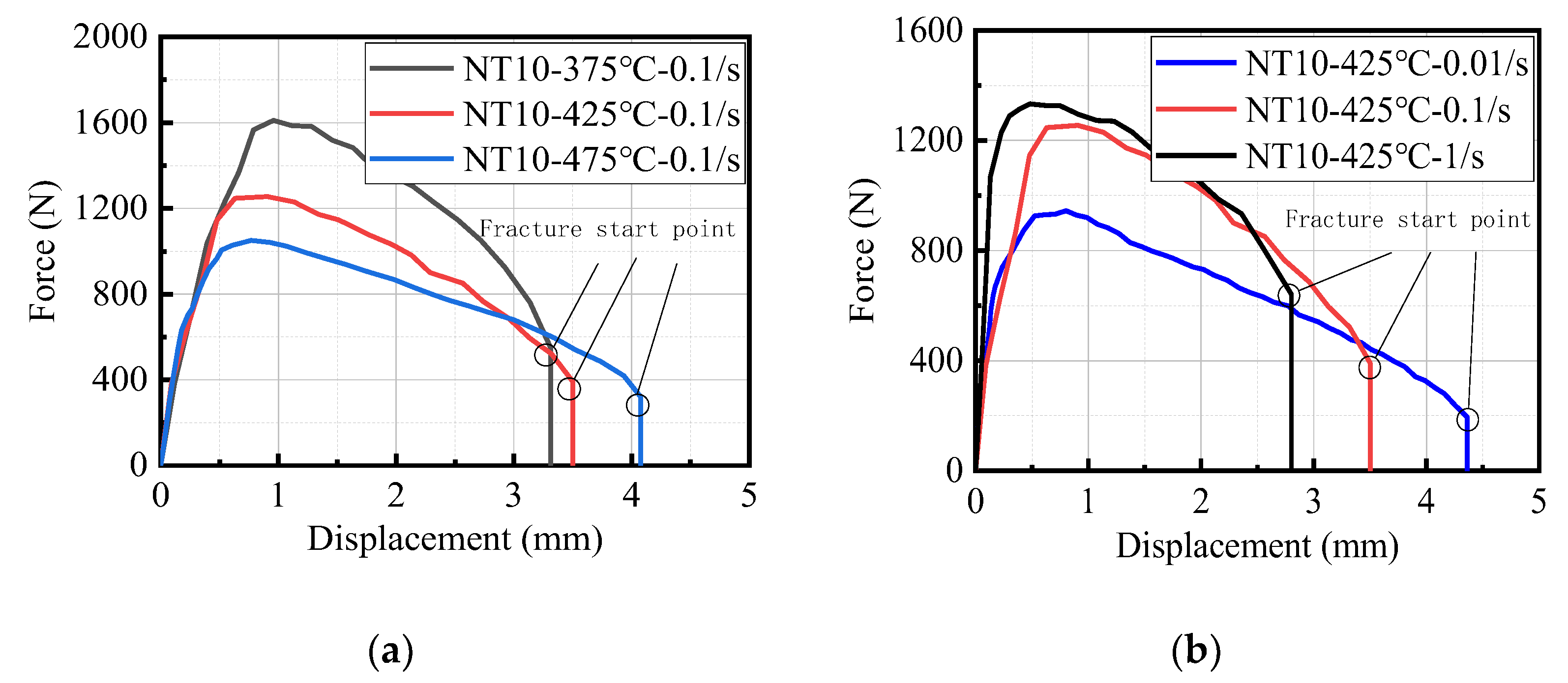
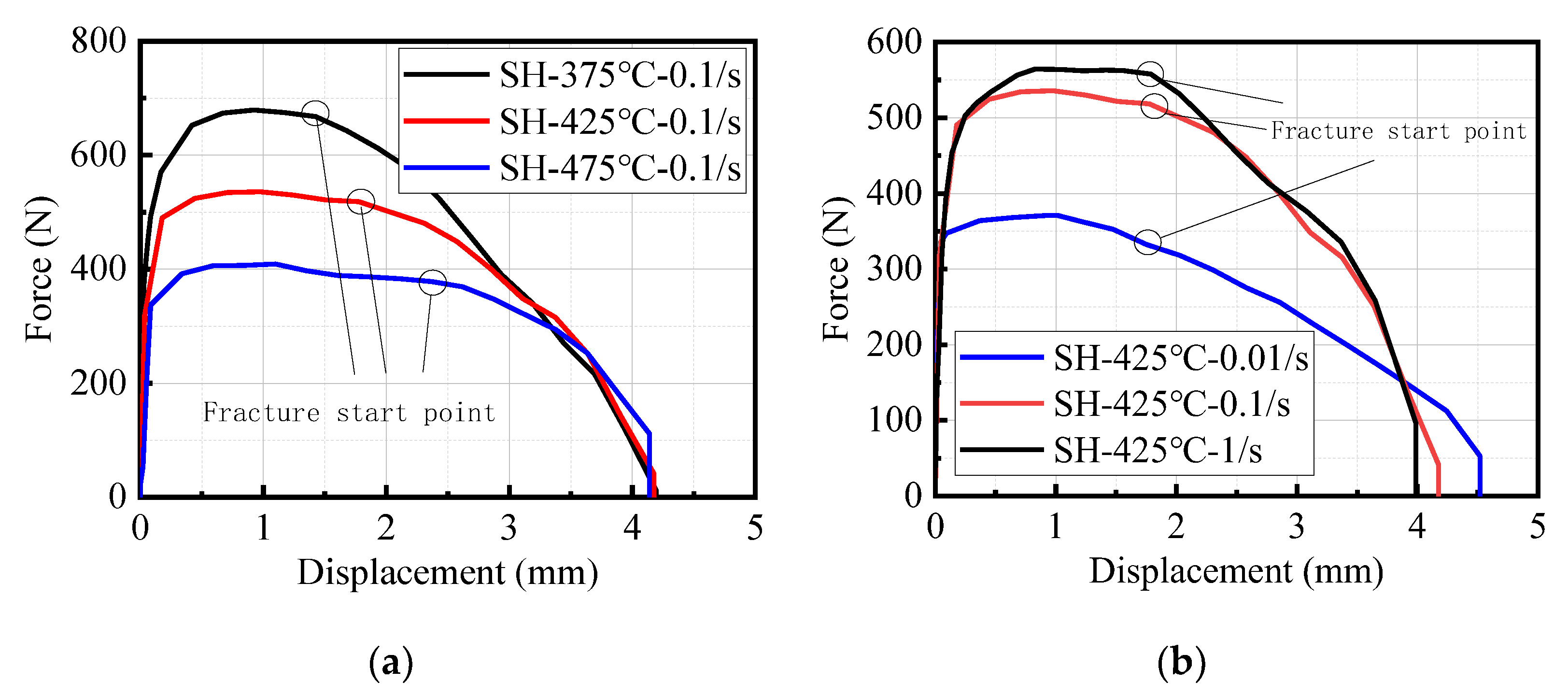
2.2. Force–Displacement Curves

The influence of changes in the strain rate and temperature on the ultimate load, fracture force, and fracture displacement of the material was explored. The test data were collated and fitted, and the force–displacement curves of five specimens of AA7075 aluminum alloy at a certain strain rate and temperature were obtained. The position of the fracture initiation point was marked according to the image taken by the DIC system. The results are presented in Figure 4, Figure 5, Figure 6, Figure 7 and Figure 8.

The ultimate load, fracture displacement, and fracture force were found to be related to the temperature and strain rate. Different specimens show the same characteristics: The higher the temperature, the lower the ultimate load and fracture force, and the greater the fracture displacement. The higher the strain rate, the higher the ultimate load and fracture force, and the smaller the fracture displacement.

3. Constitutive Model

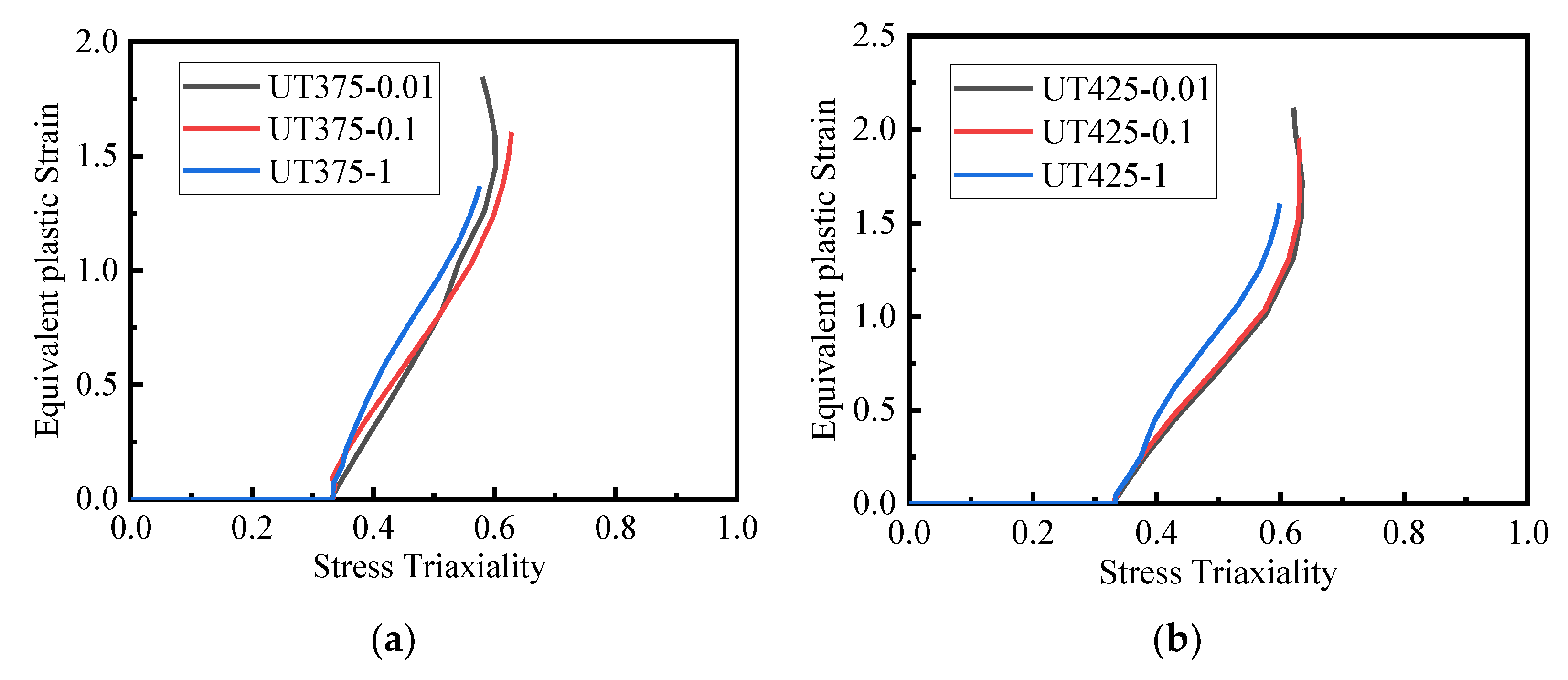
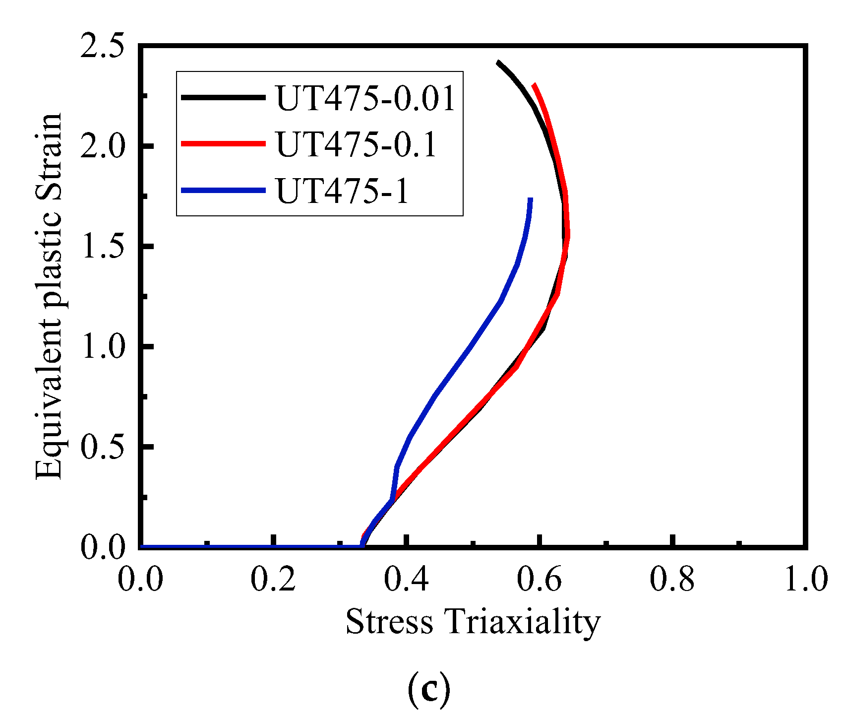
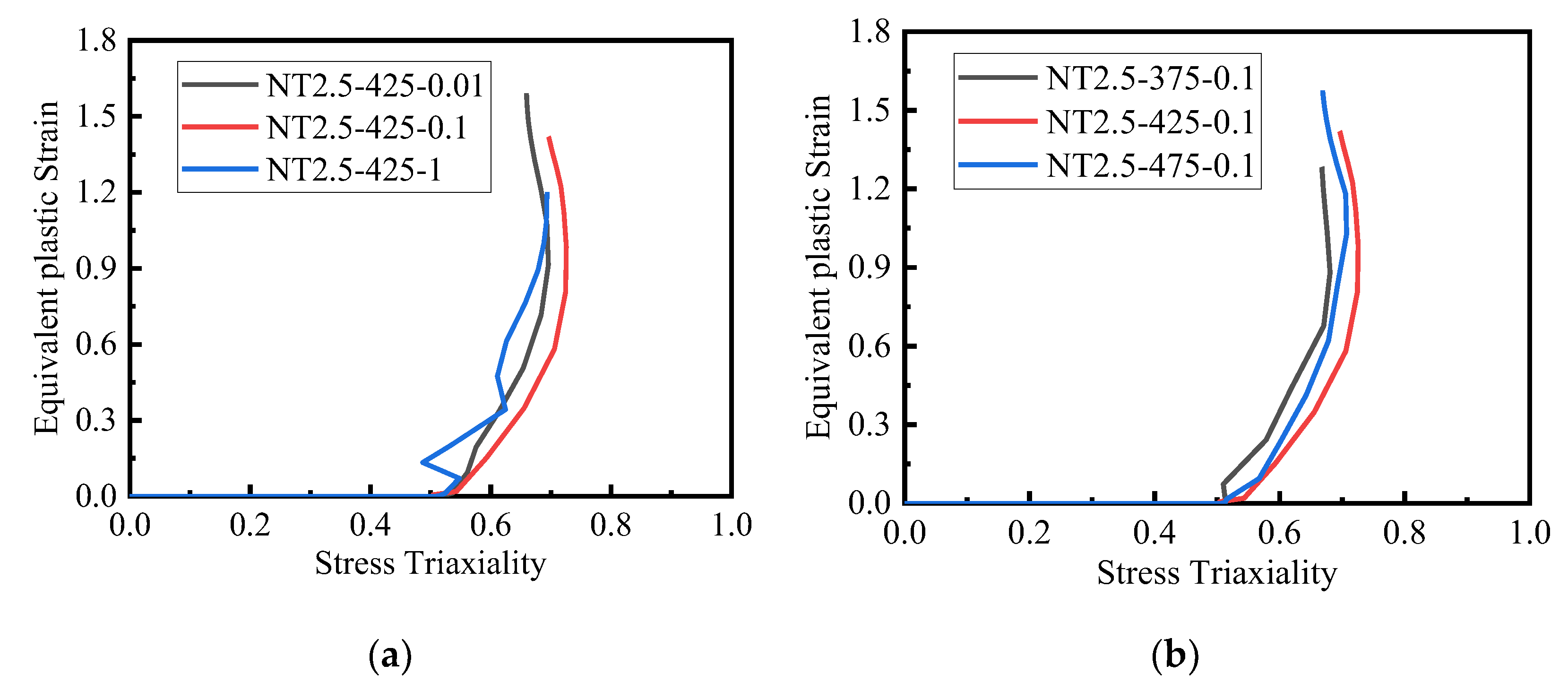
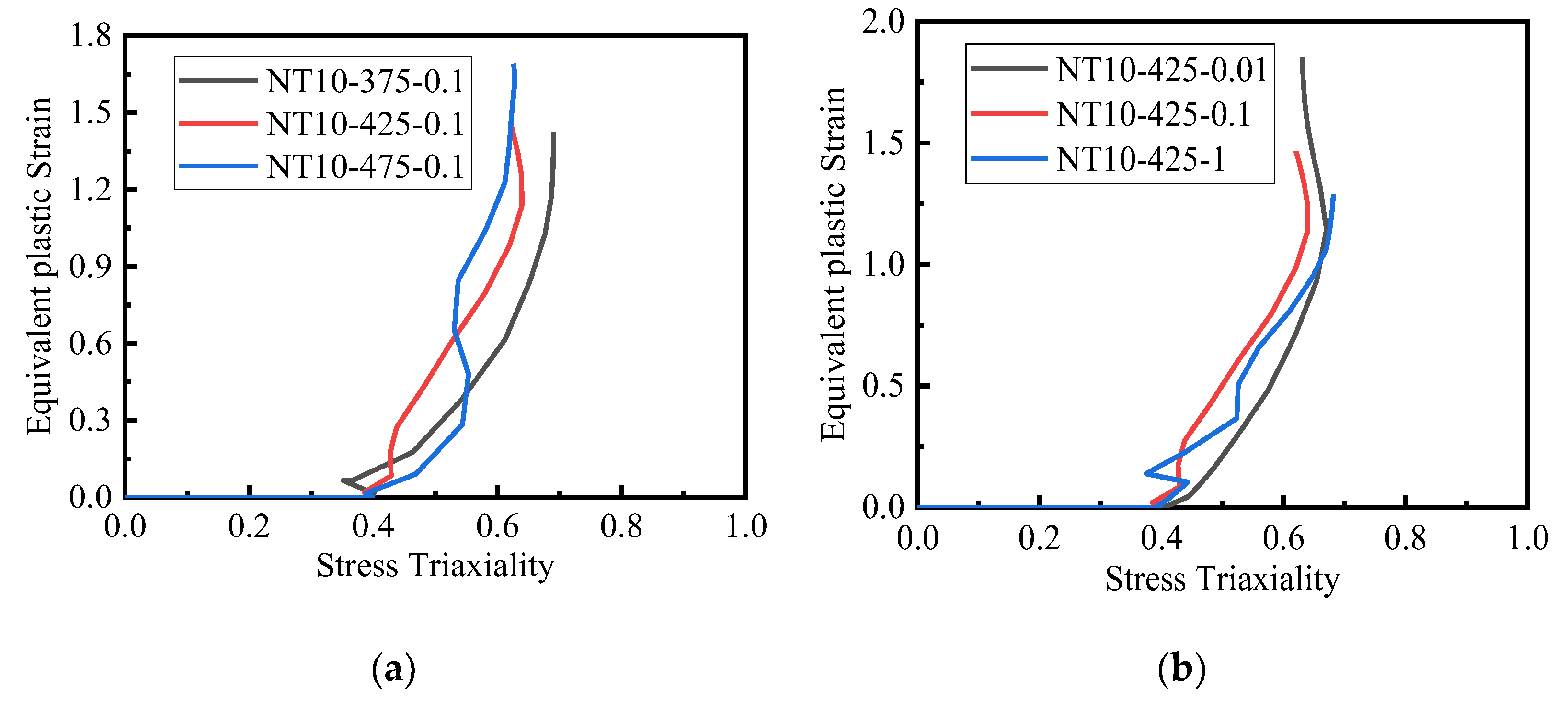
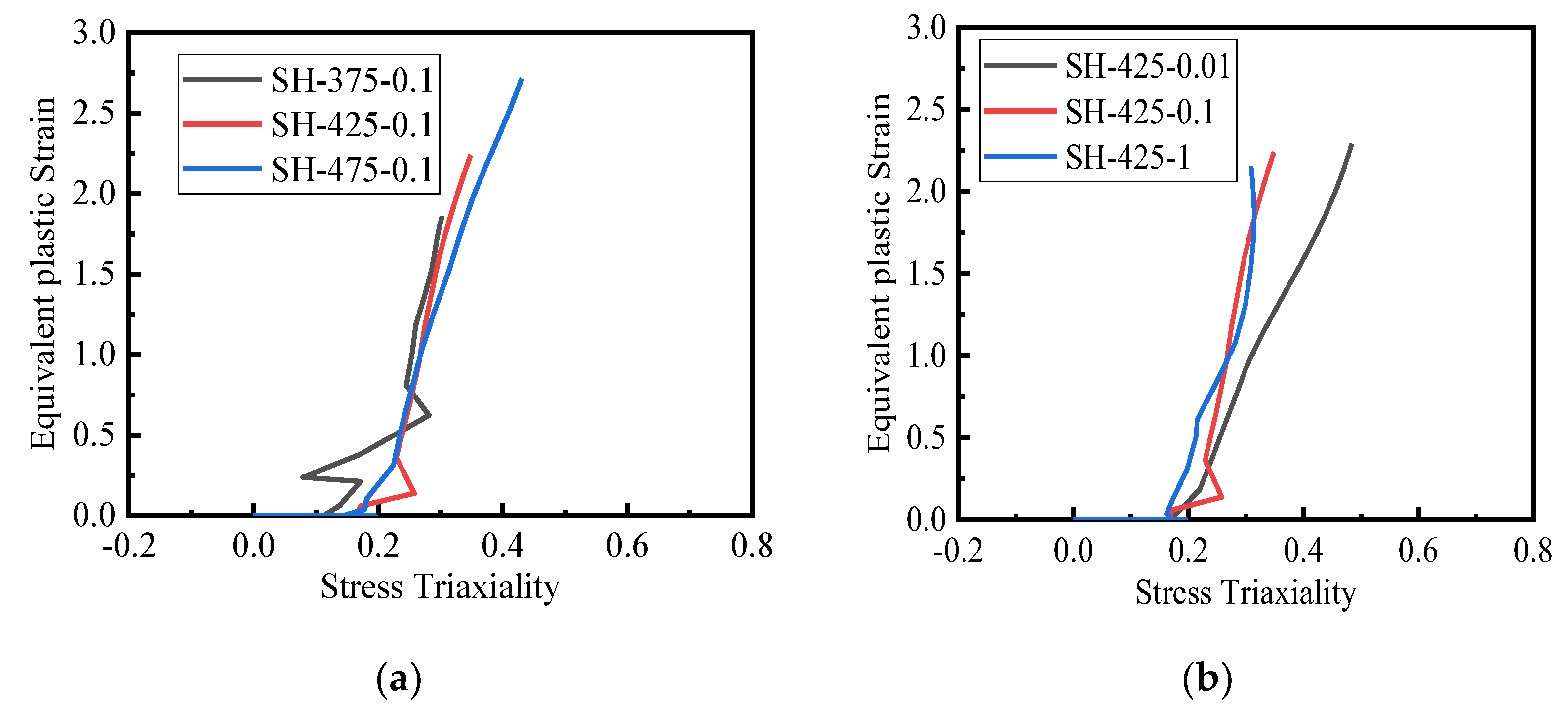
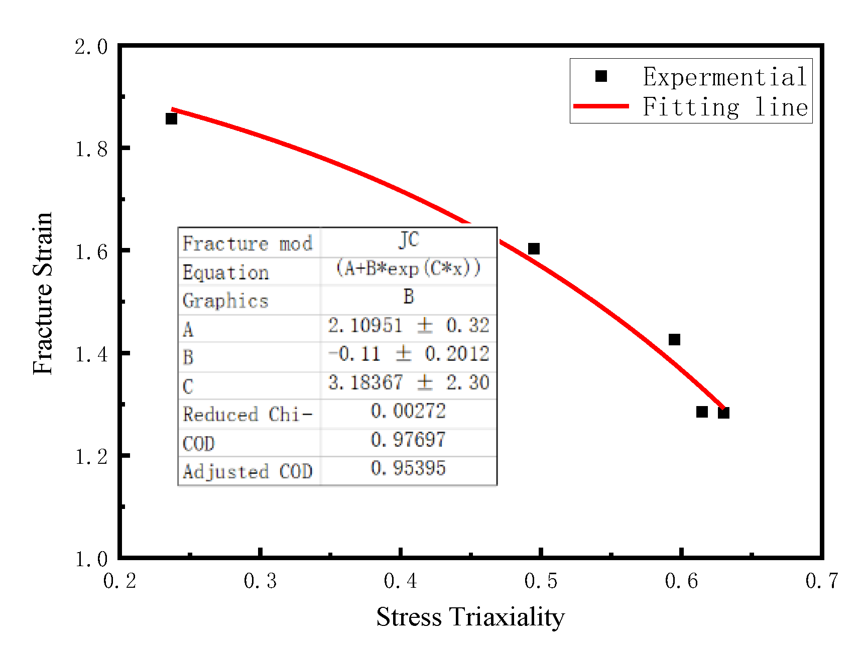
To accurately describe the mechanical properties of materials in different environments, a constitutive model is usually constructed using constitutive theory. The Johnson–Cook model is a phenomenological material flow rule proposed by Johnson and Cook in 1983 [22]. It couples plastic strain strengthening, strain rate sensitivity, and temperature softening. The expression is given by Equation (1).

$$\sigma =(A+B{\epsilon }^n)[1+C\ln \frac{\dot{\epsilon }}{{\dot{\epsilon }}_0}](1-{(\frac{T-T_r}{T_m-T_r})}^m)$$

(1)

where $\sigma$ is the equivalent stress of the material, $\epsilon$ is the equivalent plastic strain, $\dot{\epsilon }/{\dot{\epsilon }}_0$ represents the equivalent strain rate, $\dot{\epsilon }$ is the current strain rate, ${\dot{\epsilon }}_0$ is the reference strain rate, ${\dot{\epsilon }}_0$ = 0.001/s, Tr is the reference temperature, Tr = 25 °C, and Tm is the melting temperature, T_m = 550 °C. Finally, A, B, n, C, and m are five parameters to be calculated according to the stress–strain curve fitting at different temperatures and strain rates.

The original Johnson–Cook model considers that plastic strain hardening, strain rate sensitivity, and temperature softening are independent of each other. However, these three factors influence and restrict each other in the hot forming process of 7075 aluminum alloy. In fact, AA7075 aluminum alloy is less sensitive to low strain rates at room temperature. Further, according to the previous analysis, the strain rate significantly changes the mechanical properties of the material at high temperatures. Therefore, the strain rate sensitivity coefficient obtained by the conventional fitting method is less applicable at high temperatures. Therefore, the Johnson–Cook model should be corrected [23].

The necking stage of 7075 aluminum alloy is long, and the strengthening stage is short during high-temperature forming. The first item of the original Johnson–Cook model adopts the Holloman hardening model. This hardening model is a typical pure power-hardening model, and the fitting accuracy of a large necking deformation is poor. Therefore, the Holloman hardening model is modified to a more adaptable version of the Swift–Voce model. The Swift–Voce model is a hardening model that combines the Swift and Voce models using weighting coefficients. The form is expressed as Equation (2).

$$\sigma =[\alpha A{\epsilon }^n+(1-\alpha )(K+Q{e}^{-B\epsilon })]$$

(2)

The modified model is expressed as Equation (3).

$$\sigma =[\alpha A{\epsilon }^n+(1-\alpha )(K+Q{e}^{-B\epsilon })][1+C\ln \frac{\dot{\epsilon }}{{\dot{\epsilon }}_0}][1-{(\frac{T-T_r}{T_m-T_r})}^m]$$

(3)

where $\alpha$, A, n, K, Q, B, C, and m are undetermined parameters. The model was programmed into ORIGIN v.10.0 software. Each parameter was set to an initial value. Next, each curve was fitted, and the fitting results were collated and corrected. It is found that $\alpha$ changes synergistically with the strain rate. When $\dot{\epsilon }$ = 0.01/s, the $\alpha$ value is 0; when $\dot{\epsilon }$ = 0.1/s, the $\alpha$ value is 0.70337; and when $\dot{\epsilon }$ = 1/s, the $\alpha$ value is 0.73796. Here, A = 982.35250 MPa, n = 0.02377, Q = −2209.13513, and m = 1.03161. The three parameters of K, B, and C are related to the changes in temperature and strain rate, and the corresponding values are obtained by fitting, as shown in

Table 2. Fitted values of K, B, and C parameters.

Temperature (°C)	Strain Rate (/s)	K	B	C
375	0.01	92.07117	473.01661	3.00000
	0.1	−414.94421	115.57266	−0.12683
	1	328.87782	81.24024	−0.17783
425	0.01	259.48459	412.40667	0.50000
	0.1	−3.73651	107.83479	−0.16058
	1	−1058.39724	144.79391	0.16687
475	0.01	530.40297	338.87563	−0.14784
	0.1	309.89884	89.32858	−0.04666
	1	−691.78899	118.37685	0.28173

.

Figure 9 shows a comparison between the constitutive model fitting curve and the test curve at different strain rates. A good fit is observed from the figure.

4. Fracture Model

The Johnson–Cook fracture strain model is as follows.

$${\overline{\epsilon }}_f=[D_1+D_2\exp (D_3\eta )][1+D_4\ln (\frac{\dot{\epsilon }}{{\dot{\epsilon }}_0})][1+D_5(\frac{T-T_r}{T_m-T_r})]$$

(4)

The model consists of three parts: The first part shows the relationship between the equivalent fracture strain ${\overline{\epsilon }}_f$ and the stress triaxiality $\eta$. The second part shows the influence of the change in strain rate on the equivalent fracture strain ${\overline{\epsilon }}_f$. The third part shows the thermal softening effect on the ductility of the material. Here, D1, D2, D3, D4, and D5 are failure parameters.

In the Johnson–Cook fracture model, the reference strain rate ${\dot{\epsilon }}_0$ is set to 0.1/s, the reference temperature is set to 375 °C, the melting temperature T_m is 550 °C, and five failure parameters D1–D5 are calibrated using specimens with different stress states.

In the fracture model, the stress triaxiality is selected as the stress–state characterization parameter. The stress triaxiality can be directly calculated using the formula for a simple stress state, but a large necking phenomenon usually occurs during hot stretching until the fracture process. A material cannot be simply classified as a uniaxial tensile stress state near a fracture. At this time, the stress state is more complicated. The method adopted by many scholars is to extract the stress state parameters using finite element simulation [24,25,26]. In this study, ABAQUS/Standard finite element v.2022 software was used to model the gauge sections of different types of specimens. The C3D8R mesh type was used for mesh division, and the mesh of the main deformation parts of the notched specimen and the shear specimen was locally refined. The geometric model is illustrated in Figure 10.

After the simulation was completed, the experimental failure image and the FEM equivalent fracture cloud map of the fracture initiation time of different types of specimens at 375 °C and 0.1/s were extracted. The comparison results are shown in Figure 11.

To determine the behavior state of the material at the time of fracture initiation, the first two-dimensional image of the fracture was captured using the DIC system, and the macroscopic morphology of the specimen at the time of fracture initiation was observed. Compared with the equivalent plastic strain results of the FEM numerical simulation, it was found that the two were highly consistent. The types of specimens and the positions of the critical points were different. The surface center element nodes of the smooth plate specimens and the finite element models of the three notched specimens were determined and extracted as the critical points of fracture. In the shear specimens, the node of the equivalent plastic strain enrichment zone element below the notch was the critical point of fracture. The specific analysis is as follows: Considering the experimental failure image and simulation results at 425 °C and 0.1/s as an example, it can be seen from Figure 11a that necking occurs in the middle of the UT specimen. Further, the fracture gradually expands from the center to the outside. From Figure 11b–d, it is evident that the fracture surface of the three notched specimens is severely thinned and that the fracture surface cracks almost simultaneously. This result is consistent with the equivalent plastic strain distribution at the fracture surface in the simulation results. The position at which the shear specimen begins to break is shown in Figure 11e.

The stress triaxiality evolution process of the critical point at the fracture time of the five specimens was extracted. The results are presented in Figure 12, Figure 13, Figure 14, Figure 15 and Figure 16.

For the Johnson–Cook fracture model, only five failure parameters must be obtained for a full calibration. Based on the 44 sets of tests completed, the stress triaxiality and fracture strain values of five different shapes and specifications of the specimens at the reference temperature and strain rate were first extracted. The values of D1, D2, and D3 were then obtained by fitting. Subsequently, the data at the reference temperature and the non-reference strain rate were selected to calibrate the value of D4, which were the data corresponding to UT-375-0.01 and UT-375-1 specimens. Finally, data from one of the remaining 22 specimens were inserted into Equation (4) to obtain the data of D5, and a total of 44 groups of specimens were obtained.

For different specimen combinations, each set of data contains five different types of specimens, but only D4 and D5 need to be obtained. The specimen number is represented by U_i,j,k, where angle index i is 1 and 2, respectively, for UT-375-0.01 and UT-375-1. Integers j from 1 to 5 represent UT, NT2.5, NT5, NT10, and SH specimens, respectively. Integers k from 1 to 6 represent the test conditions of the specimens used to solve D5. The specific numbers are listed in

Table 3. Specimen combination number.

Specimen Type	UT	NT2.5	NT5	NT10	SH
425-0.01	Ui,1,1	Ui,2,1	Ui,3,1	Ui,4,1	Ui,5,1
425-0.1	Ui,1,2	Ui,2,2	Ui,3,2	Ui,4,2	Ui,5,2
425-1	Ui,1,3	Ui,2,3	Ui,3,3	Ui,4,3	Ui,5,3
475-0.1	Ui,1,4	Ui,2,4	Ui,3,4	Ui,4,4	Ui,5,4
475-0.01	Ui,1,5	-	-	-	-
475-1	Ui,1,6	-	-	-	-

.

The values of stress triaxiality and fracture strain are substituted into Equation (4), and the values of D1, D2, and D3 are obtained by fitting: D1 = 2.10951, D2 = −0.11, and D3 = 3.18367. The fitting results are shown in Figure 17. The resulting values of D4 and D5 are shown in Figure 18.

Comparing the 44 sets of failure parameters, it was found that the D4 values obtained from the solution were not significantly different, but the D5 values were significantly different. The relationship between the theoretically predicted fracture strain and the experimental fracture strain should be accurate. To this end, an error evaluation scheme should be designed to analyze the prediction accuracy of different failure parameters, select the best combination of specimens, and determine the optimal values of the five failure parameters. The prediction accuracy of the failure parameters was evaluated by the error mean ${\delta }_{avg}$ and variance $s^2$. These expressions are given in Equations (5) and (6).

$${\delta }_{avg}=\frac{1}{29}{\displaystyle \sum _{i=1}^{29}\delta }$$

(5)

$$s^2={\displaystyle \sum _{i=1}^{29}\frac{{\left(\delta -{\delta }_{avg}\right)}^2}{29}}$$

(6)

The mean error and variance of each group of failure parameters were calculated, as shown in Figure 19.

It can be seen from Figure 19a that the failure parameter combination with the largest mean error is U_1,2,2, and the average error is 37.07%. The failure parameter combination with the smallest mean error is U_2,2,1, and the average error is 11.16%. According to Figure 19b, the overall variance is at a low level, which is maintained below 0.07. Here, U_1,2,2 represents the failure parameter combinations with the largest variance, and the maximum value is 0.0699. The combination of failure parameters with the smallest variance is U_2,2,1, and the minimum value is 0.0070, which is the same as the result of the mean error. Therefore, the best combination of specimens is U_2,2,1, and the five best failure parameters are D1 = 2.10951, D2 = −0.11, and D3 = 3.18367, D4 = −0.12386, and D5 = 0.858449.

5. Forming Limit Prediction

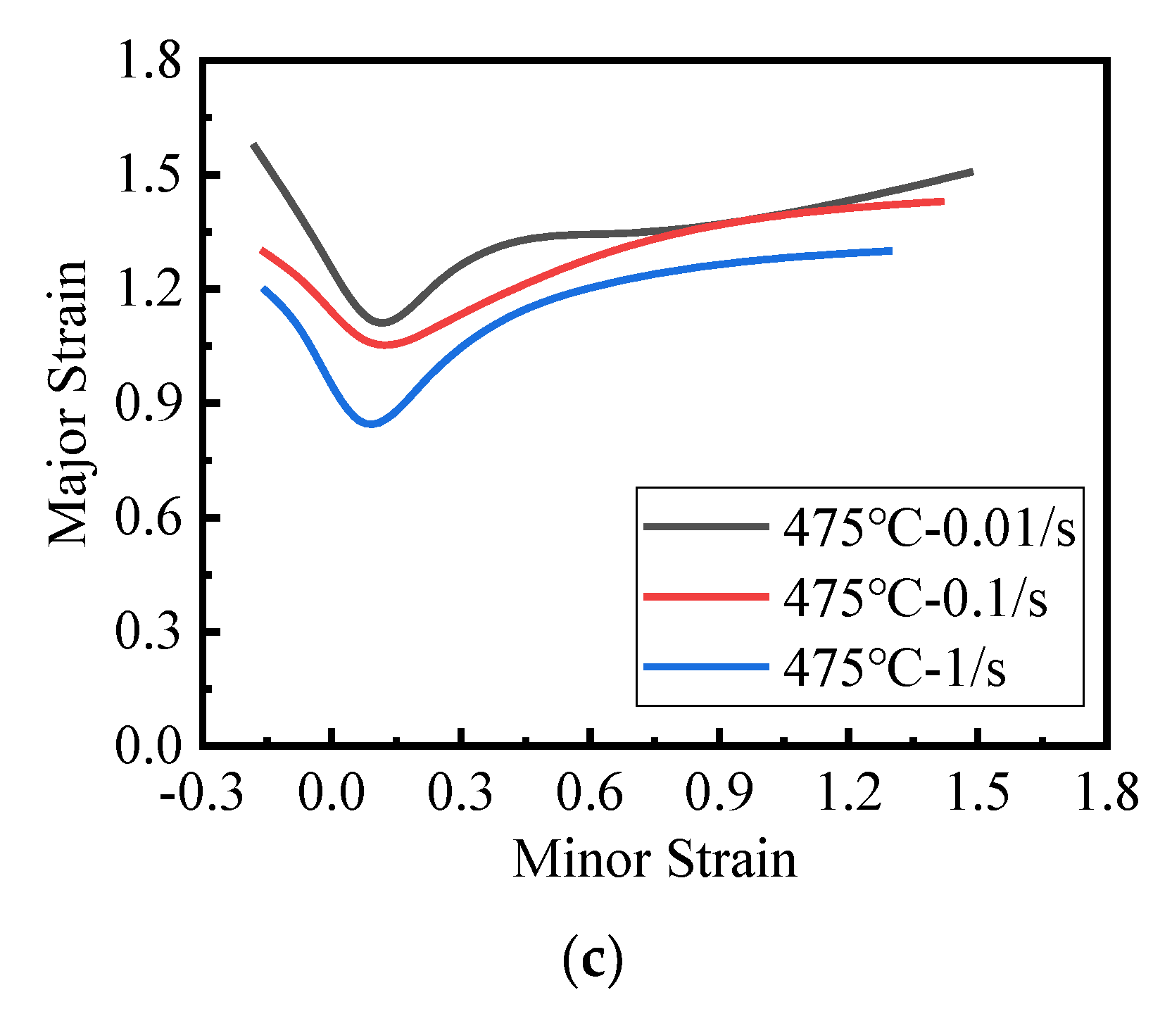
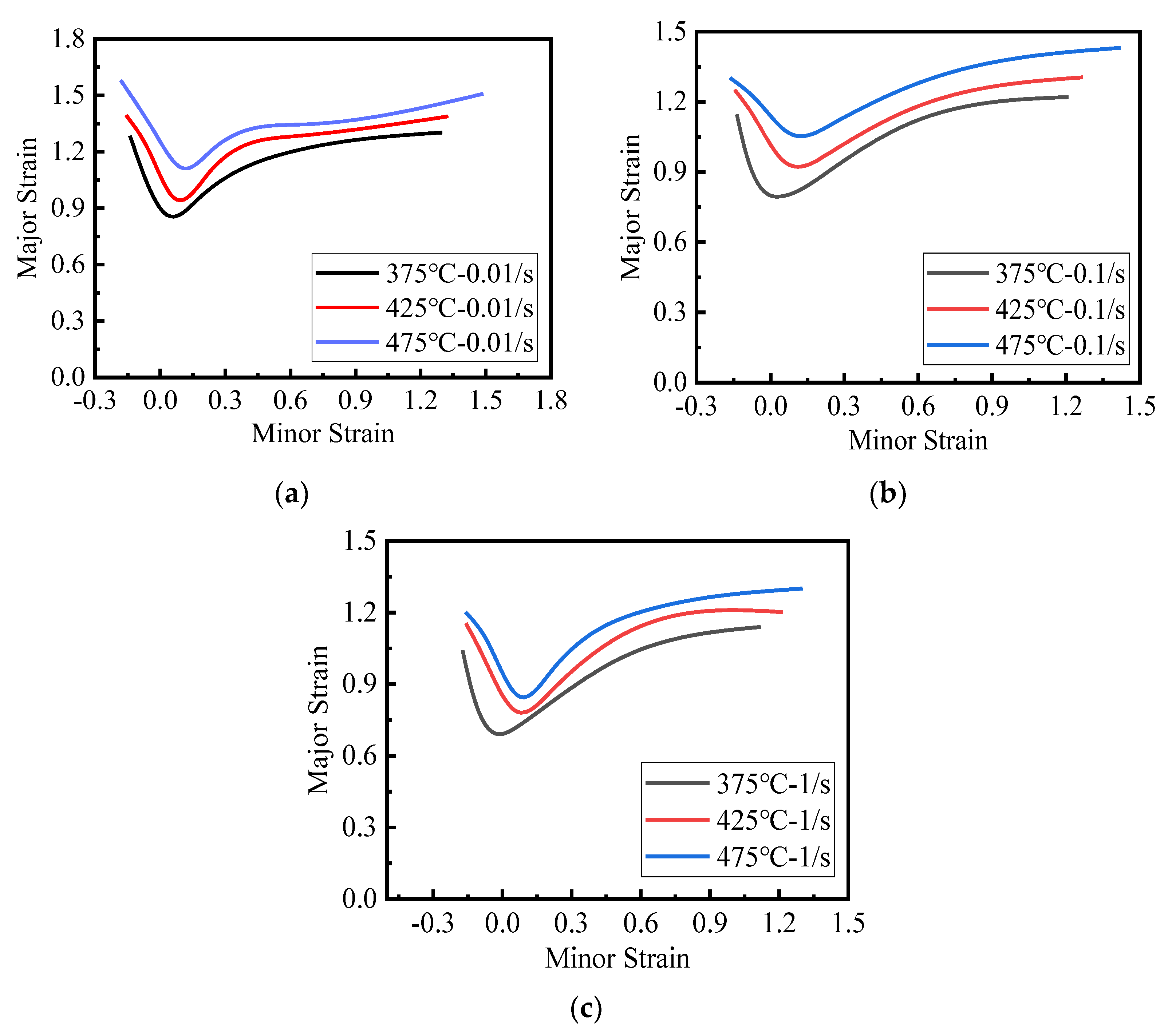
5.1. Theoretical Forming Limit Curve

Obtaining the forming limit curve by the high-temperature Nakazima test has many uncertainty factors, such as time node, temperature control, and lubrication conditions, and these factors affect each other. Therefore, a large number of repeated tests are needed, which puts forward higher requirements for test equipment and the working environment. Consequently, the test difficulty and cost increase significantly. Therefore, based on the high-temperature bulging test method, this study used FEM simulation analysis to draw the theoretical forming limit curve under different conditions.

The finite element simulation model of the Nakazima test was constructed using ABAQUS software. The punch size was 90 mm, the die size was 130 mm, and the die fillet was 5 mm. C3D8R mesh type was used for mesh division, the mesh size of the specimen was set to 1 mm, and shell elements were used in both mold tools and specimens. Surface-to-surface contact was selected between the die and the specimen, and the friction coefficient was set to 0.1. Surface-to-surface contact was also selected between the hemisphere punch and the specimen, and the friction coefficient was set to 0.001. The function of the blank holder is set to apply a fully fixed constraint on the side of the specimen. The relative position of each part is shown in Figure 20a. To obtain the principal strain under different strain paths, five different widths of bone-shaped and circular plate specimens were selected according to the China national standard GB/T 24171-2009. The total diameter of each specimen is 180 mm. Figure 20b shows the shape of the selected bone-shaped specimen. The length of the parallel segment L is 90 mm, the radius of the transition arc is 20 mm, and the width dimensions are listed in

Table 4. Width specification of a bone-shaped specimen.

Type Number	W20	W40	W60	W80	W100
Width (mm)	20	40	60	80	100

.

The failure of the material is determined according to the accumulation value of the damage factor $\xi$. When the damage factor $\xi$ accumulates from 0 to 1, the material is considered to have completely failed. According to the calculation, when the damage variable of the material is between 0.8 and 1, fracture failure has already occurred [27,28]. Figure 21 describes the damage distribution of different samples in the frame before rupture when the temperature is 375 °C and the strain rate is 0.01/s. Sample W20 is close to the unidirectional tensile state, and the fracture starts at the geometric center of the specimen, which is similar to the actual fracture state. The cracks in the other four bone samples also spread from the middle to both sides, and the circular plate samples break from the top of the punch and spread around. The damaged fracture locations under other conditions were the same as those at 375 °C.

Two principal strains in the plane of specimens with different shapes and specifications under certain temperature and strain rate conditions were extracted, and the theoretical forming limit curve was obtained, as shown in Figure 22 and Figure 23. Based on the constructed Johnson–Cook fracture model, the theoretical forming limit curve of AA7075 aluminum alloy can be predicted. Such a prediction avoids the influence of experimental uncertainty factors, saves manpower and time, and plays an important auxiliary role in studying the hot-forming performance of the 7075 aluminum alloy.

It can be seen from Figure 22 and Figure 23 that the theoretical forming limit of AA7075 aluminum alloy decreases with an increasing strain rate at a constant temperature. In contrast, under the same strain rate, the theoretical forming limit of AA7075 aluminum alloy gradually increases with increasing temperature.

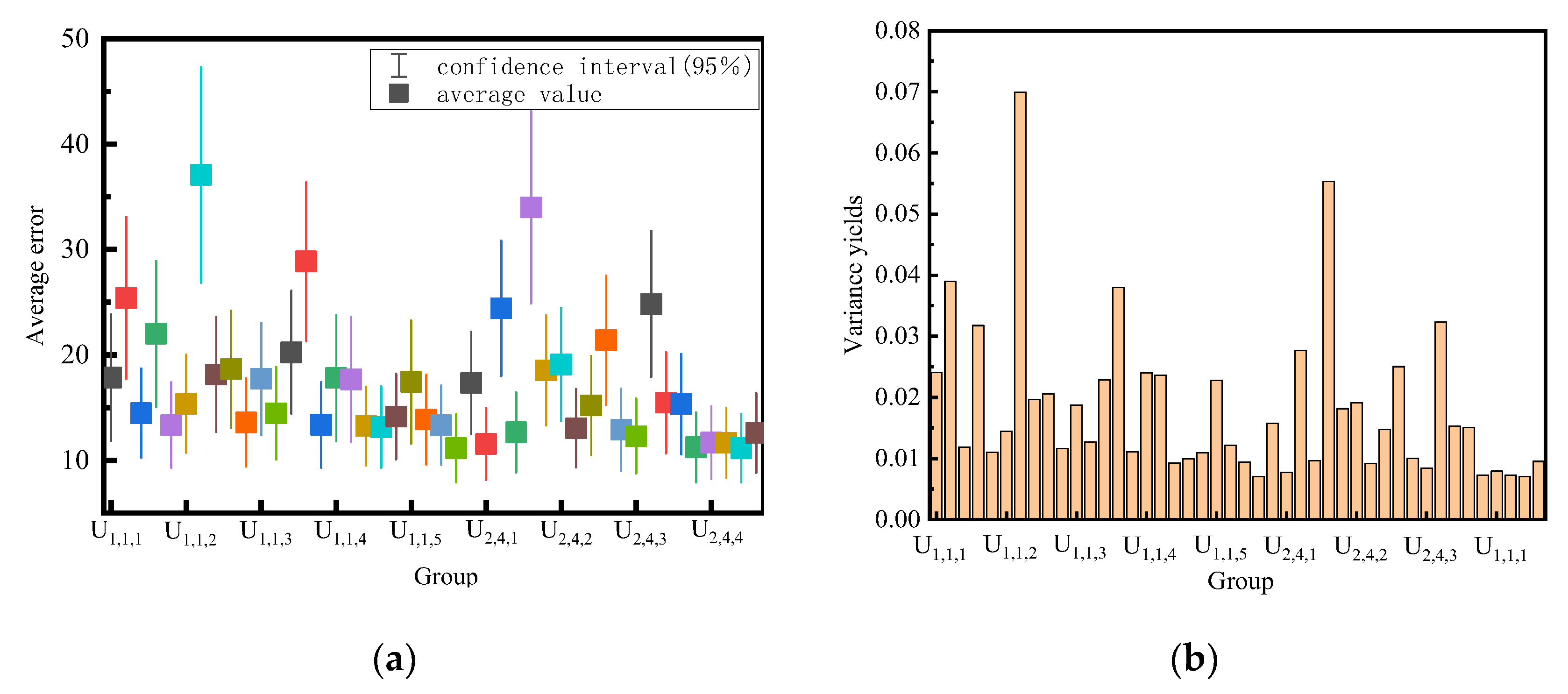
5.2. Prediction Accuracy Assessment

To verify the accuracy of the Johnson–Cook fracture model and theoretical forming limit curve, a high-temperature bulging test was conducted. In the high-temperature Nakazima test, an INSPEKT Table 100 kN electronic universal high-temperature testing machine was used to control the temperature and binder force of the hot stamping device as bulging equipment. The punch diameter of the hot-stamping device was 20 mm, and the inner circle diameter of the die was 30 mm. The schematic diagram is shown in Figure 24.

According to the test procedure, bulging tests of circular plates with strain rates of 0.01, 0.1, and 1/s were completed at a forming temperature of 375 °C. A physical diagram of the bulging fracture is shown in Figure 25.

Based on ABAQUS software, a finite element simulation model was constructed. The material properties were constitutive parameters under the same conditions when uniaxial tension was applied. The friction coefficient between the punch and the mold was set to 0.2. The damage and fracture cloud map before the fracture was extracted. By analyzing the data of the fracture position and displacement in the simulation results, the accuracy of the prediction model was evaluated by comparing it with the experimental values.

Figure 26 shows a comparison between the predicted fracture position of the circular plate specimen based on the Johnson–Cook fracture model and the test results. The test and simulated fracture positions are close, and both break from the edge of the top circular area.

Figure 27 shows the fracture displacement of the circular plate specimen predicted using the Johnson–Cook fracture model. At 375 °C and 0.01/s, the experimental value of the fracture displacement is 16.924 mm, the simulated fracture displacement is 16.41 mm, and the relative error is 3%. At 375 °C and 0.1/s, the experimental value of the fracture displacement is 16.18 mm, the simulated fracture displacement is 16.06 mm, and the relative error is 0.7%. At 375 °C and 1/s, the experimental value of the fracture displacement is 15.67 mm, the simulated fracture displacement is 15.36 mm, and the relative error is 2%. The simulated fracture displacement is less than the experimental fracture displacement, which increases the safety margin, and the relative error can be controlled within 5%. The aforementioned results show that the prediction accuracy of circular plate bulging based on the Johnson–Cook fracture model simulation prediction is high, which confirms the high accuracy of the obtained theoretical forming limit curve.

6. Conclusions

(1)

The Johnson–Cook constitutive model was constructed and modified based on the high-temperature uniaxial tensile test of AA7075 aluminum alloy. The modified Johnson–Cook constitutive model has good applicability by modifying the Holloman hardening model to the Swift–Voce hardening model.

(2)

After the Johnson–Cook fracture model of AA7075 aluminum alloy was constructed, error evaluation was conducted based on 44 combination schemes calibrated by the model. The optimal combination scheme of specimens and optimal values of five failure parameters were determined. Based on the Johnson–Cook fracture model, the theoretical forming limit curves were obtained for different strain rates and temperatures.

(3)

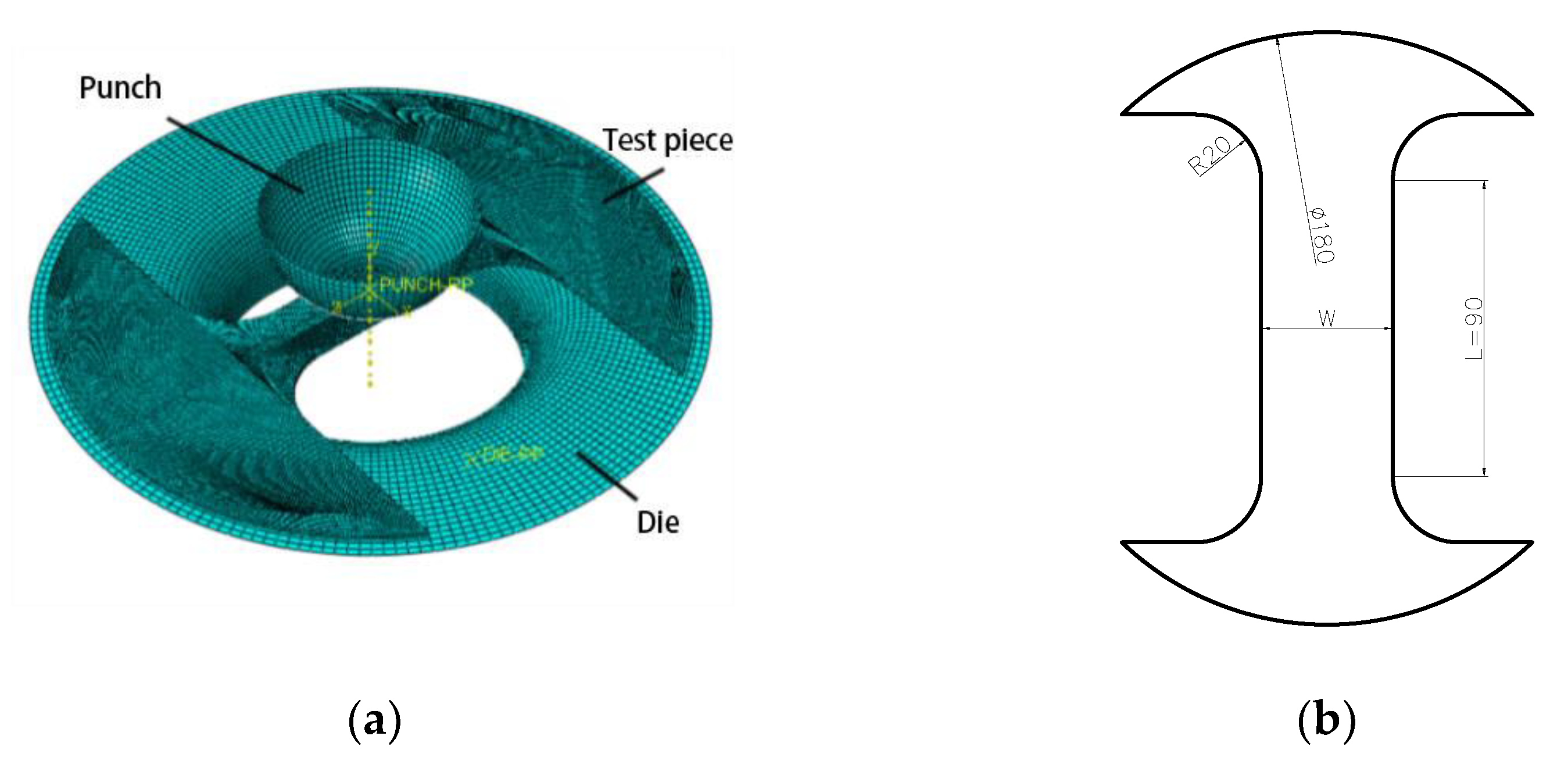
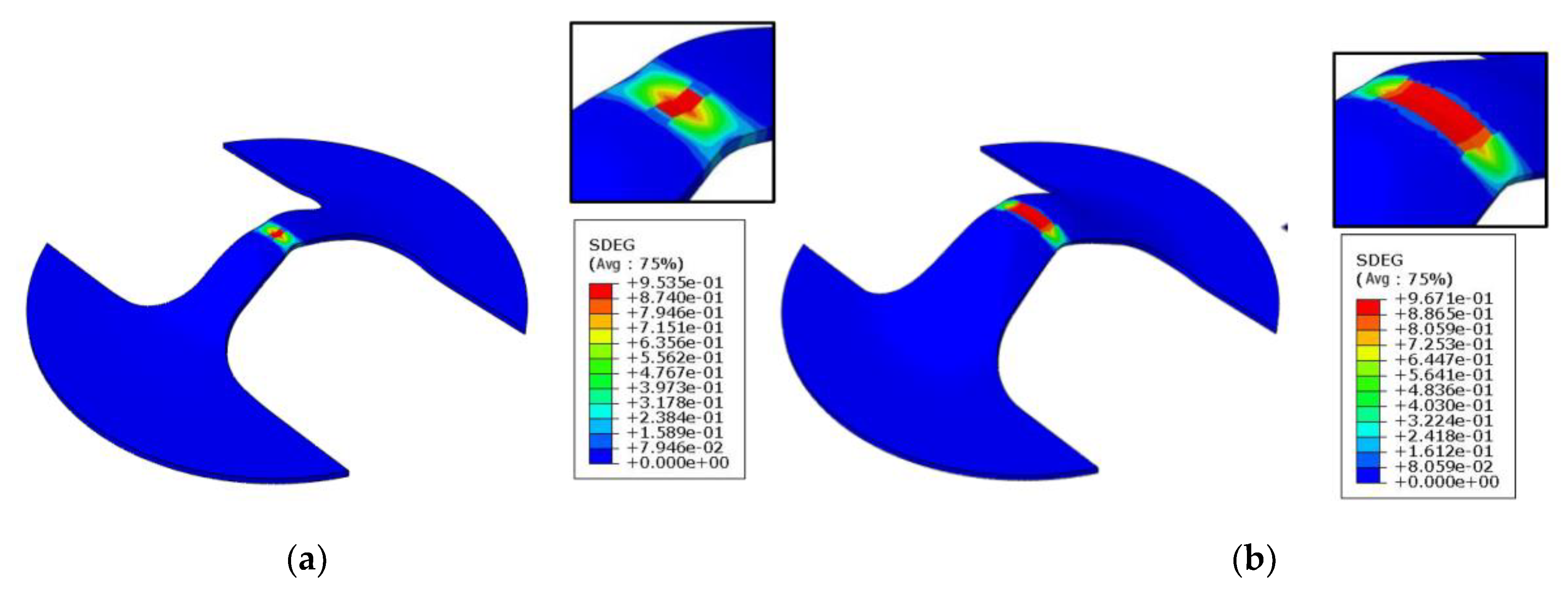
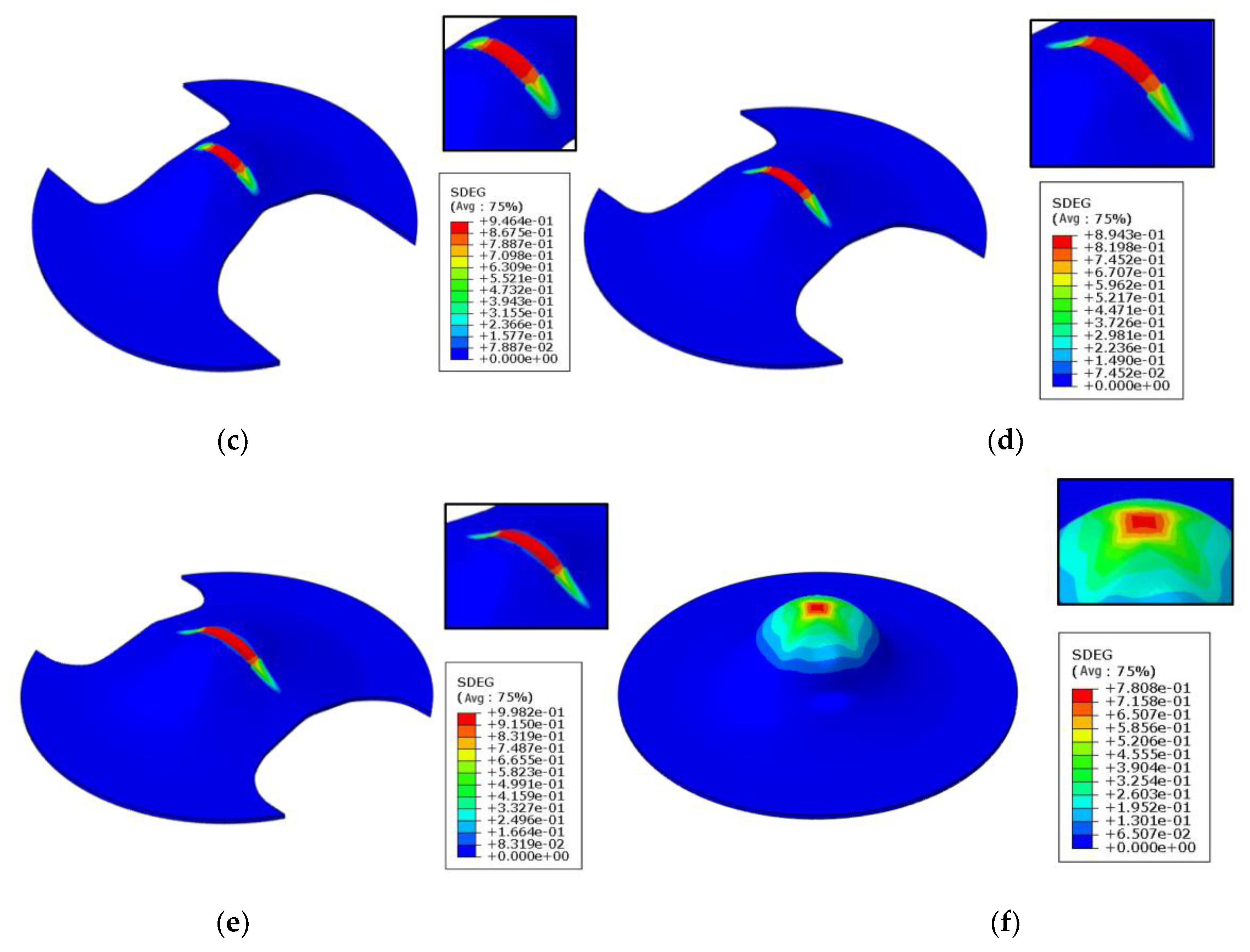
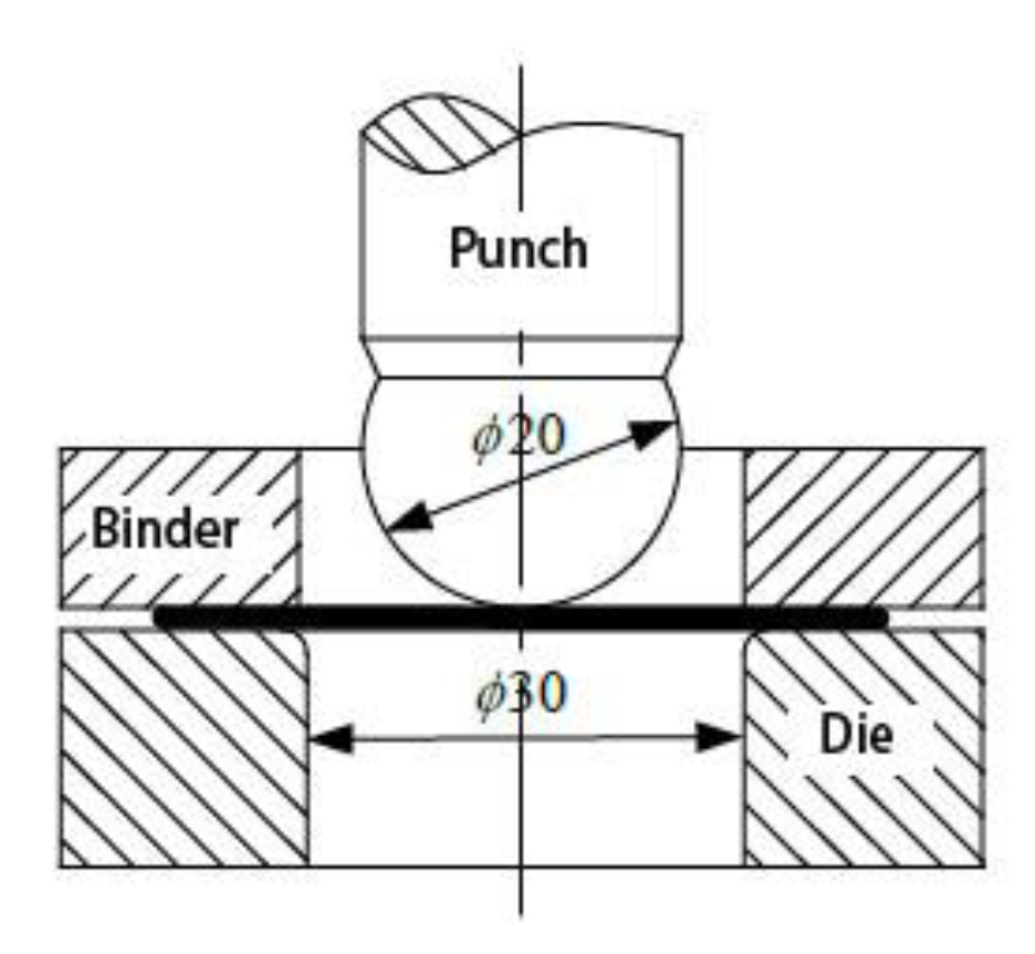
The reliability of the Johnson–Cook fracture model was predicted and evaluated through a Nakazima test of an AA7075 aluminum alloy circular plate. The experimental fracture location was in good agreement with the simulated fracture location, and the fracture displacement error was controlled within 5%. The results show that the prediction accuracy of circular-plate bulging based on the Johnson–Cook fracture model simulation prediction is high, which confirms the high accuracy of the obtained theoretical forming limit curve.

References

1. Andilab, B.; Vandersluis, E.; Emadi, P.; Ravindran, C.; Byczynski, G.; Fernandez-Gutierrez, R. Characterization of a cast Al-Cu alloy for automotive cylinder head applications. J. Mater. Eng. Perform. 2022, 31, 5679–5688. [Google Scholar] [CrossRef]
2. Wojdat, T.; Kustron, P.; Jaskiewicz, K.; Zwierzchowski, M.; Margielewska, A. Numerical modelling of welding of car body sheets made of selected aluminium alloys. Arch. Metall. Mater. 2019, 64, 1403–1409. [Google Scholar]
3. Wu, B.T.; Pan, Z.X.; Ziping, Y.; van Duin, S.; Li, H.J.; Pierson, E. Robotic skeleton arc additive manufacturing of aluminium alloy. Int. J. Adv. Manuf. Technol. 2021, 114, 2945–2959. [Google Scholar] [CrossRef]
4. Kablov, E.N.; Antipov, V.V.; Oglodkova, J.S.; Oglodkov, M.S. Development and application prospects of aluminum-lithium alloys in aircraft and space technology. Metallurgist 2021, 65, 72–81. [Google Scholar] [CrossRef]
5. Wang, X.J.; Sun, W.; Chen, J.F.; Wang, F.Y.; Li, L.; Cui, J.Z. Microstructures and properties of 6016 aluminum alloy with gradient composition. Rare Met. 2021, 40, 2154–2159. [Google Scholar] [CrossRef]
6. Kenevisi, M.S.; Yu, Y.F.; Lin, F. A review on additive manufacturing of Al-Cu (2xxx) aluminium alloys, processes and defects. Mater. Sci. Technol. 2021, 37, 805–829. [Google Scholar] [CrossRef]
7. Liu, W.; Zou, X.F.; Lei, Y. Improving shape accuracy of aluminium alloy surface part in electromagnetically-assisted stamping. Int. J. Mater. Prod. Technol. 2020, 60, 260–273. [Google Scholar] [CrossRef]
8. Ponnusamy, P.; Rashid, R.A.R.; Masood, S.H.; Ruan, D.; Palanisamy, S. Mechanical properties of SLM-Printed aluminium alloys: A review. Materials 2020, 13, 4301. [Google Scholar] [CrossRef]
9. Simonetto, E.; Bertolini, R.; Ghiotti, A.; Bruschi, S. Mechanical and microstructural behaviour of 7075-T6 aluminium alloy for sub-zero temperature sheet stamping process. Int. J. Mech. Sci. 2020, 187, 105919. [Google Scholar] [CrossRef]
10. Gao, H.X.; El Fakir, O.; Wang, L.L.; Politis, D.J.; Li, Z.Q. Forming limit prediction for hot stamping processes featuring non-isothermal and complex loading conditions. Int. J. Mech. Sci. 2017, 131, 792–810. [Google Scholar] [CrossRef]
11. Mallick, P.K.; Sheng, Z.Q. Predicting sheet forming limit of aluminum alloys for cold and warm forming by developing a ductile failure criterion. J. Manuf. Sci. E-T. ASME 2017, 139, 111018. [Google Scholar]
12. Zhan, X.P.; Wang, Z.H.; Li, M.; Hu, Q.; Chen, J. Investigations on failure-to-fracture mechanism and prediction of forming limit for aluminum alloy incremental forming process. J. Mater. Process. Technol. 2020, 282, 116687. [Google Scholar] [CrossRef]
13. Chakrabarty, S.; Bhargava, M.; Narula, H.K.; Pant, P.; Mishra, S.K. Prediction of strain path and forming limit curve of AHSS by incorporating microstructure evolution. Int. J. Adv. Manuf. Technol. 2020, 106, 5085–5098. [Google Scholar] [CrossRef]
14. Yang, Z.Y.; Zhao, C.C.; Dong, G.J.; Chen, Z.W. Experimental Calibration of ductile fracture parameters and forming limit of AA7075-T6 sheet. J. Mater. Process. Technol. 2021, 291, 117044. [Google Scholar] [CrossRef]
15. Morchhale, A.; Badrish, A.; Kotkunde, N.; Singh, S.K.; Khanna, N.; Saxena, A.; Nikhare, C. Prediction of fracture limits of Ni-Cr based alloy under warm forming condition using ductile damage models and numerical method. Trans. Nonferrous Met. Soc. China 2021, 31, 2372–2387. [Google Scholar] [CrossRef]
16. Goksen, S.; Darendeliler, H. The Effect of Strain Rate and Temperature on Forming Limit Diagram for DKP-6112 and AZ31 Materials. In Proceedings of the 23rd International Conference on Material Forming, online, 4–8 May 2020. [Google Scholar]
17. Nasri, M.T.; Abbassi, F.; Ahmad, F.; Makhloufi, W.; Ayadi, M.; Mehboob, H.; Choi, H.S. Experimental and numerical investigation of sheet metal failure based on Johnson-Cook model and Erichsen test over a wide range of temperatures. Mech. Adv. Mater. Struct. 2022. [Google Scholar] [CrossRef]
18. Hidalgo-Manrique, P.; Cao, S.; Shercliff, H.R.; Hunt, R.D.; Robson, J.D. Microstructure and properties of aluminium alloy 6082 formed by the hot form quench process. Mater. Sci. Eng. A 2021, 804, 140751. [Google Scholar] [CrossRef]
19. Barenji, A.B.; Eivani, A.R.; Hasheminiasari, M.; Jafarian, H.R.; Park, N. Effects of hot forming cold die quenching and inter-pass solution treatment on the evolution of microstructure and mechanical properties of AA2024 aluminum alloy after equal channel angular pressing. J. Mater. Res. Technol. 2020, 9, 1683–1697. [Google Scholar] [CrossRef]
20. Garrett, R.P.; Lin, J.; Dean, T.A. An Investigation of the effects of solution heat treatment on mechanical properties for AA 6xxx alloys: Experimentation and modelling. Int. J. Plast. 2005, 21, 1640–1657. [Google Scholar] [CrossRef]
21. Dunand, M.; Mohr, D. Hybrid experimental–numerical analysis of basic ductile fracture experiments for sheet metals. Int. J. Solids Struct. 2010, 47, 1130–1143. [Google Scholar] [CrossRef]
22. Johnson, G.R.; Cook, W.H. Fracture characteristics of three metals subjected to various strains, strain rates, temperatures and pressure. Eng. Fract. Mech. 1985, 21, 31–48. [Google Scholar] [CrossRef]
23. Jia, Z.; Guan, B.; Zang, Y.; Wang, Y.; Mu, L. Modified Johnson-Cook model of aluminum alloy 6016-T6 sheets at low dynamic strain rates. Mater. Sci. Eng. A 2021, 820, 141565. [Google Scholar] [CrossRef]
24. Wang, C.J.; Wang, H.Y.; Chen, G.; Zhu, Q.; Zhang, P.; Fu, M.W. Experiment and modeling based studies of the mesoscaled deformation and forming limit of Cu/Ni clad foils using a newly developed damage model. Int. J. Plast. 2022, 149, 103173. [Google Scholar] [CrossRef]
25. Yao, D.; Pu, S.L.; Li, M.Y.; Guan, Y.P.; Duan, Y.C. Parameter identification method of the semi-coupled fracture model for 6061 aluminium alloy sheet based on machine learning assistance. Int. J. Solids Struct. 2022, 254, 111823. [Google Scholar] [CrossRef]
26. Ganjiani, M.; Homayounfard, M. Development of a ductile failure model sensitive to stress triaxiality and Lode angle. Int. J. Solids Struct. 2021, 225, 111066. [Google Scholar] [CrossRef]
27. Abbassi, F.; Belhadj, T.; Mistou, S.; Zghal, A. Parameter identification of a mechanical ductile damage using Artificial Neural Networks in sheet metal forming. Mater. Des. 2013, 45, 605–615. [Google Scholar] [CrossRef] [Green Version]
28. Abbassi, F.; Mistou, S.; Zghal, A. Failure analysis based on microvoid growth for sheet metal during uniaxial and biaxial tensile tests. Mater. Des. 2013, 49, 638–646. [Google Scholar] [CrossRef] [Green Version]
Figure 1. Shape and size of the applied specimens (the dimensions are in mm).
Metals 13 00231 g001
Figure 2. HFQ hot forming process route map.
Metals 13 00231 g002
Figure 3. Hot tensile test system.
Metals 13 00231 g003
Figure 4. Tensile force—displacement curve of UT specimen under a certain strain rate. (a) 0.01/s; (b) 0.1/s; and (c) 1/s.
Metals 13 00231 g004aMetals 13 00231 g004b
Figure 5. Force—displacement curves of NT2.5 specimens at (a) 0.1/s and (b) 425 °C.
Metals 13 00231 g005
Figure 6. Force—displacement curves of NT5 specimens at (a) 0.1/s and (b) 425 °C.
Metals 13 00231 g006
Figure 7. Force—displacement curves of NT10 specimens at (a) 0.1/s and (b) 425 °C.
Metals 13 00231 g007
Figure 8. Force—displacement curves of SH specimens at (a) 0.1/s and (b) 425 °C.
Metals 13 00231 g008
Figure 9. Comparison of the constitutive fitting curves and test curves at different strain rates. (a) 0.01/s; (b) 0.1/s; and (c) 1/s.
Metals 13 00231 g009
Figure 10. Finite element geometric model of the studied specimens. (a) UT; (b) NT2.5; (c) NT5; (d) NT10; and (e) SH.
Metals 13 00231 g010
Figure 11. Experimental failure image and FEM results of the specimen fracture initiation moment. (a) UT; (b) NT2.5; (c) NT5; (d) NT10; and (e) SH.
Metals 13 00231 g011aMetals 13 00231 g011b
Figure 12. Evolution process of stress triaxiality at the fracture critical point of UT specimen. (a) 375 °C; (b) 425 °C; and (c) 475 °C.
Metals 13 00231 g012aMetals 13 00231 g012b
Figure 13. Evolution process of stress triaxiality at the fracture critical point of N2.5 specimen. (a) 0.1/s and (b) 425 °C.
Metals 13 00231 g013
Figure 14. Evolution process of stress triaxiality at the fracture critical point of NT5 specimen. (a) 0.1/s and (b) 425 °C.
Metals 13 00231 g014
Figure 15. Evolution of stress triaxiality at the fracture critical point of NT10 specimen. (a) 0.1/s and (b) 425 °C.
Metals 13 00231 g015
Figure 16. Evolution of stress triaxiality at the fracture critical point of SH specimen. (a) 0.1/s and (b) 425 °C.
Metals 13 00231 g016
Figure 17. Johnson–Cook fracture model failure parameter fitting.
Metals 13 00231 g017
Figure 18. D4 and D5 failure parameter distribution.
Metals 13 00231 g018
Figure 19. Theoretical prediction of the error mean and variance of fracture strain. (a) δ a v g and (b) s 2 .
Metals 13 00231 g019
Figure 20. Finite element simulation model of the Nakazima test and specimen specification shape. (a) Finite element simulation model of the Nakazima test and (b) specimen specification shape.
Metals 13 00231 g020
Figure 21. Damage distribution of the frame before fracture under certain conditions (375 °C, 0.01 s−1). (a) W 20. (b) W 40. (c) W 60. (d) W 80. (e) W 100. (f) circular plate.
Metals 13 00231 g021aMetals 13 00231 g021b
Figure 22. Theoretical forming limit curves at the same temperature and different strain rates. (a) 375 °C; (b) 425 °C; and (c) 475 °C.
Metals 13 00231 g022aMetals 13 00231 g022b
Figure 23. Theoretical forming limit curves at the same strain rate and different temperatures. (a) 0.01/s; (b) 0.1/s; and (c) 1/s.
Metals 13 00231 g023
Figure 24. High-temperature bulging test work schematic diagram.
Metals 13 00231 g024
Figure 25. Specimen after bulging fracture. (a) 375 °C—0.01/s; (b) 375 °C—0.1/s; and (c) 375 °C—1/s.
Metals 13 00231 g025
Figure 26. Johnson–Cook comparison of the predicted fracture position of a specimen based on the fracture model simulation and the test results. (a) 375 °C—0.01/s; (b) 375 °C—0.1/s; and (c) 375 °C—1/s.
Metals 13 00231 g026
Figure 27. Simulation results of the fracture displacement of a circular-plate specimen. (a) 375 °C, 0.01/s; (b) 375 °C, 0.1/s; and (c) 375 °C, 1/s.
Metals 13 00231 g027