Transient Strain Monitoring of Weldments Using Distributed Fiber Optic System

Abstract

The primary objective of this study was to evaluate the capability of a distributed fiber optic sensor to capture in situ dynamic transient strain formation during and post-weldment on the surface of a steel plate. The study involved a vertical manual weld of a bead on a plate on a 300 mm × 300 mm × 6.35 mm A36 steel plate (European equivalent S235J2; Chinese equivalent Q235B) clamped at the corners. A fiber optic distributed sensor was used to measure the surface total and thermal strains on the welded side of the plate adjacent to the weld path. Experimental results show a complex behavior of strain changes during the welding process and the residual strain formation post-welding. This study aims to document the use of distributed fiber optic sensing techniques in welding applications. Validations of the experimental data were performed using VrWeld, a commercial software framework for computational weld mechanics, and an iPhone FLIR One Pro. thermographic camera. The experimental results demonstrated that although distributed fiber optic sensing based on Rayleigh backscattering is an appropriate and useful technique for total strain measurements, the manufacturing and the materials used for the thermal sensors are critical in obtaining optimal results. Finally, this study highlights the challenges encountered in synchronizing large experimental data sets captured with different instruments with computational welding mechanic (CWM) models.

1. Introduction

Welding has become an essential process in many industries, such as the construction and automotive industries. The increased need for a physics-based understanding of the structural integrity of welded joints has resulted in an in-depth look at the formation of residual stresses (RS) during arc welding processes. The uneven temperature distribution of manual weldments, high thermal strains, and microstructure changes produced during welding can lead to the formation of RS along the welded joint. This, in turn, affects the mechanical performance of the joint, thus highlighting the need to optimize these effects. These may include fluctuating stresses being applied during the operational service of the joint. The integration of plastic strain rates during welding leads to a residual strain field that generates RS in the weldment, thus affecting the durability of the joint [1]. The use of in situ sensors capable of accurately measuring the real-time total and thermal strain during the welding process may provide industry partners with an understanding of the transient strain formation which is known to affect the microstructure of the material [2]. In this study, the primary focus is the use of novel instrumentation techniques and how they help in the validation process of transient computational welding mechanic (CWM) models, versus the actual physics that leads to the formation of RS or microstructural changes within the weldment. In addition, this study attempts to document the challenges of big data synchronization with respect to CWM models.

In many industries and academic studies, the use of experimental mechanics techniques such as Digital Image Correlation (DIC) [3], Fiber Optic Systems (FOS) [4], and foil Strain Gauges (SG) have often been used for the measurement of strains [5]. However, as documented in the open literature, each one of these sensing systems has advantages and disadvantages when applied to weldments. In the welding of metallic structures, the evaluation of strain distribution using DIC is not a trivial matter. In part, this is due to the high-intensity light emitted during the welding process, saturating the digital cameras commonly utilized. Strycker et al. used DIC for measuring welding deformation due to thermal strains in a tubular structure. A speckle pattern was applied to the side of the pipe, while the welding was performed on the upper section of the pipe. The authors were able to obtain good agreement between their DIC thermal strain fields in relation to strain gauges. This allowed the authors to validate their FEM over a large region of their structure [6]. In [7], the authors were able to measure the dynamic strain formation at the back of a welded plate. However, the authors did not make use of any optical and/or filtering techniques to suppress the light emission experienced during welding, and thus they were unable to capture the strain formation at the front of the plate. Other researchers have successfully been able to make use of DIC in welding studies through the application of optical illumination and filtering techniques as documented in [8]. C. Hageloncher et al. in [9] made use of photogrammetry and DIC with a very good temporal and spatial resolution to determine the compressive and tensile strain regions in the proximity of the weld path. In their study, they were able to show and determine the thermomechanical response of the material during welding. They also documented how the tensile and compressive strain regions led to centerline cracks in their application. In this study, we attempt to document our progress on how to measure total strain and thermal strain along a fiber on the front side of the weld using distributed sensing FOS.

FOS have been considered as a potential replacement to foil SG, the latter is known to be susceptible to Electro-Magnetic Interference (EMI) [10]. In addition, SG are only able to capture very small regions of the complex strain field under study. Within the field of fiber optic technology, Fiber Bragg Gratings (FBGs) and their predecessors Fabry-Perot are considered discrete measurement systems which are only able to provide a strain measurement at the location of the gratings or discontinuity in the fiber [11]. Newer FBG systems can apply many gratings along the fiber length with a high data acquisition rate; however, this makes the sensor more expensive. In weldments, the use of FBGs to monitor the welding of steel plates has been reported by Rodriguez-Cobo et al. in [12]. The authors documented the use of FBGs to measure the plasma radiation in addition to the thermal and mechanical strains on the TIG welding of two AISI-304 plates. The authors embedded the FBG inside a plastic film to increase the sensitivity of the FBG sensor to the acoustic waves generated during the welding process. The acoustic wave required the system to gather the data at an acquisition rate of 10 kHz. The FBGs adhered to the plate were able to capture the deformation of the plates, while a floating orthogonal FBG was placed at an angle facing the approaching arc. The authors documented the ability of the floating FBG to capture the changes in the temperature and air pressure in the air surrounding the arc during the welding process. The experimental results showed a good correlation with the plasma spectroscopy approach. Other studies have implemented a limited number of FBGs to measure strain at discrete points. For example, Suarez et al. in [13] looked at transient strain formation for a TIG weld in comparison to thermocouples located on an Al-Mg test plate. Spatially distributed FOS were also used by Petrie et al. looking at phase transformations and RS evolution for the selection of low-transformation-temperature filler metals in high-strength steel welding [14]. Recently, K. Schricker et al. in [15] evaluated the use of FBG sensors for monitoring laser-assisted metal-polymer joints. The authors were able to understand the effect of clamping forces between the metal and a polymer substrate, which is critical for the welding of overlap joints. The authors made use of polypropylene and polyamide-coated fibers and clearly describe the difference between the two fiber types. In addition, the authors clearly state the need for temperature compensation using thinner FBG in combination with numerical models and the required use of process simulations of welding processes, including residual strain determination.

A second generation of optical sensing systems based on Raman [16], Brillouin [17], or Rayleigh backscattering has entered the market [18]. These are known as Fiber Optic Distributed Sensing Systems (FODSS), which are different from discrete FBG-based systems and can provide thousands of data points along a fiber optic line. These systems have the capability of capturing a data point (total and/or thermal strain) at every millimeter along the length of a commercial fiber optic line without the need for gratings. In FODSS, strain is measured as a change in the backscattering signal of different wavelengths due to the interactions between light photons traveling inside the fiber core. As each fiber has an inherent material microstructure, this interaction of the light photons is unique for each fiber section. As such, a baseline signal of the backscattering signal is recorded in a non-strained state. As the fiber is stretched either due to a thermal or mechanical strain, the backscattering signal changes proportionally to the applied strain at every millimeter along the fiber length. The baseline non-strained state backscattering signal is compared to the strained state through a cross-correlation function. This comparison provides measurement of the change in strain at each section of the fiber in time. Martinez-Bueno et al. made use of Rayleigh backscattering technology to instrument and validate a Finite Element Model (FEM) of a composite wing of an Unmanned Aerial Vehicle (UAV) [19]. In [20], Baldassarre et al. demonstrated the accuracy of the FODSS with respect to discrete single-point measurements such as strain gauges and surface strain measurement technology such as DIC. The author concluded that for anisotropic materials, surface strain measurements such as DIC showed that they were more accurate than a single point or line measurement technique. The authors recommended that, even though ASTM standards for material characterization highlight the use of strain gauges, more accurate material properties could be achieved using FODSS or DIC.

In situ monitoring of the welding process is still an unresolved challenge despite the advancement of discrete sensing systems with high data acquisition rates. Non-contact systems such as DIC and thermography require a field of view which is not always available. An experimental validation study on the use of distributed FOS in the proximity of the weld pool (WP) has not been documented in the literature. A primary objective of this study was to evaluate their use for in-service field application. A secondary objective was to evaluate the use of FOS to validate a CWM model of the welding process while documenting the challenges encountered in the synchronization of big data between the experimental results and the CWM results. It is hypothesized that the use of FOS may provide the welding community with the ability to understand strain formation and its complex dynamic behavior during arc welding in an operational manufacturing environment.

2. Methodology

2.1. Experimental Setup

Experiments were conducted at Clarkson University’s welding laboratory. A bead-on-plate weld was performed on a 300 mm × 300 mm × 6.35 mm A36 steel plate (European equivalent S235J2; Chinese equivalent Q235B), as shown in Figure 1. The welding lab is equipped with a Miller 350 power supply connected to a TIG welder. A 20 cm bead on plate manually performed at an average speed of 2 mm/s was executed by a professional welder. The power supply was set to an average voltage of 13.7 Volts, while the current was varied by the welder as the bead on plate was being performed. The average power for the 100 s weld was approximately 2500 Watts. It is important to emphasize that to assist in the computational welding mechanics (CWM) model validation and synchronization of the data, the use of fiducial markers was essential. The fiducial markers consisted of 6.35 mm holes randomly distributed but with known locations throughout the height of the plate, as shown in Figure 1. The introduction of fiducial markers was extremely helpful in determining the location of the WP at every instant in time during welding. One of the primary challenges in setting up this study was the synchronization of the data captured from the different measurement systems. This challenge was overcome through (i) the use of fiducial markers to determine the position of the WP along its path; (ii) the use of a stopwatch to determine the start time of two independent DAQ systems (cameras and LUNA fiber optic system); and (iii) the use of the same DAQ acquisition rates across all instruments. This served the authors well when synching the experimental findings with those of the VrWeld FEM. Previous attempts had been performed without fiducial markers, creating a major challenge in synching experimental and FEM results. The stochastic nature of a manual weld adds an extra layer of complexity in synchronizing computational and experimental data sets.

The plate once instrumented with the optical distributed fiber was C-clamped at the four corners to a test fixture. The test fixture was also clamped to the table to ensure no movement during the experiment, as shown in Figure 1. As seen in Figure 1A, cloth strips and aluminum tape were applied on either side of the weld path to protect exposed parts of the fiber optic sensor during the weld. Previous attempts had shown that leaving the fiber exposed could cause it to burn from arc sputters. Figure 1B shows a schematic of the optical fiber layout and the different segments of the fiber sensor.

The LUNA FOS is very sensitive to temperature changes, as soon as the arc strikes the plate, a peak in the thermal strain field is captured. A stopwatch was used to determine a time offset to compare with the VrWeld computer model that starts at zero seconds. The placement of the bead with respect to the edges, through the burn, size of the weld bead, and average speed of the weld is provided to the computational weld mechanics (CWM) team for them to use as input into their model. The data acquisition rate of the LUNA FOS was set to 1 Hz.

Monochrome 2.3-megapixel Grasshopper 3 cameras were positioned to capture the current and voltage supplied by the welding power supply digital readout [21]. This information allowed the CWM team to determine the moving average power used at any moment in time during welding. It is well understood by the authors that the digital readout’s actual power is not the same as that which is supplied to the welding arc. However, it does provide an estimate of the average power supplied over time. An additional camera was used to capture the light emitted from the arc and set at a data acquisition rate of 1 Hz (same as all other DAQ systems). This second camera serves to inform the team of the duration of the weld and synchronize with the power data. A fan was placed on the back of the specimen. The fan was used to cool one side of the plate. It was primarily intended to assist in maintaining a flow of air on the back of the plate. This is critical for achieving cross-correlation with the DIC system. It is known that heat build-up of the air between the cameras and the surface being studied can affect the results of the DIC system. The authors of this study are also aware that this would affect the residual strain formation.

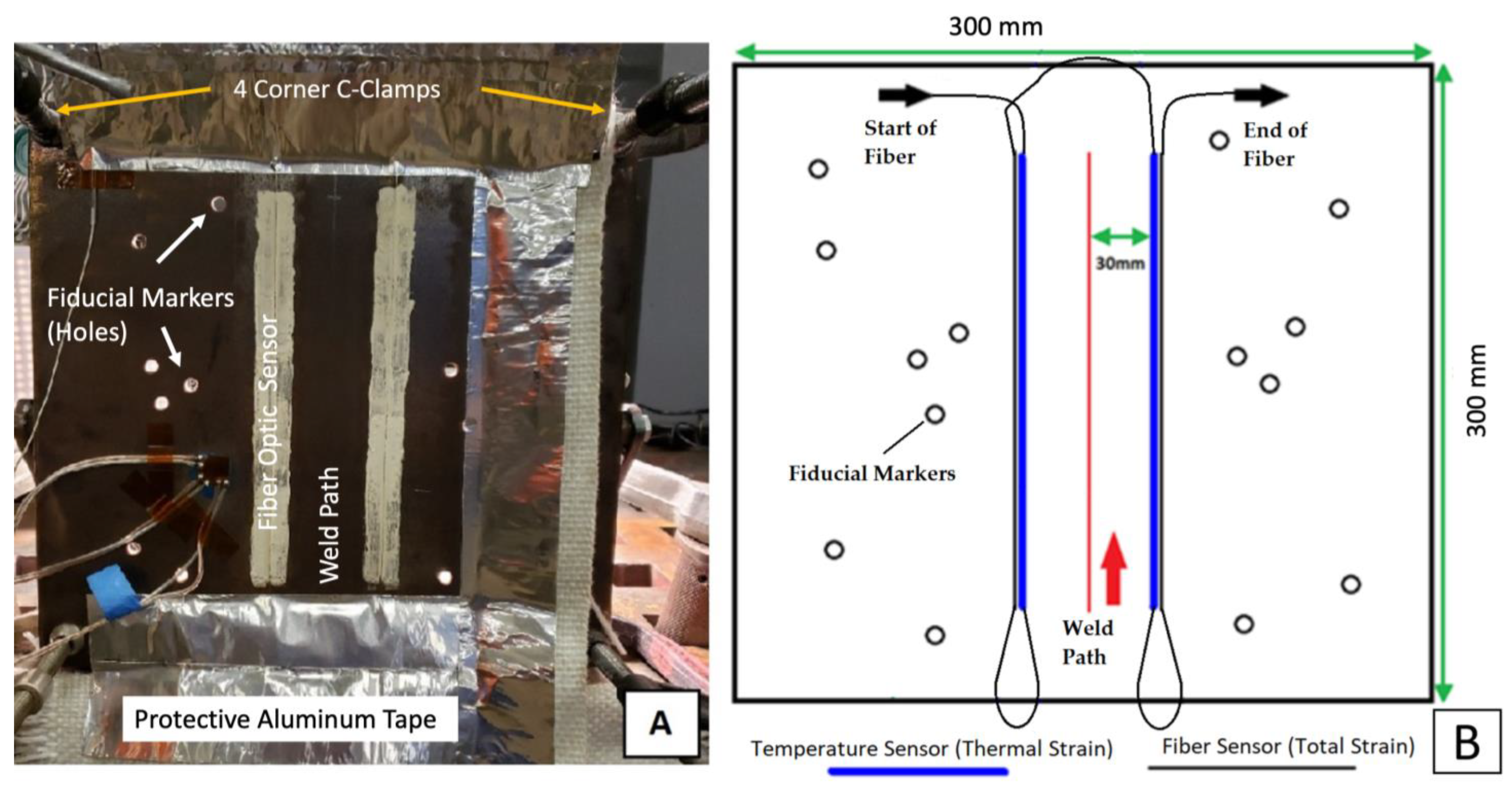
2.2. Specimen Instrumentation

The polyamide-coated fiber optic sensor was attached to the front surface of the specimen parallel to the weld path. Prior to attaching the fiber optic, the surface was sanded to remove surface oxidation. Resbond 904 epoxy was used to adhere to the fiber optic because of its high-temperature qualities [22]. Resbond 904 is rated up to 2204 °C [22]. One fiber segment adhered to the surface of the plate while a second parallel segment of the fiber was inserted inside a PTFE tube to allow for free movement of the fiber and thus measure the thermal strains as indicated by the thicker lines in Figure 1B. It was important to ensure that the ends of the fiber exiting the PTFE tube were free to move once the Resbond 904 adhesive paste was applied. Once the fiber optic was set in place, Resbond 904 was applied and allowed to cure for 24 h at room temperature. After 24 h, the ultra-high temperatures Zirconia adhesive (Resbond 904) was fully hardened, thus covering both the PTFE tube/sensor (temperature sensor) and fiber optic sensor (total strain sensor). The adhesive serves as a protective coating and holds both the fiber and PTFE tube in direct contact with the steel plate. Other adhesives had been used (M-Bond 200, only rated to 200 °C), and it was observed that M-Bond 200 would not withstand the high temperature in the proximity of the weld path. The authors observed that the fiber and the PTFE tube would disbond from the steel plate once the weld was completed with M-Bond 200. In the case of Resbond 904, both the fiber and the PTFE tube remained bonded to the steel plate after completion of the weld.

2.3. Experimental Method

In this study, a LUNA ODISI-B system based on Rayleigh backscattering principle for measuring strain was used. The primary advantage of this type of system is its ability to provide extremely high spatial resolution. In the case of the LUNA ODISI-B system, a spatial resolution of 0.65 mm up to a 10 m-long fiber at a data acquisition rate of 23.8 Hz is reported by the original equipment manufacturer [23].

In addition to the use of the fiber optic, the authors positioned a FLIR One Pro thermographic camera facing the back of the plate [24]. Previous studies [7] have shown good correlation between the use of commercial off-the-shelf inexpensive cameras and VrWeld predicted results. This also presented an opportunity for comparing 3 independent techniques: (i) FODSS; (ii) FLIR One Pro thermographic camera connected to an iPhone XI [25]; and (iii) VrWeld. It is important to add that this was a commercial off-the-shelf non-scientific camera which is only capable of measuring temperatures accurately below 400 °C. In addition, to preserve the thermographic data, an operator must take photographic data manually. In other words, the use of thermographic video prevents the authors from analyzing the individual frames of the video at a later stage. As the thermographic images are taken manually, this creates an additional challenge in the synchronization of the thermographic data. This was dealt with by understanding the position of the weld pool in time with respect to the fiducial markers shown in Figure 1. The use of a common stopwatch which was captured by the thermographic camera and the DIC cameras allowed us to sync all the data at any moment in time during the welding of the bead on plate.

3. Computational FEA with VrWeld

To achieve the objectives of this study, the experimental team at Clarkson University worked independently from the CWM team at Goldak Technologies Inc. (Ottawa, ON, Canada) It is important to note, that the two teams had been collaborating in this type of research for over the past 5 years, with varied levels of success. In part, the challenge of synchronizing experimental and computational data is not a straightforward task. As such, many of the previous attempts to compare CWM and experimental data failed due to the inability to synchronize computational and experimental results in both space and time. This section of the study aims to outline the basic aspects of the FEA. A general overview of the workflow for a VrWeld analysis in a structure is depicted in Figure 2. Each rectangular box with rounded corners is a solver, usually a 3D transient non-linear FEM solver. The diamond shapes represent the inputs to the solver, while the elliptical shapes represent the outputs. VrWeld is a physics-based model. As such, the internal algorithm computes the transient temperature, the microstructural evolution, and the transient evolution of the displacement, strain, and stress tensor fields while welding a structure. VrWeld has been validated in previous studies; however, this validation took place through the use of classical sensors such as strain gauges and thermocouples at discrete points [26,27]. In this paper, an attempt was made to validate VrWeld by measuring the correlation between measured and predicted temperatures and strain fields utilizing a fiber optic distributed sensing system at multiple points along the fiber.

The inputs required for this analysis consist of (i) the geometry of all parts, alloy types that define the composition and initial synthetic microstructure, and (ii) the weld procedure that defines the parameters of the welding process. The solvers represented by rectangular boxes in Figure 2 consist of the following:

1.

The FEM/SPH WP solver computes a macroscopic transient temperature and the WP geometry by solving the Conservation of Energy equation as outlined in Equation (1):

$$\dot{h}+\nabla ·q+Q=0$$

(1)

where $\dot{h}$ is the rate of change of the specific enthalpy, q is the thermal flux, and Q is the power density function. The thermal flux can be expressed as

$$q=-\mathsf{\kappa }·\nabla T$$

(2)

where κ is the thermal conductivity tensor, and ∇T is the temperature gradient at a point. In addition, the change in specific enthalpy is expressed as

$$dh=c_{p}dT$$

(3)

where $c_p$ is the specific heat and dT represents the temperature change. VrWeld solves this partial differential equation on a domain defined by a FE mesh. In this study, the steel plate was modeled using a mesh of 147,360 eight-node brick elements. The element size was generally 2 mm × 2 mm × 2 mm around the plate; however, near the weld, this was reduced to 1 mm × 1 mm × 0.8 mm. This translates into six eight-node bricks across the width, and ten along the length, of the weld pool, which has been found to resolve the transient temperature field around the weld pool adequately. This satisfies the requirements established by ISO Document ISO/TC 44/WG 5—Welding simulation [28]. The initial condition is assumed to be a constant temperature of 300 °K. The material properties κ and $c_p$ are temperature and microstructure dependent. The heating effect of the arc is often modeled by a double ellipsoid power density distribution that approximates the WP as measured from macro-graphs of the cross-section of several weld passes [29]. A convection boundary condition q = h (T − T_amb) is applied to external surfaces. The FEM formulation of the heat equation leads to a system of ordinary differential equations that are integrated in time using a backward Euler integration scheme. Finally, this solver computes the thermal cycle as an output which serves as an input into the Austenite–Ferrite microstructure solver. The solvers were written in C++ over the last 20 years by Goldak Technologies Inc. for the analysis of welds. They are based on numerical algorithms described in [30] and the references therein.

Figure 2. The workflow for a VrWeld analysis of a weld in a structure. Each rectangular box with rounded corners is a solver, usually a 3D transient non-linear FEM solver. (1) Represents the FEM Weld Pool Solver; (2) Represents the Austenite Ferrite Solver; (3) The Carbon Diffusion Solver; (4) the Microstructure Solver, while (5 and 6) are the stress solvers in charge of determining residual stress and strains and micros stress-strain curves [31].

Figure 2. The workflow for a VrWeld analysis of a weld in a structure. Each rectangular box with rounded corners is a solver, usually a 3D transient non-linear FEM solver. (1) Represents the FEM Weld Pool Solver; (2) Represents the Austenite Ferrite Solver; (3) The Carbon Diffusion Solver; (4) the Microstructure Solver, while (5 and 6) are the stress solvers in charge of determining residual stress and strains and micros stress-strain curves [31].

2.

The austenite–ferrite solver computes the transient decomposition of ferrite to austenite and then to liquid upon heating. This analysis is followed by the transient transformations of the liquid to austenite, ferrite, pearlite, bainite, and martensite upon cooling, depending on the composition of the steel base metal. The output of this solver is the carbon composition and new grain microstructures serving as the input to the carbon-diffusion solver.

3.

The carbon-diffusion solver computes the diffusion of carbon between phases in each transient phase transformation of heating and cooling.

4.

The microstructure solver computes the nucleation and growth of phases based on equilibrium thermodynamics, i.e., the phase diagram for the composition, temperature, and pressure of the system, and irreversible thermodynamics, i.e., the second law of thermodynamics—kinetics, entropy, and dissipation. However, there is not enough space to deal with these complex phenomena in this manuscript.

5.

The stress solver computes transient stress during the welding process. When the structure has been welded, cooled down and any constraints have been removed, the stress that remains is called the RS.

6.

The stress solver takes the initial state with RS, microstructure, and distortion from the as-welded structure and applies in-service loads applied to the welded structure.

The stress solver is based on the conservation of momentum equation. Given the fields for density, ρ, the elasticity tensor as a 6 × 6 matrix, the body force b, the Green-Lagrange strain ε, temperature, coefficients of thermal expansion, and phase fractions for each microstructure field as a function of time and space, VrWeld solves the conservation of momentum equation that can be written in the following form in which inertial forces ($\rho \ddot{x}$) are ignored:

$$\nabla ·\sigma +b=0$$

(4)

The stress tensor ($\sigma )$ is defined as

$$\sigma =D\epsilon$$

(5)

where D represents the elasticity tensor as a 6 × 6 matrix and $\epsilon$ represents the strain.

The initial state was assumed to be stress-free. The Dirichlet boundary conditions (BCs) constrain the rigid body modes. The system is solved using a time marching scheme to compute increments in displacement, strain, and stress. The time step lengths are approximately 1 s during welding and usually, an exponentially increasing time step length begins when the welding stops and is applied until the structure cools to ambient temperatures. The arrows shown in Figure 2 are indicative of the data flow, with state variables mapping from one solver to the next.

Table 1. Material Properties for A36 Plate.

Material	Tensile Strength lb/in2, [MPa]	Yield Strength lb/in2, [MPa]	Elongation in 2 in. (%)	Reduction of Area (%)
A36 Steel Plate	63,800	53,700	15	40
	[439.9]	[370.20]

indicates the material properties used in VrWeld to model the bead-on-plate, while the assigned thermal conductivities of the plate were taken from [7]. The results of the VrWeld model were essential for determining the thermal and total strain behavior during and post-weld for validation of the experimental results.

The stress analysis for this study run on a 2010 four-core Intel CPU with an NVIDIA 750 GPU card for approximately 2 h. The model does not apply Dirichlet BCs to approximate the action of the corner clamps shown in Figure 1A. This is because the measured strain at the fiber sensor location on the plate was small (less than 200 microstrains). The VrWeld model filtered the rigid body motion as documented in [32]. However, for the thermal and microstructural analysis, the CPU time was about 15 min.

4. Experimental Results

In many welding studies found in the open literature, the computational model is validated through experimental data sets. However, in this study, it was the reverse; it was the computational models that helped identify challenges in fiber optic measurements. This section of the study is divided into three sections: (i) power curve during the manual welding of the bead on plate; (ii) fiber optic strain results; and (iii) VrWeld computational results.

4.1. Welding Power

A camera facing the welder power supply and connected to the DIC DAQ system took snapshots of the voltage and current digital readouts at one-second intervals. The team translated data from the images into an Excel spreadsheet from which power could be calculated at every instant during the welding process. This test consisted of a continuous bead-on-plate weld with an average power of approximately 2500 W. The welding process lasted approximately 100 s.

4.2. Fiber Optic Strain Results

Figure 3 shows a closeup of the total strain measured by the fiber optic along the entire fiber optic line. As shown in Figure 3, Segments 1 and 4 correspond to the fiber sections measuring the thermal strain. The primary difference between temperature sensing and total strain sensing is the embedding of fiber segments in a PTFE tube. Thus, the thermal strain allows the fiber optic line to slide freely into the PTFE tube. These thermal segments correspond to fiber lengths from 0.475 to 0.679 and 1.85 to 2.054 m, respectively. As such, the thermal strain in this region of the fiber starts at zero, reaches a maximum strain between 3000 and 3500 µε (microstrains), and drops back down to zero once the temperature in that section of the fiber reaches room temperature. Segments 2 and 3 of the fiber correspond to sections of the fiber that measure total longitudinal strain, as they are adhesively bonded to the A36 steel plates.

As seen in Figure 3, the thermal sections of the fiber over-predicted the thermal strain. This is primarily because of the over-constraint produced by the PTFE on the fiber, thus impeding the fiber from sliding within the tube as the plate is heated due to the passing of the weld pool. The PTFE tube has a 1 mm outer diameter and 0.6 mm inner diameter. The fiber optic is 150 microns in diameter, as indicated in Figure 3. This figure shows the fiber positioned on top of the steel plate without the adhesive. As seen in the figure, a second section of the fiber (Total Strain Fiber in Figure 3) is placed beside the PTFE tube to measure the strain on the steel plate during the welding process.

Since the fiber is a continuous fiber, during welding there are sections of the fiber that are in line with the welding direction, while other sections of the fiber are against the welding direction, as shown in Figure 1. That is why Sections 1 and 2 are symmetrical to Sections 3 and 4. Based on the original placement of the fiber, Section 1 was set to be against the welding direction, while Section 2 was in the same direction as the weld. Section 3 was set to be against the welding direction, while Section 4 was in line with the welding direction. This is important during the post-processing of the data because when compared to the Finite Element Model, the data needs to be re-aligned towards the welding direction.

The fiber optic sensors for the bead-on-plate included two total longitudinal and two thermal strain sections at 30 mm on either side of the weld path, as shown in Figure 1B. The results captured by the FOS consisted of transient longitudinal strains. During the experiment, the peak tensile longitudinal strain during the weld was noted to be 3414 µε and the residual compressive strain after cooling reached −1008 µε as seen in Figure 4. Figure 4A shows the longitudinal total strain on the side of the plate that has the fan predominantly blowing on its backside, while Figure 4B shows the section of fiber on the adjacent side. The effect of the fan resulted in a difference in peak strains of approximately 100 µε at 88 s. Although this does not seem significant, this translates into a difference of approximately 500 µε in residual strains on the plate after 0.8 h of cooling, as shown in Figure 4A,B. Figure 4C,D show the thermal strain which can then be converted to surface temperature by knowing the thermal expansion coefficient of the fiber. As seen in these figures, they reach values of approximately 3300 and 3400 µε, respectively. However, thermal strain drops back to 250 µε after 0.8 h of cooling. Thermal strain can be transformed into a change in temperature measurement by dividing the thermal strain measured by the thermal expansion coefficient of the fiber, 8.5 µε/°C, and adding the initial room temperature at time zero, as shown in Figure 4C,D. As can be observed in these figures, the temperature along the weld path at 30 mm from the weld line is approximately 430 °C at 88 s. However, after approximately 3000 s, this temperature tends to drop back to room temperature, and thus the thermal residual strain drops back to zero in these fiber sections. However, for reasons explained in the discussion section of this manuscript, it was determined that the thermal strains are overestimated due to over-constraints of the PTFE tubing on the fiber optic section past approximately 250 °C. The authors of this study considered it important to showcase and document the erroneous thermal measurement, so as to inform the welding community and avoid repeats in the future. It is important to note that the LUNA DSS is actually accurate in the measurement technique. However, PTFE at high-temperature applications is not recommended. It is commonly considered that CWM is validated through experimental measurements, the gold standard. However, this is a case that generated over 2 years of discussion between the experimental team at Clarkson University and Goldak Technologies Inc. in attempting to synchronize and validate the findings.

The fiberoptic data can also be plotted in time versus fiber length with respect to strain as shown in Figure 5. This type of graph shows the entire fiber optic sensor stain measurement over time. The figure has been divided into multiple Sections 1–4. Sections 1 and 4 represent the sections of the fiber that are embedded in a Teflon tube, thus acting as temperature sensors, while Sections 2 and 3 represent the sections of the fiber that are attached to the steel plate. At approximately 1.3 m, the figure shows the weld path. The color gradient range was set from 2000 (tensile) to −2000 µε (compression) to depict the dynamic formation of residual strains during the cooling process.

As seen in Figure 5, the thermal sections of the fiber are highly tensile from zero to 200 s and cool down to zero µε (back to room temperature) over time. Sections 2 and 3 of the fiber capture total strain and show a clear tensile behavior of that section of the plate. However, as it cools down, those same sections become compressive in nature, indicative of the residual strains formed during the cooling process. It is interesting to note that Section 2 cools down to just −500 µε while Section 3 is closer to −1000 µε. The effects of the fan cooling in Section 2 shows how the residual strain formation can be minimized by proper cooling during the welding process. The fan was strategically placed at an angle to avoid the heat formation between the back of the plate and the DIC cameras.

5. VrWeld Results

The initial objective of this work was to use the experimental results to validate the VrWeld model. The primary assumption was that the experiments would provide the correct results which the VrWeld model needed to match. Figure 6 shows the transient thermal strain results from the FODSS and VrWeld. As it is observed in this figure, the initial thermal strains are over-predicted by VrWeld (at 16 s, LUNA clock), while they match very nicely after 28 s (LUNA clock). It is hypothesized that the thermal sensor time lag is due to the thermal conductivity of the PTFE tube, requiring time for heat transfer into the core of the fiber. Another important observation is that the thermal strain gradients in front of the WP match closely. This is indicative of the ability of the FOS to measure and spatially resolve the thermal strain gradient and thus the transient temperature field when the weld is in the proximity of a steady state condition.

Figure 7 shows the temperature profile along Section 1 at 88 s. A comparison between the VrWeld predicted temperature and the fiber optic sensing data shows large temperature differences (approx. 200 °C) at this time step. The experimental team at Clarkson University and the CWM team at Goldak Technologies Inc. had many discussions on what was causing these differences. After many simulations and iterations (over 2 years), the authors came across an article by Prof. Xiaoyi Bao [33]. This led to direct communication with Prof. Bao on the use of distributed FOS for temperature measurements. Prof. Bao recalled a non-published experiment in which she encased a fiber optic in a PTFE tube which was subsequently encased in a heated quartz tube. The result of that experiment showed how the PTFE tube expanded and broke the quartz tube. Based on this experience, it was hypothesized that because PTFE has a high coefficient of thermal expansion, it could expand at high temperatures over constraining the polyamide fiber, leading to an overestimation of the temperature measurement. In our study, the PTFE tube was encased in the ceramic Resbond 904 adhesive, as such it was hypothesized that hydrostatic strain formed due to the PTFE tube expanding at high temperatures. Prof. Xiaoyi Bao’s conjecture is consistent with the temperature measurement along the fiber optic sensor. At lower temperatures (Figure 7) the measured and predicted temperatures agree while at higher temperatures when the PTFE expands, the measured temperatures are as much as 1.9 times higher than the temperatures predicted by VrWeld.

To validate Prof. Bao’s statement, the authors of this study made an additional comparison utilizing the FLIR One Pro camera located at the back of the plate with the temperature field computed by VrWeld. A quick evaluation of the VrWeld model indicated that the temperatures at the front and back of the plate were almost identical, as the plate was only 6.5 mm thick. Figure 8a shows the thermographic data processed through the FLIR SDK MATLAB^TM script [34]. The dashed white line in the figure is indicative of the position of the fiber optic sensor. Figure 8b clearly shows how both the FLIR temperature field at the back and VrWeld data at the front of the plate match very nicely at 76 s. This result is indicative that the thermographic data and VrWeld result are synchronized and produce very accurate results from a temperature gradient and dynamic perspective.

In order to validate the performance and accuracy of the fiber optic sensor, a steel plate with a thermocouple and a fiber optic sensor embedded in a PTFE tube was inserted into an oven and heated to approximately 500 °C. Figure 9 shows the fiber optic thermal strain with its corresponding secondary y-axis showing the equivalent temperature measured by the FODSS. The star symbols at the 1.45 m position represent the temperatures measured by a K-type thermocouple. This figure shows how at zero seconds, the thermocouple measures room temperatures (23 °C) coinciding with a fiber optic temperature measurement. This process was repeated at 1500 s and 2000 s. At both times, the thermocouple and fiber optic measurements matched. However, at approximately 3000 s from the initiation of the experiment, the thermocouple read approximately 444 °C, while the fiber optic sensor predicts the measurement by approximately 350 °C. This is indicative of Prof. Bao’s statement that at higher temperatures above 250 °C, the fiber optic distributed sensor is unable to capture the correct temperature measurement. It is important to note that this over-prediction is not from the inability of the LUNA distributed sensing system but rather the use of a Teflon tube as a protective sleeve whose primary objective is to allow the free movement of the internal fiber due to temperature changes. The PTFE tube constrains the fiber optic sensor. Thus, the actual measurement at any temperature above 250–300 °C is a combined thermal and mechanical strain measurement.

Direct comparisons of the VrWeld total strain measurement and the FOS at the front of the plate are found in Figure 10. This figure represents the longitudinal strain (along the fiber length) at the x-position of 123 mm and y-positions of 140, 160, and 180 mm, as outlined in Figure 8a. A total of three positions along the CWM model and the fiber optic sensor were chosen so as to determine if the overall total strain behavior of the fiber was consistent with the behavior visually captured by VrWeld. In this part of the study, the authors were interested in capturing the steady-state behavior of a manual weld. Figure 10 shows how the LUNA fiber optic total strain reaches close to 1850 µε while VrWeld shows a maximum peak strain close to 1500 µε. The CWM team believes that a 350 µε difference at the peaks is not unreasonable considering the complexity of a manual weldment and the amount of data being analyzed and synchronized for validation. It is also important to note that 200 to 250 µε are equivalent to the clamping of the plate at the corners prior to the start of the weld. It is observable that the total strain gradients between VrWeld and the FOS match very nicely. The shift in the strain as the WP moves up along the plate is also captured, and the strain gradient at the back of the WP also matches closely between VrWeld and the FOS system. An important observation shows that a small compressive residual strain is computed by VrWeld which is not seen by the fiber optic system, which is because the FOS is zeroed out (tared) prior to the commencement of the welding process. This taring of the system is performed as the FOS measures changes in strain due to mechanical and/or thermal loads. It does not measure absolute strain values. In the case of the total strain section of the fiber, this needs to be zeroed due to the hardening of the adhesive, which generates a series of residual strains on the fiber itself. However, in the case of temperature measurement, a thermocouple is used to relate the initial room temperature to zero strain measured by the FOS. The thermal expansion of the fiber is a constant and thus allows us to compute the equivalent temperature for a change in strain. That is how in Figure 9, zero strain on the first y-axis is equivalent to 23 °C on the secondary y-axis, while approximately 2500 µε is equivalent to 300 °C.

However, despite these achievements, the authors of this study wanted to understand the performance of the FOS during the transient total strain measurements at the beginning and end of the weld, when the arc was being turned on and off, respectively. Figure 11 shows the transient total strain at the start and end of the weld. The results of the FOS were compared to the VrWeld total strain at the same location and time. As observed, the total strain measurement response lags in comparison to the VrWeld results during both the heating and cooling stages when the arc is being turned on and off. At the start of the weld, at a position 60 mm from the bottom of the plate, there was approximately an additional 12 s shift, even though the peaks of total strain are in line and the strain gradients match with those computed by VrWeld. However, at the end of the weld (100 s), the total strain peaks are off by approximately 500 µε. The cooling of the FOS is noticeably consistent at the start and end of the weld, while VrWeld cooling gradients are much steeper. This is in contrast with Figure 10, where both the peaks and the total strain gradients at the front and back of the weld pool are in sync during the steady state condition of the weld. The authors hypothesize that the transient heating and cooling in front and at the back of the weld pool requires further analysis and evaluation by both the CWM and experimental mechanics teams. It is possible that the lack of synchronization during the transient analysis could be a combination of factors on how the strain is transferred to the core of the fiber through the Resbond 904 and the steel plate. The CWM team also agrees that further investigation with millisecond discretization range and high-speed DIC would be required to truly understand the physics during the arc turning on and off.

6. Discussion

Distributed FOS is emerging as an alternative to conventional strain measurement techniques. Conventional techniques such as strain gauges are not as efficient in providing an array of temperature and strain measurements along a weld path. The ability to measure strain within ±12,000 µε in addition to being functional in a high-temperature environment can become a useful tool for unraveling the complex physics of strain formation in welding applications. However, this study demonstrated that although Rayleigh backscattering can accurately measure total strain, the encapsulating material used for temperature measurements needs to be rethought. Future studies will require the authors to investigate another material tube to avoid the inner fiber from being affected by the thermal expansion of the encapsulating tube. As such, the use of PTFE tubing as a FOS temperature sensor was shown to be ineffective in this type of harsh high-temperature environment.

The results presented in this study showcase the inability of the fiber optic sensor to measure temperatures above 250–300 °C in this experiment. In addition, it also demonstrated the need for sensing fibers that can measure closer to the WP. In previous studies, not reported in this manuscript, fibers closer than 30 mm were unable to withstand the high-temperature fields and caused the fibers to burn during the arc welding. Furthermore, it was shown that Resbond 904 adhesive held up very well at high temperatures. It is important to note that other adhesives had been previously attempted, such as M-Bond 200, which showed incorrect behavior for both the thermal and total strain past 200 °C. It is important to note that it was the combination of experimental mechanics and computational models that allowed the authors to recognize that this behavior was not consistent with the physics of the weld being analyzed.

The total strain measurement sections of the fiber are in direct contact with the steel plate, as such it measures the total strain in the direction of the fiber, in this study the longitudinal strain. Polyimide-coated fibers are preferred due to their high-strength fibers versus acrylate-coated fibers. The use of polyimide coating allows for a good transfer of strain from the base material of interest to the fiber core. These sections of fiber measure a zero-strain value as a baseline reading, recorded once the fiber is adhesively bonded to the structure (at room temperature) and the plate is fully clamped. The system allowed us to measure the longitudinal strain due to clamping. It was observed that the average strain at 30 mm away from the weld path due to clamping is approximately 200 to 250 µε.

It is important to note that FOS used (LUNA ODISI-B) does not distinguish thermal and mechanical strains from each other. As such, when applying the FOS technique in the welding process which experiences large temperature gradients, it was necessary to isolate these components from each other. Newer techniques are being sought out to decouple the thermal and mechanical strains at the same point on the same section of fiber. The approach utilized in this study creates uncertainties when extracting the mechanical strain component, and hence it was not presented in this manuscript.

Despite the many advancements in the use of DSS, the use of this system to compute mechanical strain (difference between total and thermal strain) is not a trivial task. Attempts to perform this type of analysis at the same exact point in the fiber would require being able to pinpoint the exact position in the total and thermal fiber section. Although it could be accomplished by pressing both thermal and total fiber segments with a ruler at the same location, as the thermal fiber is free to move during handling, it is possible for the thermal section of the fiber to slide in and out of the PTFE tube during the experimental setup. Attempts by the authors showed that slight differences in the position of the thermal strain point of interest can substantially change the mechanical strain computed. If the position of the thermal strain and the total strain are not at the same location as the plate, it translates into large differences in mechanical strain measurements. Attempt to evaluate mechanical strains at the peaks of the total and thermal strain also resulted in incorrect outcomes. As the fiber optic is freely allowed to move while it is being heated, a shift in position from an initial location can result in large variations. The fiber optic can capture a strain measurement every 0.65 mm. Initial attempts to subtract the thermal strain from the total strain resulted in large variations in the results depending on which point within the fiber was taken.

7. Conclusions

The formation of transient strain and temperature fields of a manual weld has been examined with the primary goal of understanding the intricacies required to compare CWM models with big data obtained from experimental mechanics techniques. The use of distributed sensing fiber optic systems has been shown to be accurate and an efficient means of obtaining hundreds of total strain data points in the proximity of the weld line and within the limitation of the fiber sensor. However, it has also been shown that the materials used for the development of thermal fiber optic strain sensors must be carefully thought-out for high-temperature applications. This study highlights the need for the experimental and CWM teams to discuss critical items a priori of any verification tests, such as (i) knowledge of the welding power; (ii) the use of fiducial markers within the structures being welded; (iii) synchronization of multiple independent DAQ systems through a single clock; (iv) development of software that can handle the big data sets being captured; and finally (v) a clear communication line between the experimental and the CWM groups attempting to synchronize results obtained for complex physical welding processes.

It is important to highlight that it is usually the experimental techniques that validate the CWM models. However, in this study, the reverse occurs, it was the CWM team that was able to demonstrate how the thermal sensor was overestimating the temperature fields. Thus, averting the experimental team from publishing data that from all perspectives looked reasonable but turned out to be erroneous. It is important to note that the LUNA DSS is accurate in measuring strain, but that the fabrication of thermal sensors must be carefully considered for high-temperature applications, including the time lag that the thermal barrier may have on the temperature measurement. The use of a DSS fiber optic system allows for large data sets on strain and temperatures (below 250 °C) for evaluation of CWM FEM, versus discrete foil strain gauges and/or thermocouples. Thermography and DIC have been used by the authors and other researchers successfully. However, special filtering techniques and care for capturing the full field of view at the front of the plate using DIC and/or thermography are required. It is also important to highlight the need to repeat this type of experiment with automated arc welding systems and consider an experimental setup focused on transient welding, i.e., spot welding conditions to better understand the transient nature of the weld.

Finally, transient analysis during welding is a complex endeavor. The welding community has successfully understood the steady state behavior and the formation of residual strain/stresses at the end of the welding process. However, many of these studies lack an understanding of the challenges of synchronization of both temporal and spatial data sets. In addition, it has been the intention and belief of the authors in this study that to understand the intricacies of welding, it is essential to understand the transient aspects of the process. Furthermore, the experimental mechanics team learned a valuable and humbling lesson that experiments are very sensitive to many variables. The major lesson learned was that the combination of both computational and experimental models needs to be carefully analyzed and compared to ensure that the scientific method is followed. The CWM team was able to validate their models and work with an independent experimental team and adapt their models for comparison with larger distributed data sets, not just a couple of strain gauges and thermocouples. This study aimed to open the door for further research on the need to evaluate the transient behavior of welding processes and the challenges outlined in the verification and validation of this complex manufacturing technique.

References

1. Maddox, S.J. Fatigue design rules for welded structures. Prog. Struct. Eng. Mater. 2000, 2, 102–109. [Google Scholar] [CrossRef]
2. Taniguchi, K.; Lim, Y.C.; Flores-Betancourt, A.; Feng, Z. Transient Microstructure Evolutions and Local Properties of Dual-Phase 980 MPa Grade Steel Via Friction Stir Spot Processing. Materials 2020, 13, 4406. [Google Scholar] [CrossRef] [PubMed]
3. Sutton, M.A.; Orteu, J.-J.; Schreier, H. Image Correlation for Shape, Motion and Deformation Measurements: Basic Concepts, Theory and Applications; Springer Publishing Company, Incorporated: Berlin/Heidelberg, Germany, 2009. [Google Scholar]
4. Yin, S.; Ruffin, P.B.; Yu, F.T.S. Fiber Optic Sensors, 2nd ed.; CRC Press—Taylor & Francis Group: Boca Raton, FL, USA; London, UK; New York, NY, USA, 2008. [Google Scholar]
5. Freddi, A.; Olmi, G.; Cristofolini, L. Experimental Stress Analysis for Materials and Structures: Stress Analysis Models for Developing Design Methodologies. In Springer Series in Solid and Structural Mechanics Book, 4th ed.; Frémond, M., Maceri, F., Eds.; Springer: Cham, Switzerland; Heidelberg, Germany; New York, NY, USA; Dordrecht, The Netherlands; London, UK, 2015. [Google Scholar]
6. De Strycker, M.; Lava, P.; Van Paepegem, W.; Schueremans, L.; Debruyne, D. Measuring welding deformations with the digital image correlation technique. Weld. J. 2011, 90, 107S–112S. [Google Scholar]
7. Pliazhuk, M.; Reyes, C.; Martinez, M.; Goldak, J.; Nimrouzi, H.; Aidun, D.K. In-situ Monitoring of Transient Strain Formation in Vertical Welds. Weld. J. (AWS) 2019, 98, 251–262. [Google Scholar]
8. Chen, J.; Yu, X.; Miller, R.G.; Feng, Z. In situ strain and temperature measurement and modelling during arc welding. Sci. Technol. Weld. Join. 2015, 20, 181–188. [Google Scholar] [CrossRef]
9. Hagenlocher, C.; Stritt, P.; Friebe, H.; Blumenthal, C.; Weber, R.; Graf, T. Space and time resolved determination of thermomechanical deformation adjacent to the solidification zone during hot crack formation in laser welding. In Proceedings of the International Congress on Applications of Lasers & Electro-Optics, Orlando, FL, USA, 14–18 October 2018. [Google Scholar]
10. Keller, D., Jr. Comparison of Resistance-Based Strain Gauges and Fiber Bragg Gratings in the Presence of Electromagnetic Interference Emitted from an Electric Motor; Department of Mechanical Engineering, University of Alaska Fairbanks: Fairbanks, AK, USA, 2018. [Google Scholar]
11. Barazanchy, D.; Martinez, M.; Rocha, B.; Yanishevsky, M. A Hybrid Structural Health Monitoring System for the Detection and Localization of Damage in Composite Structures. J. Sens. 2014, 2014, 109403. [Google Scholar] [CrossRef]
12. Luis Rodriguez-Cobo, J.M.; Ruiz-Lombera, R.; Cobo, A.; López-Higuera, J.-M. Fiber Bragg grating sensors for on-line welding diagnostics. J. Mater. Process. Technol. 2014, 214, 839–843. [Google Scholar] [CrossRef]
13. Suárez, J.C.; Remartınez, B.; Menéndez, J.M.; Güemes, A.; Molleda, F. Optical fibre sensors for monitoring of welding residual stresses. J. Mater. Process. Technol. 2003, 143, 316–320. [Google Scholar] [CrossRef]
14. Petrie, C.M.; Sridharan, N. In situ measurement of phase transformations and residual stress evolution during welding using spatially distributed fiber-optic strain sensors. Meas. Sci. Technol. 2020, 31, 125602. [Google Scholar] [CrossRef]
15. Schricker, K.; Ganß, M.; Könke, C.; Bergmann, J.P. Feasibility study of using integrated fiber optical sensors to monitor laser-assisted metal–polymer joining. Weld. World 2020, 64, 156–1578. [Google Scholar] [CrossRef]
16. Van De Giesen, N.; Steele-Dunne, S.C.; Jansen, J.; Hoes, O.; Hausner, M.B.; Tyler, S.; Selker, J. Double-Ended Calibration of Fiber-Optic Raman Spectra Distributed Temperature Sensing Data. Sensors 2012, 12, 5471–5485. [Google Scholar] [CrossRef]
17. Mizuno, Y.; Hayashi, N.; Tanaka, H.; Wada, Y.; Nakamura, K. Brillouin scattering in multi-core optical fibers for sensing applications. Sci. Rep. 2015, 5, 11388. [Google Scholar] [CrossRef] [PubMed]
18. Rahim, N.A.A.; Pandher, J.; Coppola, N.; Penumetsa, V.; Michel, D.; Tooren, V. In-situ monitoring and control of induction welding in thermoplastic composites using high definition fiber optic sensors. In Proceedings of the Composites and Advanced Materials Expo, CAMX, Anaheim, CA, USA, 17–20 October 2022. [Google Scholar]
19. Martinez-Bueno, P.; Martinez, M.; Rans, C.; Benedictus, R. Strain Monitoring using a Rayleigh Backscattering System for a composite UAV wing instrumeted with an embedded Optical Fiber. Adv. Mater. Res. 2016, 1135, 1–19. [Google Scholar] [CrossRef]
20. Baldassarre, A.; Ocampo, J.; Martinez, M.; Rans, C. Accuracy of Strain Measurement Systems on a Non-Isotropic Material and its Uncertainty on Finite Element Analysis. J. Strain Anal. Eng. Des. 2020, 56, 76–95. [Google Scholar] [CrossRef]
21. Edmund, E. FLIR Grasshopper High Performance USB 3.0 Cameras. 2022; High Performance USB 3.0 Cameras for Digital Image Correlation. Available online: https://www.edmundoptics.com/f/flir-grasshopper3-high-performance-usb-30-cameras/14785/ (accessed on 20 March 2022).
22. Cotronics Corporation, 4000°F Resbond™ 904 Ultra Temp. 2022. Available online: http://www.cotronics.com/vo/cotr/ca_onecomp.htm (accessed on 20 March 2022).
23. Luna Innovations Inc., Optical Distributed Sensor Interrogator. 2021. Available online: https://lunainc.com/sites/default/files/assets/files/data-sheet/ODB5_DataSheet_Rev13_020217.pdf (accessed on 20 March 2022).
24. Teledyne FLIR, FLIR One Pro. 2022. Available online: https://www.flir.com/products/flir-one-pro/ (accessed on 20 March 2022).
25. Apple Inc., iPhone X. 2017. Available online: https://www.apple.com/newsroom/2017/09/the-future-is-here-iphone-x/ (accessed on 12 September 2017).
26. Bayley, C.; Goldak, J. Welding Induced Distortions and Strains of a Built-Up Panel, Experiment and Numerical Validation. J. Press. Vessel Technol. 2012, 134, 021212. [Google Scholar] [CrossRef]
27. Goldak, J.; Asadi, M. Challenges in Verification of CWM Software to Compute Residual Stress and Distortion in Weld. In Proceedings of the International ASME 2010 Pressure Vessel and Piping Division Conference, Bellevue, WA, USA, 18–22 July 2010. [Google Scholar]
28. Standard, I. Welding and Allied Processes. 1947; Standardization of Welding, by All Processes, as well as Allied Processes; These Standards Include Terminology, Definitions and the Symbolic Representation of Welds on Drawings, Ap-Paratus and Equipment for Welding, Raw Materials (Gas, Parent and Filler Metals) Welding Processes and Rules, Methods of Test and Control, Calculations and Design of Welded Assemblies, Welders’ Qualifications, as well as Safety and Health. Available online: https://www.iso.org/committee/48602.html (accessed on 22 March 2023).
29. John Goldak, E.J.; El-Zein, M.; Zhou, J.; Tchernov, S.; Downey, D.; Wang, S.; Coulombe, M. The L2 norm of the deviation between the measured and computed transient displacement field in a test weld. In. J. Mat. 2008, 99, 428–433. [Google Scholar]
30. Simo, J.C. Numerical Analysis of Classical Plasticity, Handbook for Numerical Analysis. Handb. Numer. Anal. 1988, VI, 183–499. [Google Scholar] [CrossRef]
31. Zarkouei, K.K. A Holistic Micro-Macro Model of an Arc Weld Pool with Microstructure Evolution in the Fusion and Heat-Affected Zones. In Mechanical and Aerospace Engineering; Carleton University: Ottawa, ON, Canada, 2015; p. 198. [Google Scholar]
32. Rankin, C.C.; Nour-Omid, B. The use of projectors to improve finite element performance. Comput. Struct. 1988, 30, 257–268. [Google Scholar] [CrossRef]
33. Bao, X.; Wang, Y. Recent Advancements in Rayleigh Scattering-Based Distributed Fiber Sensors. Adv. Devices Instrum. 2020, 2021, 17. [Google Scholar] [CrossRef]
34. Teledyne. Getting Started with FLIR Science File SDK for Matlbab. 2023; Instllation of FLIR SDK for Matlab. Available online: https://flir.custhelp.com/app/answers/detail/a_id/3374/~/getting-started-with-flir-science-file-sdk-for-matlab (accessed on 16 March 2023).
Figure 1. (A) Front of an A36 plate with a bonded distributed fiber optic sensor; (B) Schematic of the location of the fiber and weld path.
Metals 13 00865 g001
Figure 3. Total strain and thermal strain along the entire fiber length at 88.248 s (Fiber clock time).
Metals 13 00865 g003
Figure 4. Total and Thermal Longitudinal Transient strain at 30 mm from the weld path; (A)—Total strain at the left-hand side of the weld path; (B)—Total strain at the right-hand side of the weld path; (C)—Thermal strain at left-hand side of weld path; (D)—Thermal strain at the right-hand side of the weld path.
Metals 13 00865 g004
Figure 5. Specimen 1 contour of fiberoptic length vs time vs microstrain.
Metals 13 00865 g005
Figure 6. Initial transient thermal strain comparison between VrWeld and FODSS experimental data.
Metals 13 00865 g006
Figure 7. Comparison between VrWeld and DSS experimental data at 88 s.
Metals 13 00865 g007
Figure 8. (a) FLIR thermographic data on the back of the plate; (b) VrWeld comparison of the temperature data at the fiber location between the back (FLIR) and front (VrWeld) of the plate at 76 s.
Metals 13 00865 g008
Figure 9. PTFE FODSS sensor vs. thermocouple K-type sensor.
Metals 13 00865 g009
Figure 10. VrWeld Total longitudinal strain vs. fiber optic longitudinal strain measurement with an arc efficiency of 100 at X = 123 mm for points at Y = 140, 160, and 180 mm along the fiber length.
Metals 13 00865 g010
Figure 11. Transient total longitudinal strain comparison at the beginning and end of the welding process with an arc efficiency of 100 at X = 123 mm for points at Y = 60 and 240 mm along the fiber length.
Metals 13 00865 g011