Abstract
Pipe girth welds are prone to incomplete fusion problems in the automatic welding process of long-distance pipelines, which is often related to temperature inhomogeneity in the weld bead. The narrow gap and micro-swing welding technique was applied in pipeline construction to improve welding quality. The manuscript provides a detailed investigation of the micro-swing welding technique with a combination of welding experiments and numerical simulation. A swing welding strategy was proposed according to the actual welding condition in pipeline construction to study the formation mechanism of weld joints. The swing width grew to 1.25–1.35 times from the 3 to 6 o’clock position in the same filling layer. It also increased with filling layers, and filling layer 5 had the biggest swing width, almost two times that of filling layer 2. “Middle concave” morphology appeared at the 3 o’clock position, which could effectively avoid the occurrence of incomplete fusion, while “hump” morphology may appear at the 6 o’clock position, and incomplete fusion defects occurred if the next pass failed to eliminate the influence of the “hump”. The temperature field presented an obvious “sawtooth” shape at small swing frequencies, which could cause temperature inhomogeneity. It could be effectively eliminated when swing frequency reached over 5 Hz.
1. Introduction
With the increasing demand for clean energy, China has built a large number of natural gas pipelines with larger diameters and wall thicknesses, constructed from high-grade steel, and operating at higher delivery pressures, in recent years. These pipeline constructions have imposed more stringent requirements on the quality of pipeline girth welds. Automatic full-position welding for pipelines has shown good application prospects as it has the advantages of good weld quality, high work efficiency, high reliability, and low labor costs [1]. Since the 1990s, automatic welding technology of pipeline has made significant progress in China, and remarkable achievements have been made on the application of automatic welding technology for pipelines in the China-Russia Eastern Line Project [2,3,4]. “Narrow gap + micro-swing welding” technique has been applied in the pipeline automatic welding. In this process, the groove gap is generally small, and the welding gun can fill this gap using a small swing [5,6,7]. It is important to understand the temperature distribution of the “narrow gap + micro-swing welding” process for the long-distance pipeline.
Recent years, several researches have been conducted on the temperature field characteristics in the “narrow gap + micro-swing welding” process. Shen et al. [8] simulated the temperature field of the narrow-gap pipeline automatic welding process but did not involve the swing effect of the welding heat source. Zong et al. [9] compared the influence of different swing trajectories of the swing welding heat source on temperature field based on SYSWELD. They obtained some good results, but the used heat source model has some differences from that of the actual long-distance pipeline in swing trajectory. Zhang et al. [10] modeled the swing welding temperature field based on the double ellipsoid heat source model by adjusting its motion trajectory. These results are of significance to the study of the temperature field distribution in the “narrow gap + micro-swing welding” process. It is notable, however, the swing trajectory applied in the above models is not exactly the same as that in the swing welding of long-distance pipelines. Overall, there are only a few numerical studies related to the welding temperature field in the “narrow gap + micro swing welding” process used in the construction of long-distance pipelines.
Incomplete fusion of welds has been a major concern for technicians since the application of automatic welding technology for pipelines, and it has become one of the main problems in the pipeline automatic welding process. Qi et al. [11] conducted a statistical analysis of welding defects in 1700 automatic welding joints of φ1219 mm × 18.4 mm in the eastern section of the second West–East Gas Pipeline. It was found that the welding defects were mainly distributed in the overhead welding position of girth welds, while the elongated incomplete fusion is a main defect mode. Zhang et al. [12] analyzed the welds produced by the automatic welding process in the 17th section of the West–East Gas Pipeline in Linfen, Shanxi. They discussed the causes of welding defects such as incomplete fusion and porosity, and proposed control measures to avoid such defects. Rihar et al. [13] demonstrated that incomplete fusion defects seriously weaken the performance of the welding joints, and it is difficult to detect them by using ultrasonic-wave-based techniques. Incomplete fusion defects are likely to occur between the weld beads below or in the middle of the joint, at the root, or in the middle of the weld bead that is adjacent to the base material. Incomplete fusion defects are generally divided into sidewall incomplete fusion, interlayer incomplete fusion, and root incomplete fusion according to the distribution position. The most common one is the sidewall incomplete fusion, and it is the main concern of this article.
Incomplete fusion defects can reduce the load-bearing area of the welded joint, increase the local stress concentration, and are very detrimental to welded joints that bear fatigue, impact, stress corrosion, or work under low temperatures. Based on the experience of long-distance pipeline construction and statistical analysis of post-welding defects, incomplete fusion defects are mainly distributed in the overhead welding position of girth welds (4 to 6 o’clock position). Lv et al. [14] conducted an analysis of automatic welding of the “Hualong One” demonstration project and found that if excessive molten steel accumulates in the vertical position of the weld pool, part of the molten steel will be pushed to the front of the weld pool by the arc pulses. The lower weld surface may not reach the melting temperature due to the overflow of molten metal, which will cause the incomplete fusion at the weld center (inter-layer incomplete fusion). Din et al. [15] studied the effect of metal-cored filler wire on the surface morphology and micro-hardness of regulated metal deposition-welded steel plates. They found that the weld zone revealed a very fine dendritic arrangement, while tempered martensite was prevalent after heat treatment. Post-heat treatment is a good tool to deal with incomplete fusion problems [16,17].
Computational fluid dynamics (CFD) simulation [18,19] can effectively analyze the flow behavior of molten metal in the welding process. Zhu et al. [20] studied the influence of swing welding on the shape and flow behavior of the weld pool through CFD simulation. They analyzed the influence of flow patterns in the weld pool and impact positions of molten droplets on the incomplete fusion defects. Xu et al. [21] investigated the flow behaviors of the weld pool under the “narrow gap + micro-swing welding” process. They found that swing welding can help to increase the fusion depth of the side wall, which increases proportionally with the swing frequency. Panwisawas et al. [22] displayed the relationship between welding porosity defects and weld pool flow behavior with a CFD model. Yang et al. [23] analyzed the effect of droplet transfer behaviors and the stability of weld pool on the incomplete fusion defects. They found that larger molten droplets have a certain blocking effect on the transmission of arc energy and cause severe disturbance of the weld pool, which will significantly affect heat transfer in the weld pool and increase the risk of incomplete fusion defects.
In summary, incomplete fusion defects are one of the primary issues in the fully automatic welding of long-distance pipelines. They are mainly distributed at the 4 to 6 o’clock position, which is in the overhead welding positions and significantly affected by gravity. However, there is little discussion of the effect of gravity on the weld bead formation. On the other hand, the causes of incomplete fusion defects are quite complex since they are influenced by various welding parameters. As the micro-swing technique was applied in the pipeline construction, it may lead to more complicated effects to the welding process. The swing welding technique involves many process parameters, such as swing path, swing frequency, and swing width; systematic and in-depth research is required to optimize the quality of weld joint formation. However, there are few studies on the swing technique which is based on the actual pipe construction projects [24]. Therefore, this paper conducted experimental and simulation research on the micro-swing arc welding of long-distance pipelines, and the forming process of multi-layer and multi-pass weld joint was revealed. The research analyzed the effect of swing width and swing frequency according to the given swing welding strategy applied to the project site. It provides insight into the optimization of the swing welding technique for pipeline construction projects and helps to prevent the incomplete fusion defects.
2. Test Method and Equipment
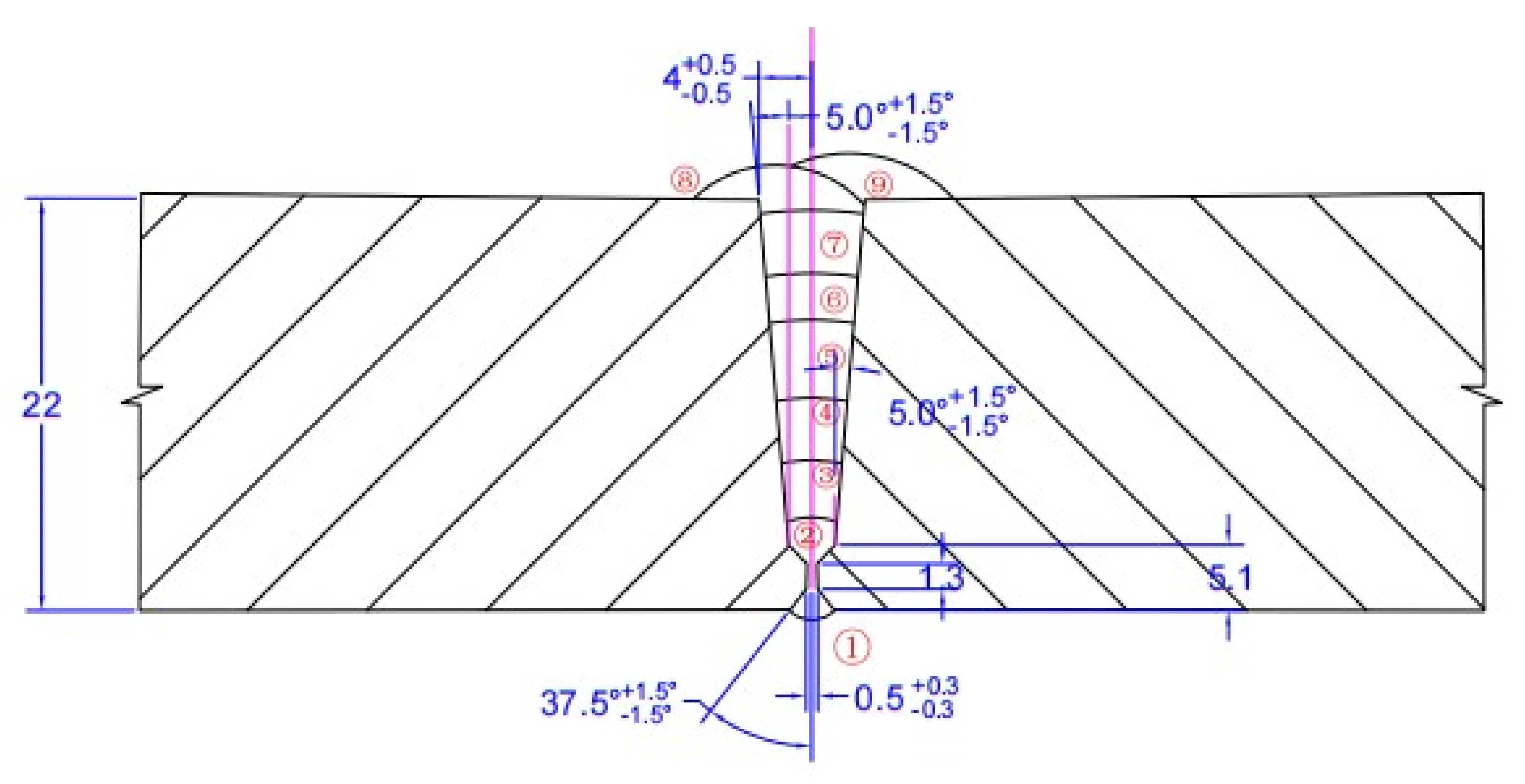
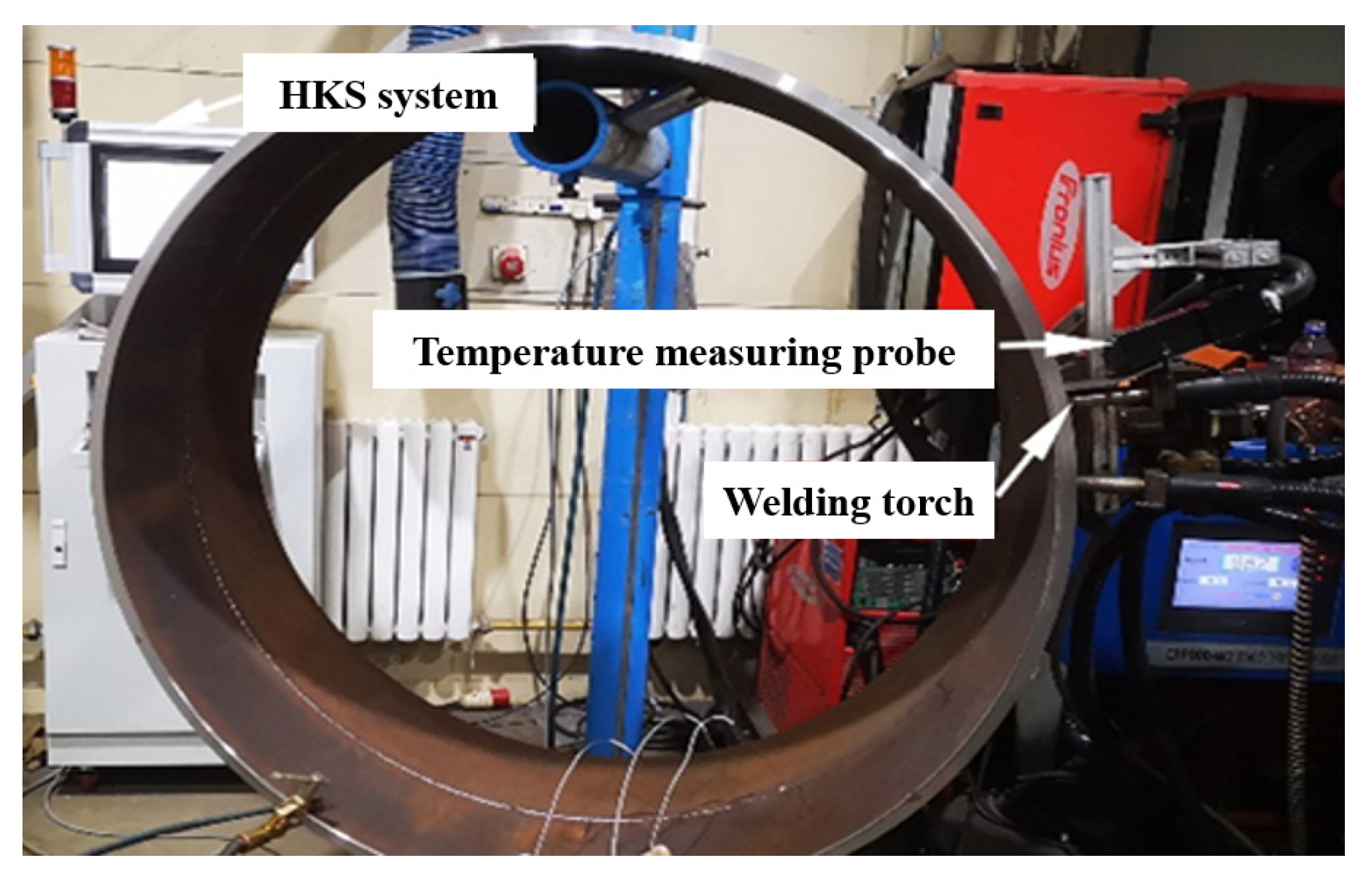
The experiment used X80M pipeline steel with a size of φ1219 × 22 mm, CPP900 as the welding power source, ASME SF A-5.28: ER80S-G solid welding wire with a diameter of 1 mm as the welding material, and a shielding gas of 80% Ar + 20% CO2. The diagram of groove and welds is shown in Figure 1, with 8 layers and 9 passes of welds. As shown in Figure 2, the HKS infrared system was used in the welding process to collect the temperature field 20 mm behind the welding gun, and the process parameters were recorded in real-time through the HKS data acquisition system. Considering that the incomplete fusion defects are mainly distributed at 4 to 6 o’clock positions, the experimental research area was selected at 3 to 6 o’clock positions, with a downwards vertical welding direction.

Figure 1.
Groove and weld profile (mm).
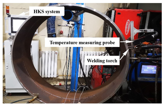
Figure 2.
Experiment and detection system.
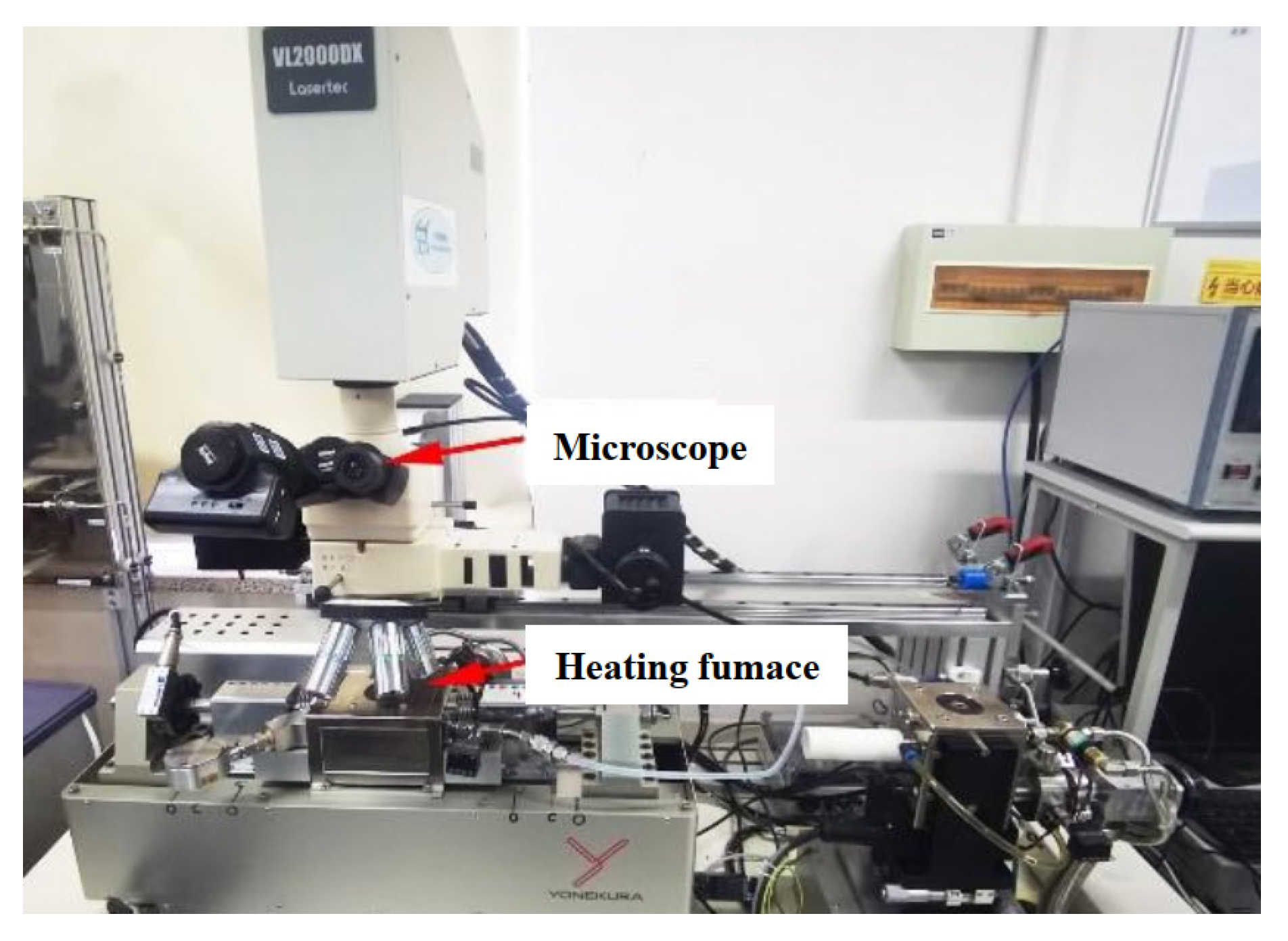
To conduct welding experiments and numerical simulation, the melting temperature of the material must be accurately measured. In this paper, an in situ laser confocal system with a heating table was used to heat the X80M sample, and the melting temperature of X80M was measured. The in situ observation system consists of a laser scanning confocal microscope and a high-temperature heating furnace, as shown in Figure 3.

Figure 3.
Laser confocal system.
3. Numerical Simulation and Swing Welding Model
3.1. Welding Heat Source Model
The heat source model can be regarded as a function of heat distribution in the time and space domains as the welding heat source acts on the weldment. It is the basis of numerical simulation to study the welding process, and a correct heat source model is crucial for the accuracy of the associated results. In this paper, a dynamic heat source model for the swing arc welding process was developed based on a dual-ellipsoidal heat source. It is self-coded with the FORTRAN language. The heat flux density distribution of the dual-ellipsoid heat source does not vary, but local coordinates of the heat source are changed according to the actual swing welding process. The heat flux distribution function of the dual-ellipsoid heat source is as follows:
where η is thermal efficiency; I is welding current; U is arc voltage; qr, qf are heat flux distribution functions of the front and rear parts of the heat source; and ar, af, bh, ch are shape coefficients of the heat source.
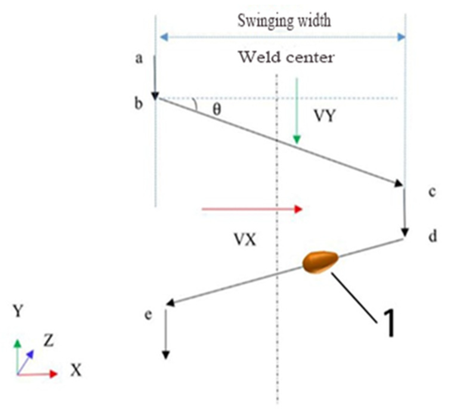
As shown in Figure 4, the moving speed of the welding gun can be decomposed into the moving speed along the welding direction (VY) and the swinging speed perpendicular to that direction (VX). By adjusting VY and VX, different swing frequencies and welding speeds can be realized. The swing welding trajectory can be divided into four stages:
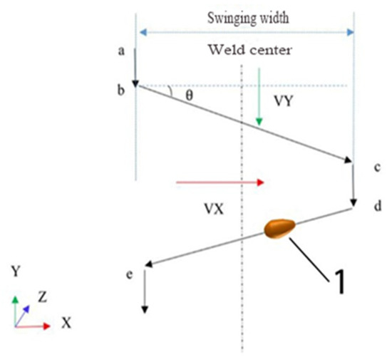
Figure 4.
Swing welding diagram.
- (1)
- The ab segment is the dwell stage on the left of the weld, in which VY is constant and VX is equal to 0;
- (2)
- The bc segment is the left-to-right swing stage, where VY remains unchanged, and VX is in the direction from left to right;
- (3)
- The cd segment maintains the constant VY, and VX is 0;
- (4)
- The de segment is the right-to-left swing stage, where the direction of VX is opposite to that in the bc segment.
3.2. Finite Element Model
Based on the Abaqus software, a finite element model of the automatic swing welding was constructed according to the actual long-distance pipeline, as shown in Figure 5. In order to ensure both the calculation efficiency and the accuracy, the mesh size near the weld and the heat-affected zone is 0.4 mm × 0.5 mm × 1 mm, and that far away from the weld zone is 2 mm × 2 mm × 1 mm. Considering the pipe diameter reaches 1219 mm, the temperature field far from the weld can be assumed to be independent of the welding structure. Therefore, the finite-sized model was enough to simulate the temperature field in the pipeline circular welding process. The weld morphology used in the finite element model is based on the metallographic morphology from experimental welded joints, which can take into account the effects of welding process, weld bead formation, external factors, etc.

Figure 5.
Finite element model of pipeline automatic swing welding.
3.3. Governing Equation and Boundary Conditions
The governing equation in the finite element model is expressed as follows [25]
where ρ is density, c is specific heat, k is thermal conductivity, T is temperature, t is time, and Q is a source term which includes heat source and latent heat of phase transition.
Heat radiation loss and heat convection loss act on the boundaries of the model, since the temperature is high in the welding process. Therefore, the integrated heat transfer coefficient is as follows:
where ε is the radiation emissivity; σ is the Boltzmann constant; T0 is the environment temperature; and hc is the convective heat transfer coefficient.
In the Abaqus software, the material is assumed to be composed of specific phases in certain proportions. The X80M involves several phases in the heating and cooling processes, including the FCC austenite phase and other BCC structure phases, such as ferrite phase, bainite phase, martensite phase, etc. The thermal conductivity and specific heat capacity of X80M are closely related to these phases. Figure 6 shows the thermal properties at different temperatures [26]. The Koistinen-Marburger (K-M) model was used for martensite transformations, which can be expressed as
where P is the proportion of martensite, T is temperature, Ms is martensite start temperature (445 °C), and b (0.01428) is the law parameter. Then, the total thermal conductivity and specific heat capacity can be calculated according to the volume fractions of austenite and other phases.

Figure 6.
Temperature- and phase-dependent parameters of the material: (a) thermal conductivity; (b) specific heat capacity.
4. Results and Discussion
4.1. Melting Point Analysis Based on In Situ Laser Confocal System
Incomplete fusion often occurs during welding processes, accompanied by “cold fusion” or “over fusion”. “Cold fusion” refers to a situation in which the melt of welding wire adjacent to the groove has a relatively low temperature, and it begins to solidify as soon as it reaches near the melting point temperature. The groove fails to fully melt due to the short duration of high-temperature conditions in the groove area, resulting in incomplete fusion, as depicted in Figure 7a. “Over fusion” refers to a situation in which the welding wire adjacent to the groove has a very high temperature and stays in the molten state for a long time, causing too much melting on the groove side, as shown in Figure 7b.
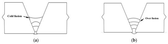
Figure 7.
Cold fusion and over-fusion defects: (a) cold fusion; (b) over-fusion.
An accurate evaluation of the melting temperature of X80M is helpful in determining the size of the molten pool in the simulation and evaluating the size of the melted region on the groove side, and it is crucial for defining the “cold fusion” or “over fusion” phenomenon. In this study, an in situ laser confocal system with a heating table was used to heat the sample at a rate of 13 °C/s until it was completely melted, and the melting point of the known material was accurately measured. In order to clearly observe the melting phenomenon of the X80M metallographic sample, the surface of the sample was mechanically polished without corrosion treatment, as shown in Figure 8a. When the sample was heated to 1560 °C, “pre-melting” or partial melting appeared on the coarse austenite grain boundaries (Figure 8b). When it was heated up to 1590 °C, most of the sample surface had melted (Figure 8c). Therefore, the melting temperature of X80M was defined as 1590 °C.

Figure 8.
Fusion test of X80M: (a) 25 °C; (b) 1560 °C; (c) 1590 °C.
4.2. Experimental Investigation of Pipeline Automatic Swing Welding
Welding process parameters in the pipeline automatic swing welding include welding current, welding voltage, welding speed, welding heat input, swing width, swing frequency, edge dwell time, etc. Previous experiments have shown that incomplete fusion mainly occurs at the 4 to 6 o’clock position and in the mode of sidewall incomplete fusion. Therefore, the welding experiment in this paper started from the 3 o’clock position and ended at the 6 o’clock position. During the experiment, the HKS system was used to collect the welding temperature field and related welding process parameters. Typical characteristics of pipeline automatic swing welding were investigated in the paper.
- (1)
- Welding process parameters
In order to reflect the characteristics used in the welding process, welding process parameters were recorded at 3, 4, 5, and 6 o’clock positions during the welding process. The heat input, welding speed, welding current, and swing width with welding positions were plotted in Figure 9. In accordance with the commonly used terms, welds ①, ②, ③, ④, ⑤, ⑥, ⑦, ⑧, and ⑨ were, respectively, recorded as root weld layer, hot weld layer, filling layer 1, filling layer 2, filling layer 3, filling layer 4, filling layer 5, covering weld 1, and covering weld 2.

Figure 9.
Welding process parameters of pipeline swing welding: (a) heat input at different positions; (b) welding speed at different positions; (c) welding current at different positions; (d) swing width at different positions.
In Figure 9a, it can be seen that the heat input of the hot weld layer is the smallest, and the heat input of filling layers 1, 2, 3, and 4 is similar, while the heat input of filling layer 5 differs greatly at different positions. The heat input of the hot weld layer and filling layers 1, 2, 3, and 4 are generally stable with the change of welding position. The heat input of filling layer 5 sharply decreases from position 4 to position 6.
In Figure 9b, it can be seen that the welding speed of each weld decreases gradually as the welding gun moves from 3 to 6 o’clock, and the welding speed of the hot weld layer is the fastest.
In Figure 9c, it can be seen that the welding current of each weld decreases gradually as the welding gun moves from 3 to 6 o’clock. Analysis shows that from position 3 to position 6, the welding position gradually changes from vertical welding to upward welding, and the effect of gravity on the molten pool becomes more and more significant. The current strategy ensures the stability of droplet transfer and weld pool by reducing welding speed and welding current while maintaining little change of heat input.
In Figure 9d, the swing width gradually increases as the welding gun moves from 3 to 6 o’clock. The growth rate is between 1.25 to 1.35 in the same filling layer. The welding mode changes from high-current rapid welding to low-current slow welding while the heat input is generally maintained at a stable level. However, the swing width between different filling layers varies a lot. Filling layers 1 and 2 have the same swing width, and filling layers 3 and 4 also have the same swing width, which is about 1.5 times that of the former, while filling layer 5 has the biggest swing width, which is almost 2 times that of filling layer 2. Appropriately increasing the swing width helps to increase the filling amount of the weld metal, increase the depth of the fusion zone, ensure the stability of welding droplets transfer and weld pool, and reduce the risk of incomplete fusion on the side wall.
- (2)
- Weld bead formation and incomplete fusion on sidewalls
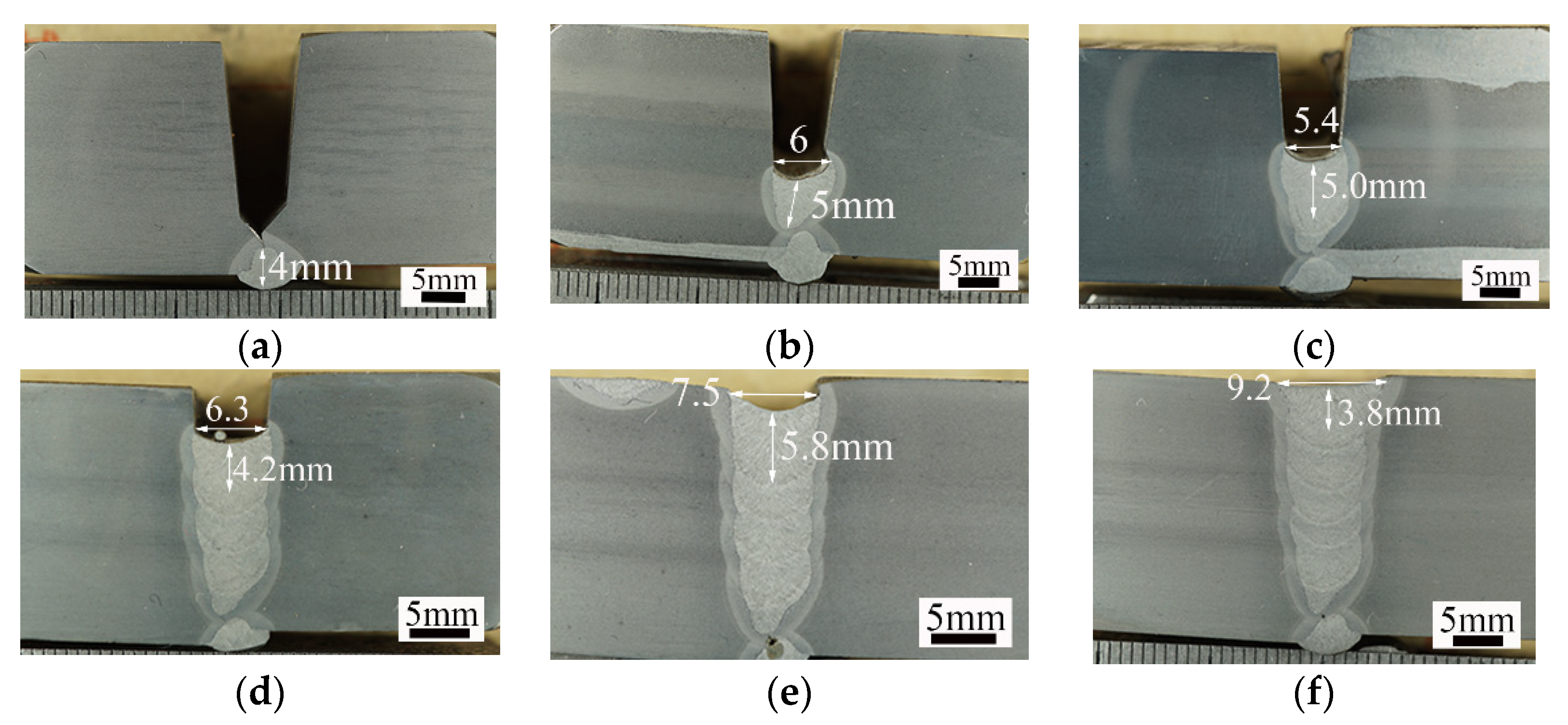
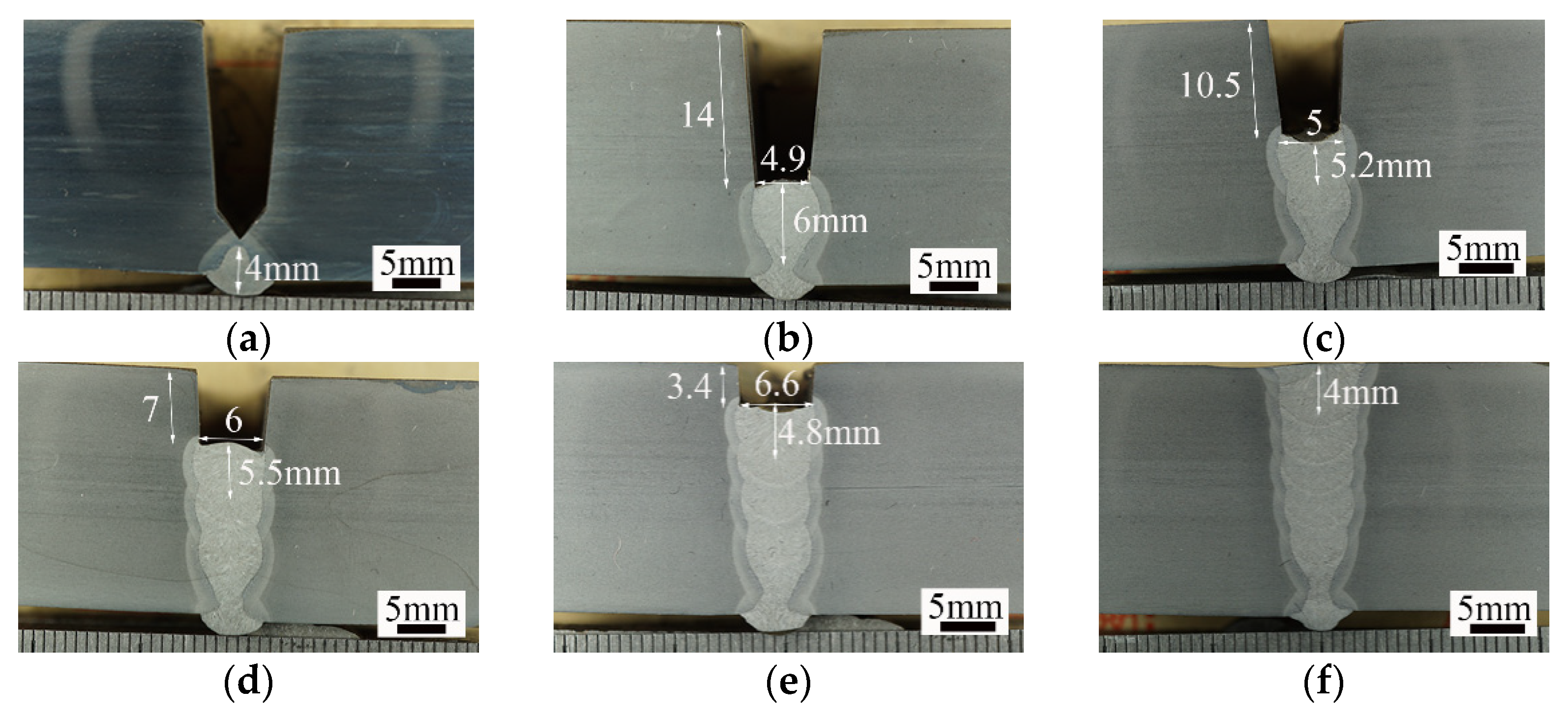
In order to investigate the relationship between weld bead formation and incomplete fusion defects, step-shaped welds were prepared at the 3 o’clock and 6 o’clock positions during the welding experiment. Therefore, the morphology of each weld can be observed and analyzed in detail. After welding, cross-sections of the step-shaped welds were taken and etched with a 4% nitric acid alcohol solution to display the weld profile. Figure 10 and Figure 11 show the morphology and size of different welds at the 3 o’clock and 6 o’clock positions, respectively. It shows that the welds at the 3 o’clock position have a “middle concave” morphology where the weld height near the groove wall is slightly higher than the middle weld due to the surface tension in the molten pool on both sides of the groove. This morphology can effectively avoid the occurrence of incomplete fusion on the sidewalls. On the other hand, the molten pool is more affected by gravity at the 6 o’clock position, resulting in a “hump” morphology on the hot weld layer and filling layer 3. When the “hump” morphology is more prominent, incomplete fusion on the sidewalls are more likely to occur. Therefore, the 6 o’clock position is more prone to sidewall incomplete fusion defects compared to the 3 o’clock position.
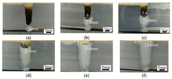
Figure 10.
Cross-section metallography of welding joint at 3 o’clock position: (a) root weld layer; (b) hot weld layer; (c) filling layer 1; (d) filling layer 3; (e) filling layer 4; (f) filling layer 5.
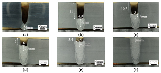
Figure 11.
Cross-section metallography of welding joint at 6 o’clock position: (a) root weld layer; (b) hot weld layer; (c) filling layer 1; (d) filling layer 3; (e) filling layer 4; (f) filling layer 5.
The above figure shows that the “hump” weld bead is more obvious in the hot weld layer and filling layer 3. By comparing the welding parameters, it can be found that the hot weld layer uses a straight-line welding technique without any swing, making it more susceptible to the influence of gravity and more likely to produce a “hump” weld bead. Additionally, filling layer 3 has a smaller swing width and lower welding current, causing it to be more prone to the formation of a “hump” weld bead.
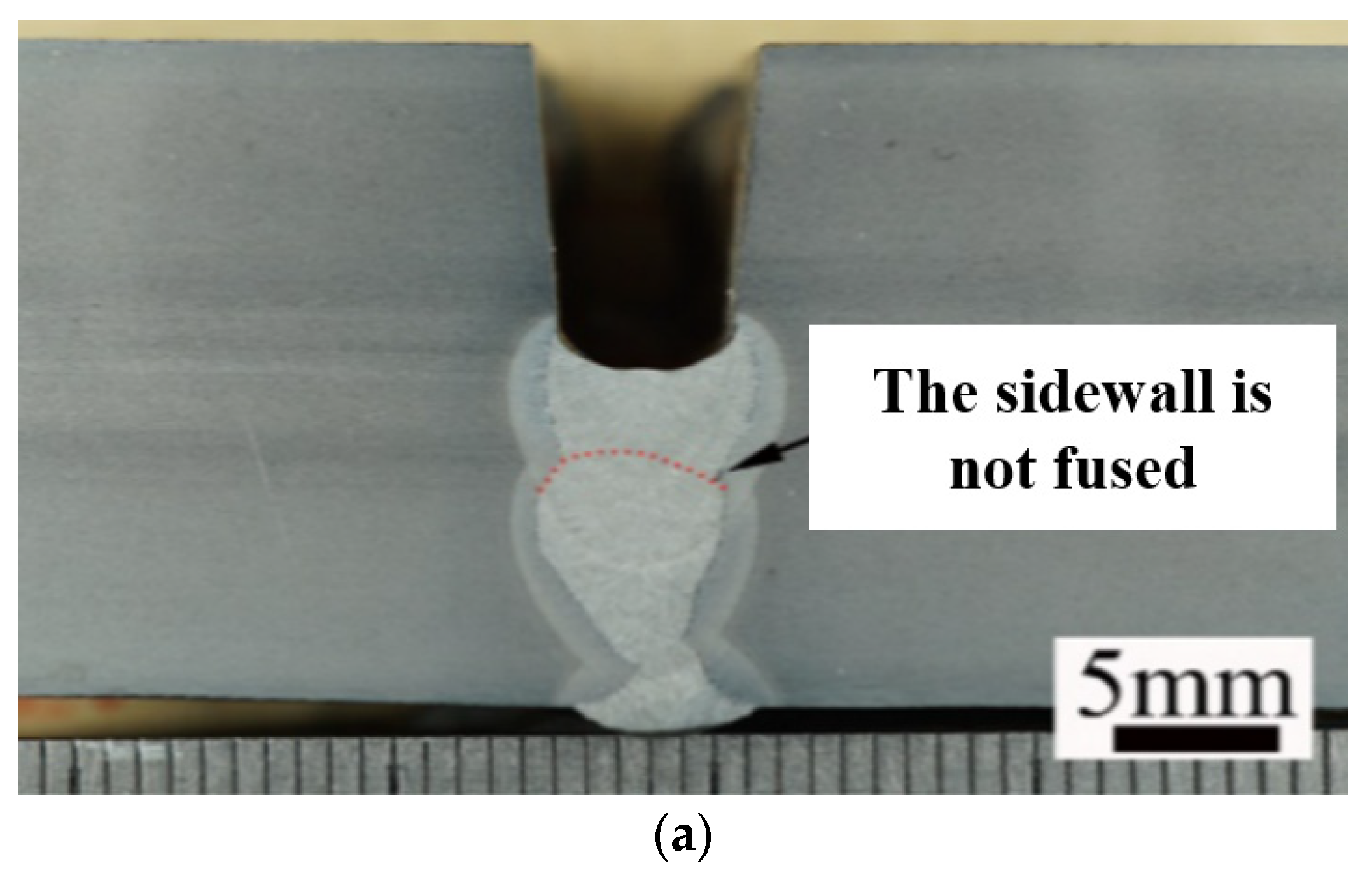
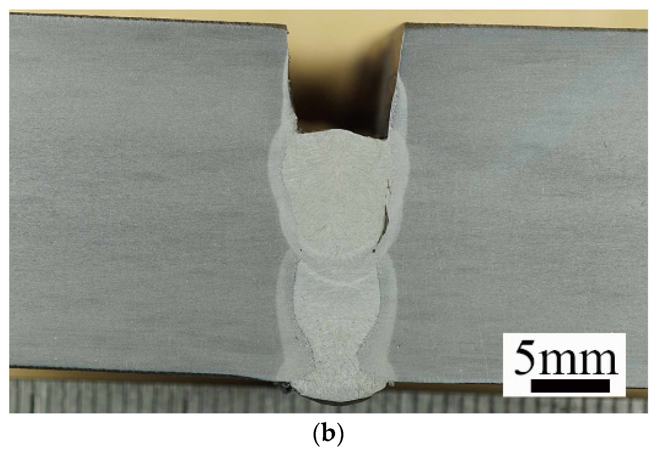
Figure 12 shows the incomplete fusion defects on the sidewall. They are considered to have a close relationship with the morphology of the current and next weld bead. If the current weld bead presents a typical “hump” morphology, the width of the current weld bead is generally small and the area near the groove edges cannot be fully melted. The “hump” morphology will affect the formation of the subsequent weld bead. If the next pass fails to eliminate the influence of the “hump”, incomplete fusion defects may occur on the side wall. Therefore, it is important to avoid the “hump” to prevent incomplete fusion defects. As discussed above, proper swing width is beneficial for the pipe welding process, as well as higher welding current.
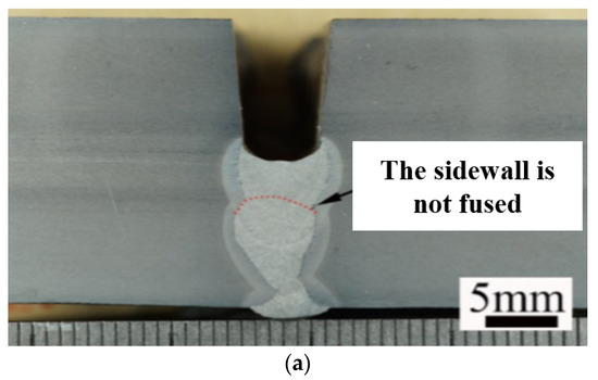
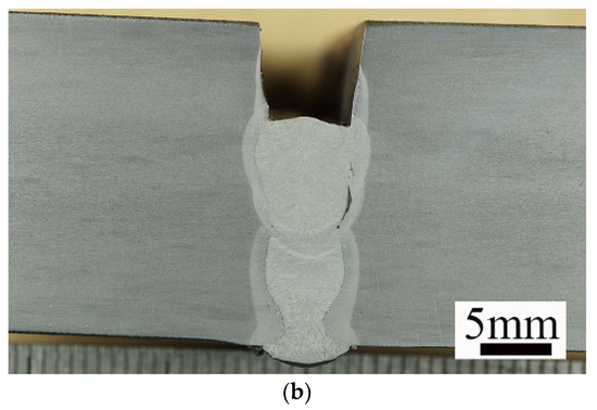
Figure 12.
Incomplete fusion defects on the sidewall: (a) incomplete fusion 1; (b) incomplete fusion 2.
- (3)
- Welding temperature field
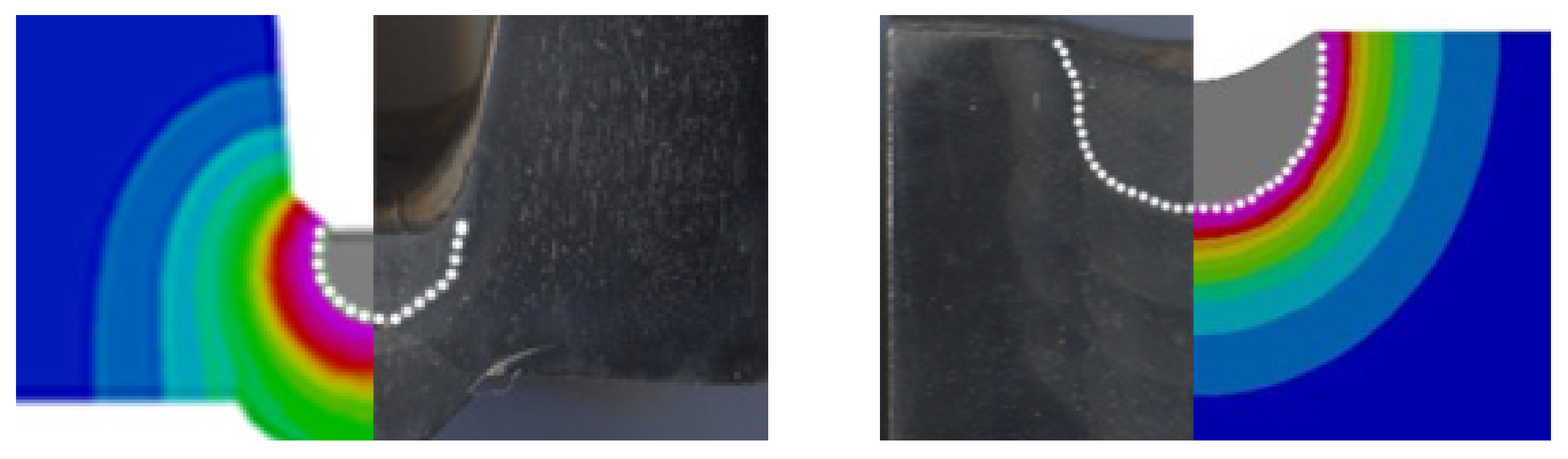
The selection of welding heat source is critical to ensure the accuracy of the simulation. The heat source model is usually validated by comparing the cross-section of the actual welding sample with the simulation result. Figure 13 demonstrates the comparison results of the vertical welding position. The simulation results are similar to the actual images, indicating that the heat source is appropriate in the simulation.

Figure 13.
Validation of the heat source model compared with the experimental results.
In the simulation, the heat source moved in the same way as in the actual swing welding process in Figure 4. When the heat source moves to the cd segment, the position is sufficiently heated, while the opposite be segment cannot be directly heated by the heat source. At the same time, the macroscopic temperature field shows that the temperature of the cd segment is higher than that of the be segment. The temperature field exhibits an asymmetric sawtooth distribution.
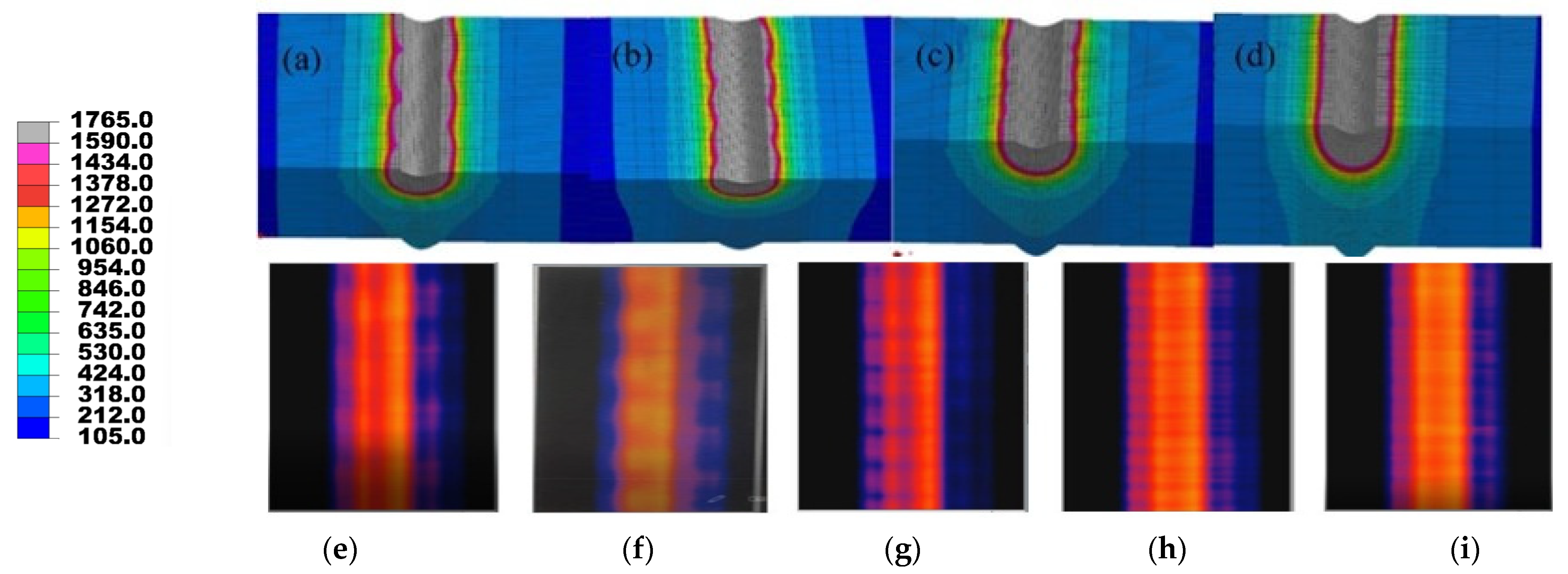
Figure 14 shows the temperature fields calculated by the model and measured by the HKS system, respectively. As mentioned earlier, the measured zone is located about 20 mm behind the welding wire, where is already solidified. The peak temperature in the zone is between 900–1200 °C, and the HKS system cannot directly measure the temperature within the molten pool. The numerical simulation can analyze the temperature field at any time and any location during the welding process, and it provides more detailed information regarding the weld pool than the experimental test. Figure 14 indicates that the temperature fields predicted by numerical simulation have similar distributions with that measured in the experiments. They both present an obvious “sawtooth” shape at small swing frequencies. The “sawtooth” shape can be gradually decreased by increasing the swing frequency, and it was effectively eliminated when the swing frequency reaches over 5 H.

Figure 14.
Temperature field at different swing frequencies ((a–d) simulation results, (e–i) experimental results): (a) 2 Hz; (b) 3 Hz; (c) 4 Hz; (d) 5 Hz s; (e) 2 Hz; (f) 3 Hz; (g) 4 Hz; (h) 5 Hz; (i) 6 Hz.
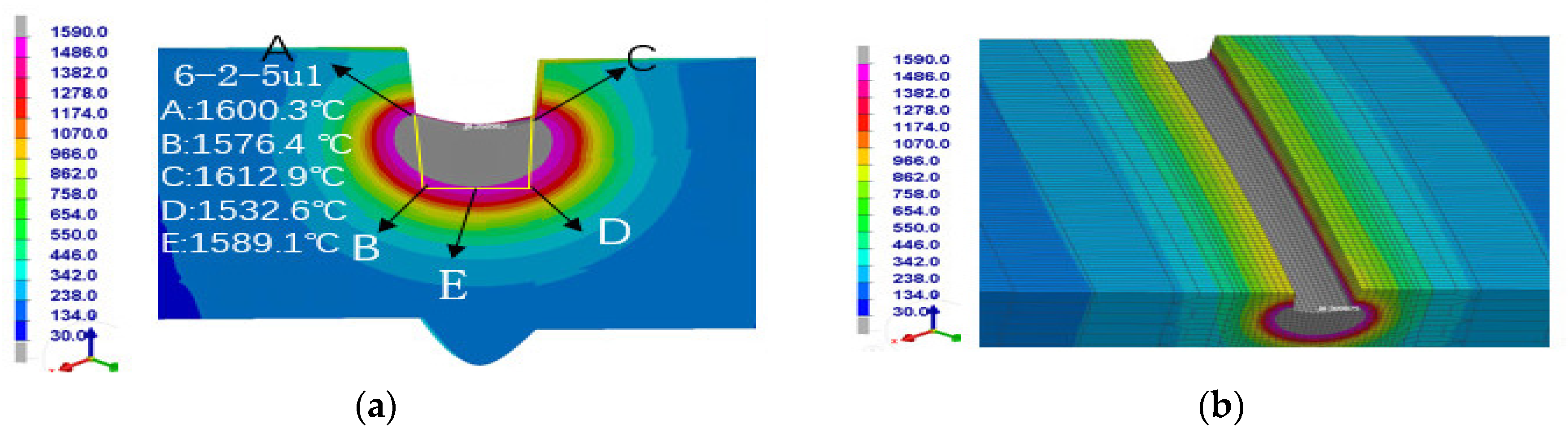
Further analysis of the cross-section temperature field in automatic swing welding illustrates that the temperature field in the inner and nearby regions of the groove is non-uniform during swing welding. As shown in Figure 15, the temperature at point A is lower than that at point C, while the temperature at point B, which is at the same side of point A, is higher than that at point D, which is at the same side of point C. This implies that the average temperature is generally balanced between AB side and CD side. Figure 15b displays a 3D temperature field of the weld bead, and the temperature distributions on the both sides are similar. Therefore, the swing strategy (frequency over 5 Hz) may help reduce the average temperature difference on both sides of the weld bead.
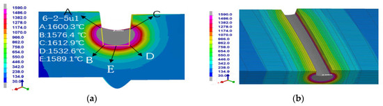
Figure 15.
Temperature field distribution due to the swing: (a) cross-section temperature field; (b) 3D temperature field.
5. Conclusions
This study conducted welding experiments and a numerical simulation to investigate the micro-swing welding process for X80M pipeline. A swing welding strategy was proposed according to the actual welding conditions of long-distance pipelines. The swing width grew to 1.25–1.35 times from the 3 to 6 o’clock position in the same filling layer. It also increases with filling layers, and filling layer 5 has the biggest swing width, which is almost two times that of filling layer 2. It was found that appropriately increasing the swing width helps to reduce the risk of incomplete fusion on the side wall.
“Middle concave” morphology appeared at the 3 o’clock position, which can effectively avoid the occurrence of incomplete fusion, while “hump” morphology may appear at the 6 o’clock position, and incomplete fusion defects will occur if the next pass fails to eliminate the influence of the “hump”. The 6 o’clock position is more prone to sidewall incomplete fusion defects compared to the 3 o’clock position.
A “Sawtooth” temperature field arose from the swing welding strategy. An obvious “sawtooth” shape appeared at small swing frequencies, and it was decreased by increasing the swing frequency. When the swing frequency reached over 5 Hz, it can be effectively eliminated. The swing strategy (frequency over 5 Hz) may help reduce the average temperature difference on both sides of the weld bead.
Author Contributions
Conceptualization, Z.L. and H.Z.; methodology, Z.L.; software, Y.L.; validation, Z.L. and P.W.; formal analysis, H.Z.; investigation, Y.L.; resources, Z.L. and H.Z.; data curation, P.W. and Y.L.; writing—original draft preparation, Y.L.; writing—review and editing, Z.L.; visualization, P.W. and Y.L.; supervision, Z.L.; project administration, Z.L.; funding acquisition, Z.L. and H.Z. All authors have read and agreed to the published version of the manuscript.
Funding
This research was funded by National Key R&D Program of China (Grant No. 2022YFC3070100) and National Natural Science Foundation of China (Grant No. 52076216).
Data Availability Statement
The data presented in this study are available on request from the corresponding author.
Conflicts of Interest
The authors declare no conflict of interest.
References
- Quan, T. Application Status and Prospect of Automatic Welding Technology for Long Distance Oil and Gas Pipelines in China. Nat. Gas Ind. 2021, 33, 69–70. [Google Scholar]
- Lu, Y.; Shao, Q.; Sui, Y.; Feng, D. Girth welding technology for large-diameter high steel grade gas line pipes. Nat. Gas Ind. 2020, 40, 114–122. [Google Scholar]
- Xu, Q.; Zhang, L.; Wu, D. Automatic Welding Technology for the Sino-Russian Eastern Route Gas Pipeline. Nat. Gas Technol. Econ. 2017, 11, 37–39. [Google Scholar]
- Zhang, X.; Jiang, Q.; Zhan, S.; Gu, Q.; Jin, J.; Wang, Q. Design improvement measures for the automatic welding of high-steel-grade and large-diameter gas line pipes in the project of the China–Russian Eastern Gas Pipeline. Nat. Gas Ind. 2020, 40, 126–132. [Google Scholar]
- Zhang, F.; Liu, X.; Xu, X.; Zhang, Y.; Niu, L. Study on the equipment and techniques for automatic pipeline welding in mountain area. Electr. Weld. Mach. 2018, 48, 37–41. [Google Scholar]
- Sun, L. Construction resource allocation and economy analysis of automatic welding for long -distance pipeline. Electr. Weld. Mach. 2021, 51, 95–100. [Google Scholar]
- Ren, G.; Zhang, X.; Guo, J. Comparative analysis of automatic welding process for all positions of long distance pipeline. Weld. Cut. 2018, 807, 42–44. [Google Scholar]
- Shen, H.; Chen, Z.; Feng, Z. Simulation of temperature field in automatic welding of oil and gas pipeline. Pet. Petrochem. Mater. Procure. 2021, 25, 53–55. [Google Scholar]
- Zong, X.; Wu, B.; Zhang, L.; Li, W. Numerical simulation of temperature field in weaving welding based on ladder model. Trans. China Weld. Inst. 2014, 35, 9–12. [Google Scholar]
- Zhang, H.; Zhang, G.; Cai, C.; Wang, J.; Wu, L. Numerical simulation on temperature field of dynamic welding processing with weaving. Trans. China Weld. Inst. 2008, 29, 69–76. [Google Scholar]
- Qi, Z.; Yang, X. Welding defects characteristics and prevention on metal-cored wire all-position pipe welding. Electr. Weld. Mach. 2012, 42, 84–86. [Google Scholar]
- Zhang, J.; Tang, D.; Zhang, T.; Hou, Z. Causes of Frequently Appeared Defects in Pipeline Automatic Welding and Preventive Measures. Pet. Eng. Constr. 2005, 31, 44–47. [Google Scholar]
- Rihar, G.; Uran, M. Lack of Fusion Characterisation of Indications. Weld. World 2006, 50, 35–39. [Google Scholar] [CrossRef]
- Lv, C.; Lei, Z.; Xia, S. Analysis and Treatment of Welding Defect in Narrow Gap Automatic Welding pf primary Coolant pipeline of ACP1000 Demonstration Project. China Nucl. Power 2020, 13, 148–154. [Google Scholar]
- Bandhu, D.; Djavanroodi, F.; Shaikshavali, G.; Vora, J.J.; Abhishek, K.; Thakur, A.; Kumari, S.; Saxena, K.K.; Ebrahimi, M.; Attarilar, S. Effect of Metal-Cored Filler Wire on Surface Morphology and Micro-Hardness of Regulated Metal Deposition Welded ASTM A387-Gr. 11-Cl. 2 Steel Plates. Materials 2022, 15, 6661. [Google Scholar] [CrossRef]
- Chen, Y.; Sun, S.; Zhang, T.; Zhou, X.; Li, S. Effects of post-weld heat treatment on the microstructure and mechanical properties of laser-welded NiTi/304SS joint with Ni filler. Mater. Sci. Eng. A 2020, 771, 138545. [Google Scholar] [CrossRef]
- Chen, Y.; Mao, Y.; Lu, W.; Peng, H. Investigation of welding crack in micro laser welded NiTiNb shape memory alloy and Ti6Al4V alloy dissimilar metals joints. Opt. Laser Technol. 2017, 91, 197–202. [Google Scholar]
- Zhang, Z.; Shao, C. Numerical simulation and visualization experiment of gas-liquid two phase flow in the centrifugal pump. J. Nanjing Tech Univ. (Nat. Sci. Ed.) 2020, 13, 148–154. [Google Scholar]
- Wang, G.; Jia, L.; Zhang, X. CFD numerical simulation of pulse-jet cleaning efficiency based on response surface method. J. Nanjing Tech Univ. (Nat. Sci. Ed.) 2022, 44, 132–140. [Google Scholar]
- Zhu, C.; Cheon, J.; Tang, X.; Na, S.-J.; Lu, F.; Cui, H. Effect of swing arc on molten pool behaviors in narrow-gap GMAW of 5083 Al-alloy. J. Mater. Process. Technol. 2018, 259, 243–258. [Google Scholar] [CrossRef]
- Xu, G.; Wang, J.; Li, P.; Zhu, J.; Cao, Q. Numerical analysis of heat transfer and fluid flow in swing arc narrow gap GMA welding. J. Mater. Process. Technol. 2017, 252, 260–269. [Google Scholar] [CrossRef]
- Panwisawas, C.; Sovani, Y.; Turner, R.P.; Brooks, J.W.; Basoalto, H.C.; Choquet, I. Modelling of thermal fluid dynamics for fusion welding. J. Mater. Process. Technol. 2017, 252, 176–182. [Google Scholar] [CrossRef]
- Yang, T.; Liu, J.F.; Zhang, Y.; Sun, K.; Chen, W. Studies on the formation mechanism of incomplete fusion defects in ultra-narrow gap laser wire filling welding. Opt. Laser Technol. 2020, 129, 1–7. [Google Scholar] [CrossRef]
- Wang, H.; Li, X.; Zhang, B.; Liu, X.; Yan, H.; Wang, Z. Technology of causes and suppression of weld edge incomplete fusion for long-distance pipeline automatic welding. Electr. Weld. Mach. 2019, 49, 57–61. [Google Scholar]
- Zhao, W.; Jiang, W.; Zhang, H.; Han, B.; Jin, H.; Gao, Q. 3D finite element analysis and optimization of welding residual stress in the girth joints of X80 steel pipeline. J. Manuf. Process. 2021, 66, 166–178. [Google Scholar] [CrossRef]
- Zhang, H.; Wang, Y.; Han, T.; Bao, L.; Wu, Q.; Gu, S. Numerical and experimental investigation of the formation mechanism and the distribution of the welding residual stress induced by the hybrid laser arc welding of AH36 steel in a butt joint configuration. J. Manuf. Process. 2020, 51, 95–108. [Google Scholar] [CrossRef]

Disclaimer/Publisher’s Note: The statements, opinions and data contained in all publications are solely those of the individual author(s) and contributor(s) and not of MDPI and/or the editor(s). MDPI and/or the editor(s) disclaim responsibility for any injury to people or property resulting from any ideas, methods, instructions or products referred to in the content. |
© 2023 by the authors. Licensee MDPI, Basel, Switzerland. This article is an open access article distributed under the terms and conditions of the Creative Commons Attribution (CC BY) license (https://creativecommons.org/licenses/by/4.0/).