Numerical Simulation of Magnetic Field and Flow Field of Slab under Composite Magnetic Field

Abstract

A kind of composite magnetic field for flow control in slab mold is proposed, in which an electromagnetic stirring (EMS) is carried out near the meniscus and an electromagnetic braking (EMBr) is carried out near the outlet of the submerged entry nozzle (SEN), simultaneously. The yoke for the EMS and the EMBr is made independent from each other, with a ruler type for the EMBr. A three-dimensional model of the magnetic field calculation is established. The simulation results show that the magnetic induction intensity generated with the EMS mainly concentrates in the EMS area. The magnetic induction intensity generated with the EMBr has a large component in the EMS results, which has little effect on the flow of this area. Based on the composite magnetic field calculation results, the three-dimensional numerical simulation of the flow field is carried out, and the flow field obtained is compared to that without the magnetic field but with the EMS and the EMBr only, respectively. The results show that under the composite magnetic field, EMBr and EMS can play their respective roles well under certain conditions, the impact of the jet flow on the narrow face is reduced, and the stirring beneath the meniscus is intensified.

1. Introduction

With the development of continuous casting technology, higher-quality slab production became a common goal of steel enterprises. Flow in the slab mold is essential to the quality [1]. At present, the main technologies to control the flow behavior in the mold are EMBr technology and EMS technology [2,3,4,5,6]. EMS in slab mold is used to activate the flow near the meniscus, which can improve the equiaxed grain ratio, scour the solidification front, and reduce the non-metallic inclusions in the liquid–solid interface [7,8,9,10,11]; however, EMS can neither reduce the impact of the jet flow from the SEN on the narrow face nor suppress the impinging depth of the downward flow. EMBr can reduce the impact of the jet flow on the narrow face of the mold [12,13,14,15,16]; however, a highly strong EMBr dulls the melting of the protective slag [17,18,19,20,21]. In order to solve the above problems, ABB in Sweden proposed the composite control technology of the flow field in slab mold with EMS and EMBr, simultaneously [22], but did not publish the specific scheme of magnet coil structure and magnetic field distribution. Song-Woo H et al. [23] combined a traveling magnetic field and a static magnetic field to study their control effect on the flow field and conducted a commercial plant test. In the test, the slab mold width was 2 m, and the casting speed was 0.95 m/min. The results reveal that the downward flow is reduced and that the rotation flow in the upper coil center is improved. However, in this research, an integral magnetic yoke was used, with which independent control of the EMS and the EMBr was relatively complicated. Sun et al. [24] employed a transient numerical model combined with the volume of fluid approach to study the effect of multifunction electromagnetic driving (also the combination of the EMS and the EMBr) on the steel/slag interface behavior. The results show that the multifunction electromagnetic ensures the uniformity of the molten steel in the upper region of the mold and that the distribution of surface velocity is more uniformed. In this research, a local-type EMBr was adopted, which could merely affect the flow adjacent to the SEN outlet.

In this paper, a kind of composite magnetic field for the flow control of slab mold is proposed in which the yoke is divided into two independent parts for EMS and EMBr, respectively. The magnetic field is composed of a linear traveling EMS near the meniscus and a ruler-type EMBr near the SEN outlet, forming a composite control of the flow field of the mold. The ruler-type EMBr can improve the flow near the whole wide face in the mold. A three-dimensional model of the magnetic field calculation is established, and the numerical simulation of the three-dimensional flow field of the molten steel in the mold under the composite magnetic field is carried out. The simulation result is also verified using a 1:4 model experiment. At present, steel grades such as automobile plates and household appliance plates have higher requirements on the quality of billets, and ordinary electromagnetic technology can no longer meet the flow control requirements of such steel grades. Therefore, composite magnetic fields are supposed to be used for this kind of steel, and the casting speed range for the large-width slab in the references is about 0.9–1.2 m/s [23,24] at present.

2. Mathematical Modeling

In order to better describe the flow of molten steel in the slab continuous casting mold under the composite magnetic field, the following assumptions were Pmade on the premise that the simulation results were reasonable.

In the calculation of the electromagnetic field, the influence of molten steel flow on the magnetic field was not considered since the magnetic Reynolds number was much less than one, as calculated later; the molten steel, copper coil, and yoke had constant physical and isotropic electromagnetic characteristics, and the displacement current was ignored. In the calculation of the flow field, the flow of molten steel in the mold was considered as steady, and the molten steel was an incompressible Newtonian fluid. The influence of mold vibration and taper on the flow field was not considered; the influence of solidified shell thickness was also not considered. The magnetic Reynolds number is R_m = μ_mσ vL ≈ 0.065 << 1, where v is the characteristic velocity of the molten steel (2.02 m/s), L is the characteristic length of the SEN (0.0325 m), μ_m is the magnetic permeability of molten steel (1.4 × 10⁻⁶ H/m), and σ is the electrical conductivity of molten steel (7.14 × 10⁵ S/m); this meant that the convection terms of the magnetic field could be neglected.

2.1. Electromagnetic Force Equations

The calculation of the composite magnetic field was divided into two parts, alternating the magnetic field and the static magnetic field. Electromagnetic field analysis was conducted by solving Maxwell’s equations and Ohm’s Law:

$$\nabla \cdot \overrightarrow{B}=0$$

(1)

$$\nabla \times {\overrightarrow{H}}_M=\overrightarrow{J}$$

(2)

$$\nabla \times \overrightarrow{E}=-\frac{\partial \overrightarrow{B}}{\partial t}$$

(3)

$$\overrightarrow{J}=\sigma \left(\overrightarrow{E}+\overrightarrow{U}\times \overrightarrow{B}\right)$$

(4)

$\overrightarrow{B}$ represents the magnetic flux density (T), ${\overrightarrow{H}}_M$ is the magnetic field intensity (Wb/A), $\overrightarrow{E}$ is the electric field intensity (N/C), $\overrightarrow{J}$ is the inductive current density (A/m²), t is the time (s), and $\sigma$ is the electrical conductivity (Ω⁻¹ ).

The eddy current solver was used to calculate the EMS part. The Lorentz force was expressed as a complex number, and the time average form could be obtained. The time average electromagnetic force can be expressed as follows:

$${\overrightarrow{F}}_{EMS}=\frac{1}{2}\mathrm{Re}(\overrightarrow{J}\times {\overrightarrow{B}}^{\ast })$$

(5)

where ${\overrightarrow{F}}_{EMS}$ is the electromagnetic stirring force (N/m³), ${\overrightarrow{B}}^{\ast }$ is the conjugate complex of $\overrightarrow{B}$(T), and $\mathrm{Re}$ is the real part of a complex number.

The static magnetic field solver was used in the calculation of the EMBr part, and the Lorentz force was obtained in the calculation of the flow field. The induced current and the electromagnetic force derived from Ohm’s law and Maxwell’s equation were calculated using the magnetic induction method [1]. The electromagnetic braking force can be expressed as follows:

$${\overrightarrow{F}}_{EMBr}=\overrightarrow{J}\times {\overrightarrow{B}}_0$$

(6)

Here, ${\overrightarrow{F}}_{EMBr}$ is the electromagnetic braking force (N/m³), ${\overrightarrow{B}}_0$ is the external DC magnetic field (T), and the magnetic flux density $\overrightarrow{B}$ is composed of the applied DC magnetic field ${\overrightarrow{B}}_0$ and the induced magnetic field $\overrightarrow{b}$ caused by cutting magnetic induction line of molten steel.

2.2. Turbulence Model

The governing equations for the three-dimensional incompressible fluid flow are described as follows:

$$\frac{\partial \rho }{\partial t}+\frac{\partial \rho u_i}{\partial x_i}=0$$

(7)

$$\frac{\partial \left(\rho u_i\right)}{\partial t}+\frac{\partial \left(\rho u_i{u}_j\right)}{\partial x_j}=-\frac{\partial p}{\partial x_i}+\frac{\partial }{\partial x_j}\left[{\mu }_{eff}\left(\frac{\partial u_i}{\partial x_j}+\frac{\partial u_j}{\partial x_i}\right)\right]+\rho g_i+F_i$$

(8)

$${\mu }_{eff}=\mu +{\mu }_t=\mu +\rho C_{\mu }\frac{k^2}{\epsilon }$$

(9)

where $\rho$ is the fluid density (kg/m³); u_i represents the velocity in the x, y, and z directions (represented by i, j = 1, 2, 3, respectively) (m/s); p is pressure (Pa); μ is the dynamic viscosity (Pa·s); F_i is the electromagnetic force (N/m³); $g_i$ is the gravitational acceleration (9.81 m/s²); ${\mu }_{eff}$ is the effective viscosity (kg·m⁻¹·s ⁻¹); $\mu$ and ${\mu }_t$ are the laminar and the turbulent viscosity coefficients (kg·m⁻¹·s ⁻¹); and $C_{\mu }$ is a constant.

The standard $k$-$\epsilon$ turbulence model [25] was used to solve the turbulent viscosity coefficient μ, the turbulent kinetic energy k, and the turbulent dissipation rate $\epsilon$, as follows:

$$\frac{\partial }{\partial t}(\rho k)+\frac{\partial }{\partial x_i}(\rho k{u}_i)=\frac{\partial }{\partial x_i}\left[\left(\mu +\frac{{\mu }_t}{{\sigma }_k}\right)\frac{\partial k}{\partial x_j}\right]+G_k-\rho \epsilon$$

(10)

$$\frac{\partial }{\partial t}(\rho \epsilon )+\frac{\partial }{\partial x_i}(\rho \epsilon u_i)=\frac{\partial }{\partial x_j}\left[\left(\mu +\frac{{\mu }_t}{{\sigma }_k}\right)\frac{\partial \epsilon }{\partial x_j}\right]+C_{1\epsilon }\frac{\epsilon }{k}{G}_k-C_{2\epsilon }\rho \frac{{\epsilon }^2}{k}$$

(11)

G_k represents the generation of turbulence kinetic energy due to the mean velocity gradients:

$$G_k=-\rho \overline{u_i^{\prime }{u}_j^{\prime }}\frac{\partial u_j}{\partial x_i}$$

(12)

The model constants $C_{1\epsilon }$, $C_{2\epsilon }$, $C_{\mu }$, ${\sigma }_k$, and ${\sigma }_{\epsilon }$ have the following default values: $C_{1\epsilon }$ = 1.44, $C_{2\epsilon }$ = 1.92, $C_{\mu }$ = 0.09, ${\sigma }_k$ = 1.0, and ${\sigma }_{\epsilon }$ = 1.3.

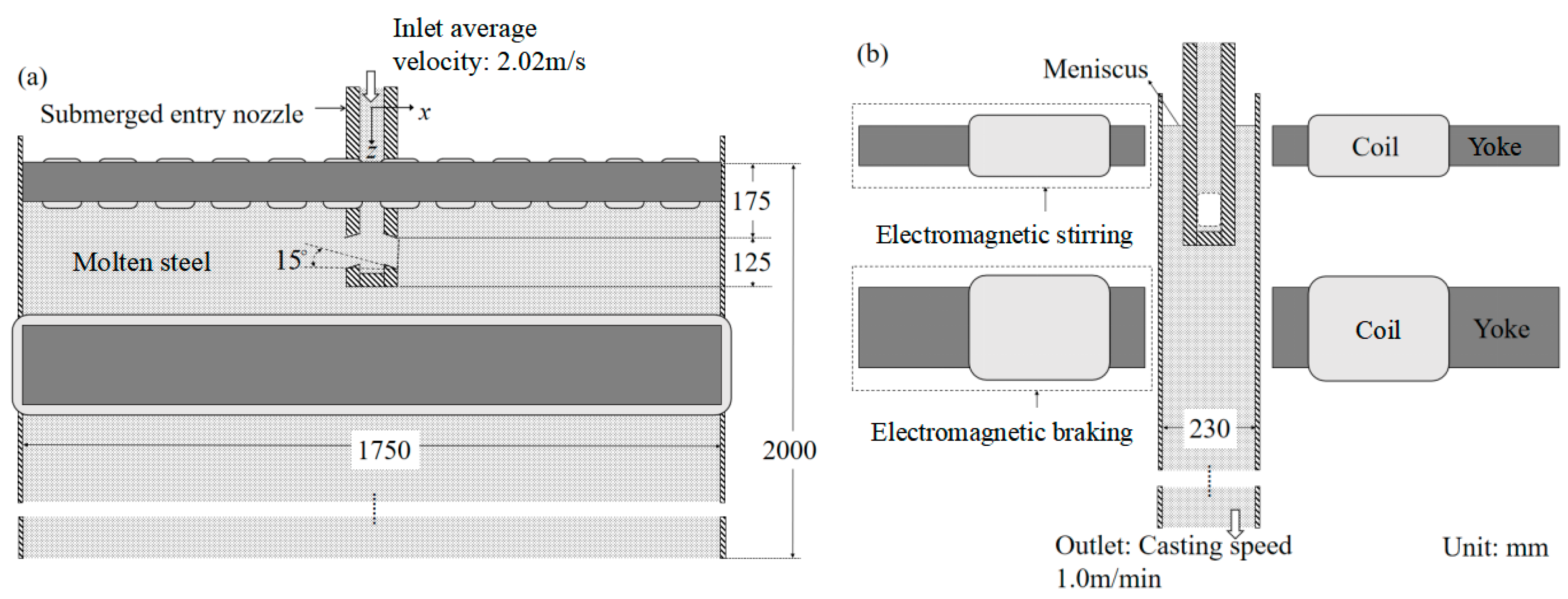
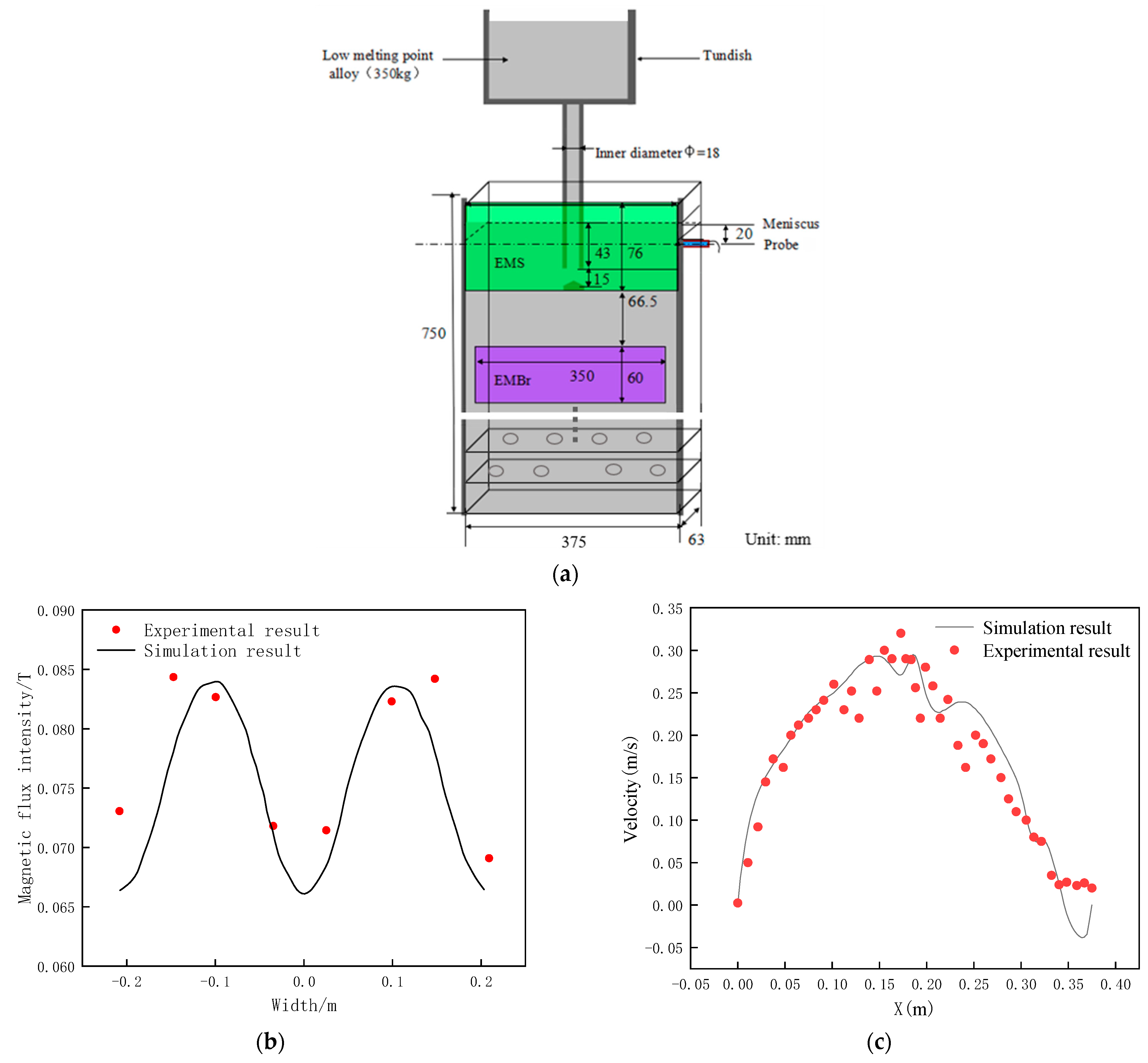
2.3. Mesh and Boundary Conditions

The mesh of the computational domain for the magnetic field shown in Figure 1a was tetrahedral. The number of grid nodes reached 1 million, the maximum length of the grid was 25 mm, and the minimum was 1 mm. The calculated residual of the magnetic field was 10⁻⁸. Since F_EMS was calculated using Equation (5), the calculated residual for the F_EMS is the same as that in the magnetic field calculation. F_EMBr was calculated using Equation (6), and the calculated residual for the F_EMBr was decided with the calculation residual for the flow fluid calculation, which will be given in Section 2.4. The whole device was surrounded by the air region, and the air region surface was provided with the parallel boundary conditions of the magnetic lines.

2.4. Calculation Process

The calculation of the composite magnetic field was divided into two parts: EMBr and EMS. The data of magnetic induction intensity in the mold under EMBr were derived in commercial software and loaded into the MHD module in Fluent with the help of MATLAB language. Here, the magnetic calculation result was obtained using the finite difference method, and the result data pattern could be transferred with the MATLAB to the pattern that could be recognized using the MHD module in Fluent, which used the finite volume method. The time average electromagnetic force in the mold under EMS was derived in commercial software and loaded into the flow field calculation through UDF function [24].

The mesh of the computational domain for flow field shown in Figure 1b was hexahedral. The number of the grid of the hexahedral cells was about 0.67 million. The maximum volume was 0.49 × 10⁻⁶ m³ and the minimum was 0.16 × 10⁻⁷ m³, which met the requirements of the Fluent [26]. The velocity inlet was at the SEN inlet, with outflow at the outlet, no slip boundary condition at the mold wall, and zero shear wall at the meniscus. When the residual of the calculated mass is less than 10⁻³ and the residual of the turbulent kinetic energy is less than 10⁻³, it is considered that the calculation of the flow field converges.

The structure of the composite magnetic field is shown in Figure 2. The parameters for calculating magnetic field and flow field are given in

Table 1. Model for structural, physical, and operational parameters.

Parameters	Values
Domain width	1750 mm
Domain length	3000 mm
Domain thickness	230 mm
Molten steel conductivity	7.14 × 105 S/m
Coil electric conductivity	6.25 × 107 S/m
Molten steel density	7020 kg/m3
Molten steel viscosity	0.0062 kg/m·s
Casting speed	1.0 m/min
SEN submerged depth	300 mm
EMS current intensity	150 A
EMBr current intensity	240 A
AC frequency	4 Hz

.

3. Results

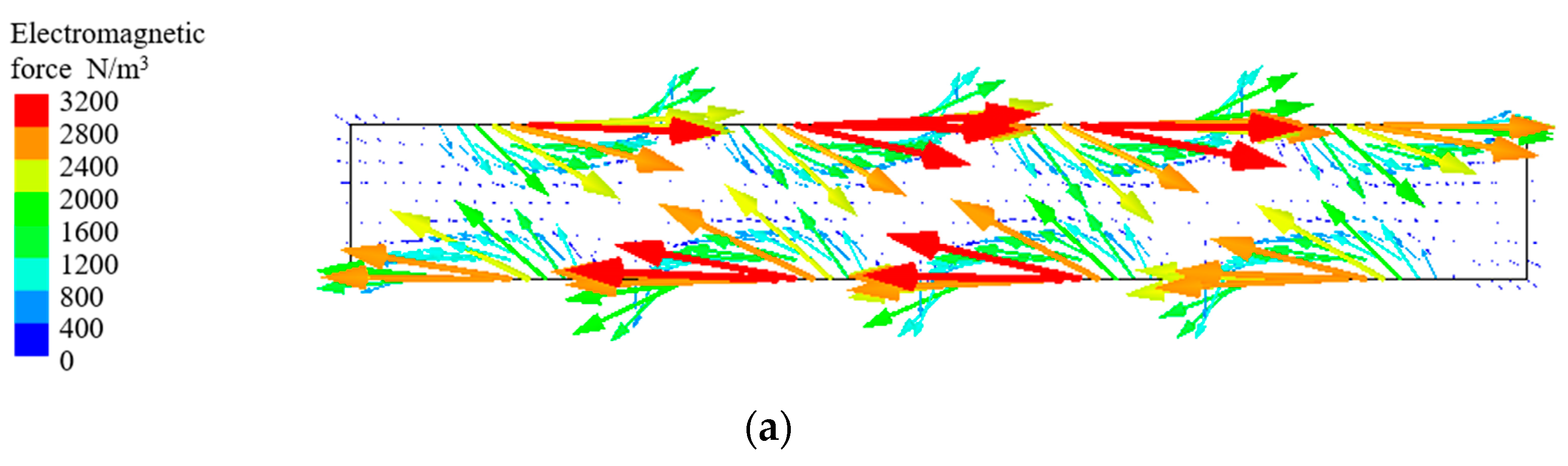
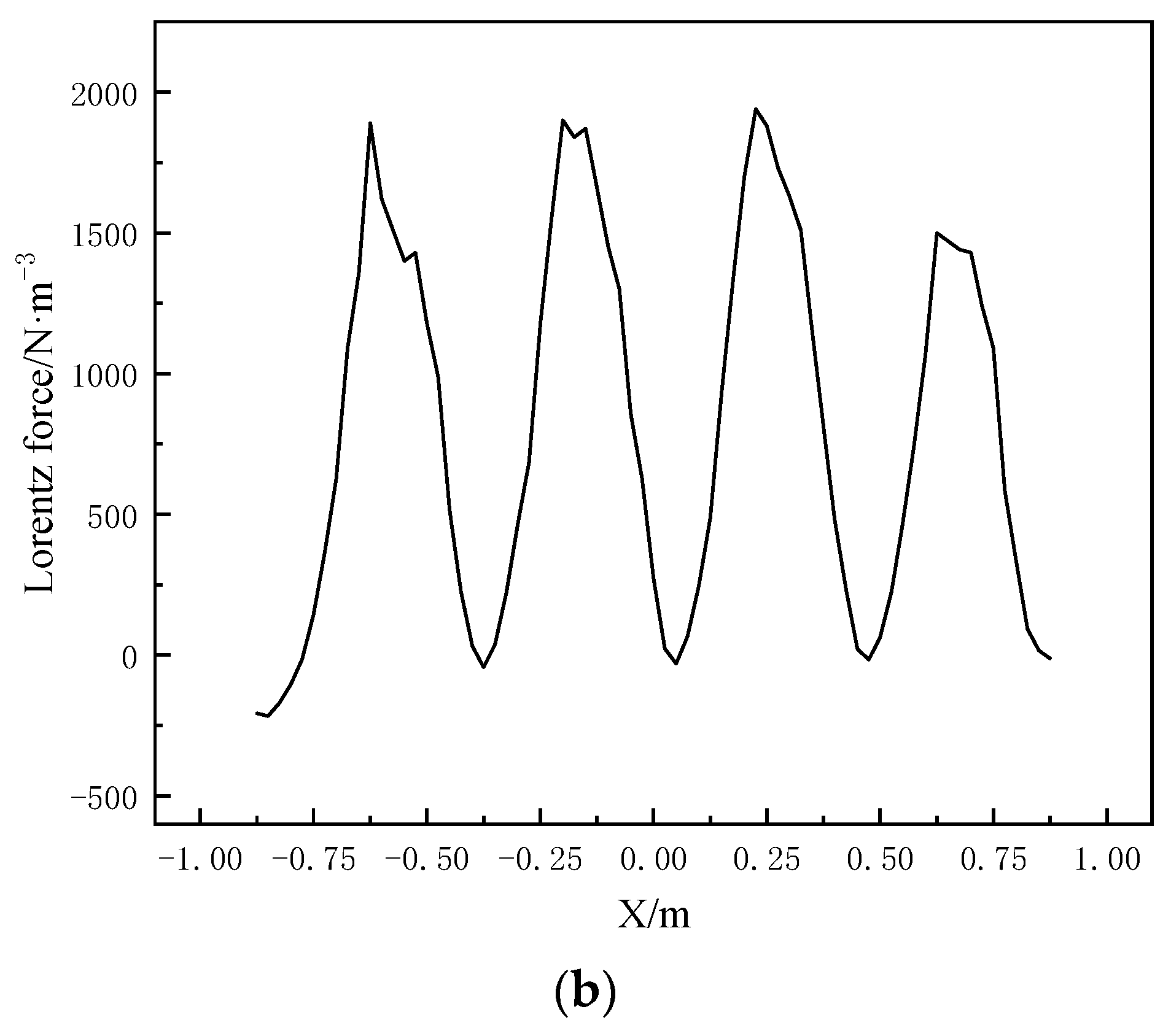
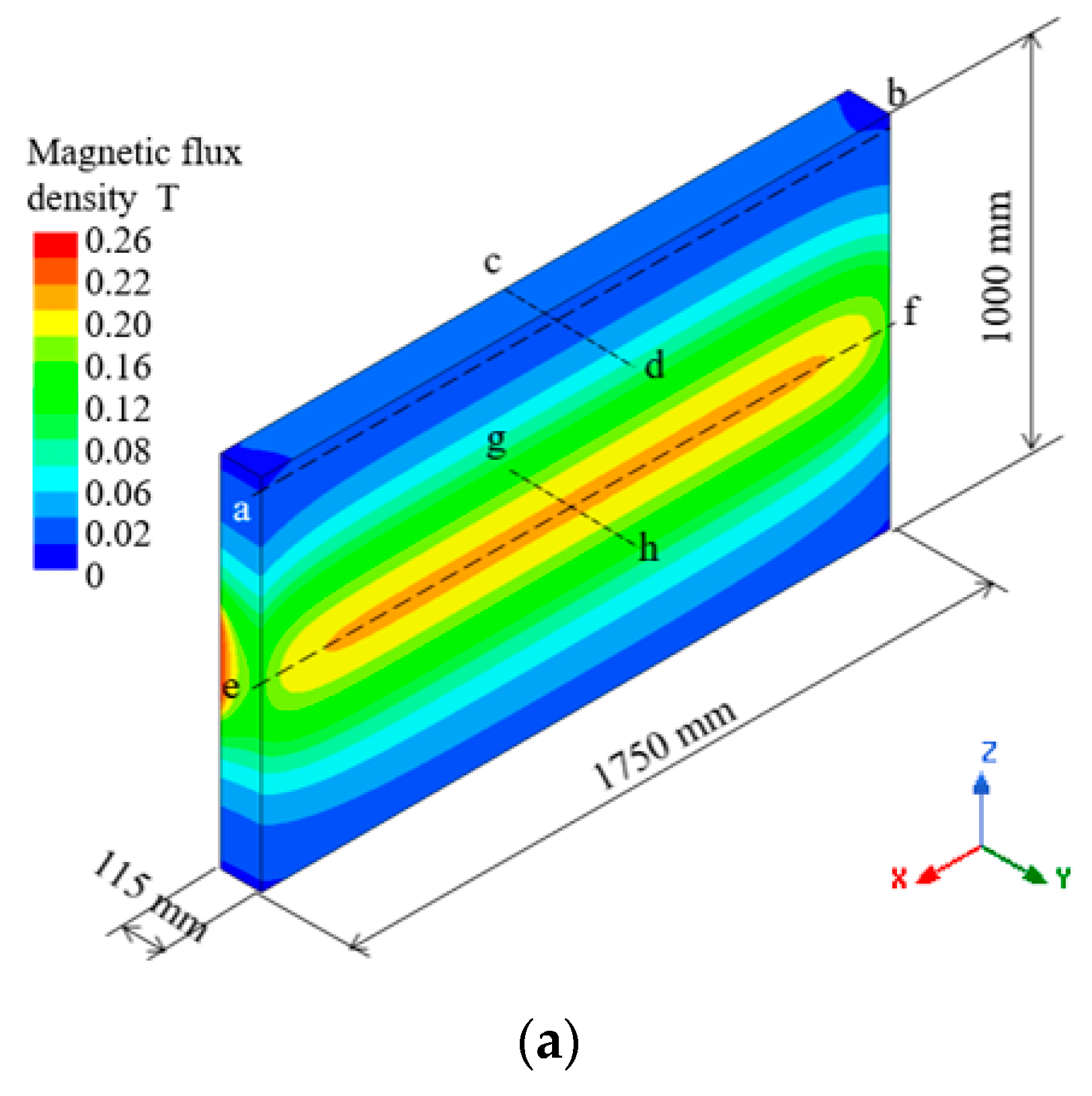
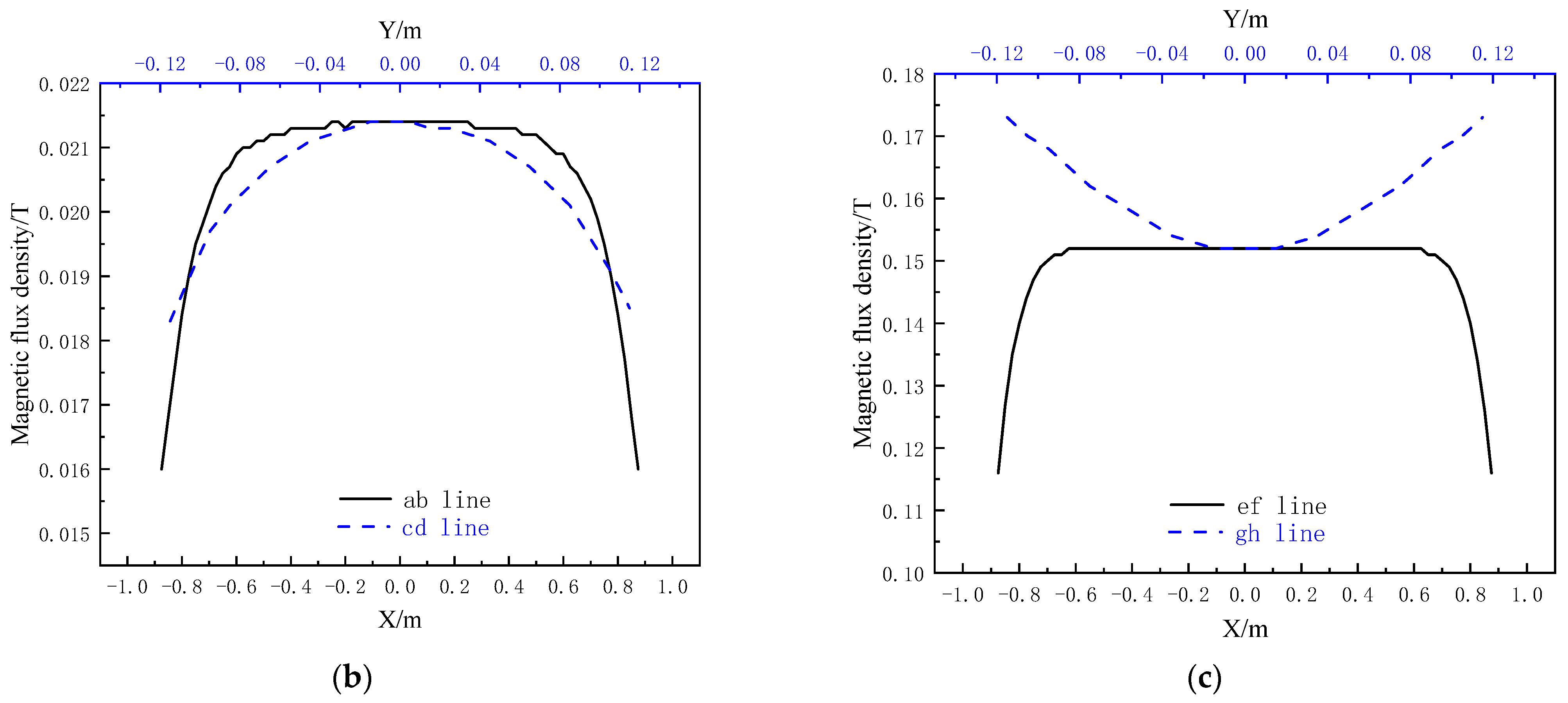
3.1. Electromagnetic Field Simulation

In Figure 3a, it shows the contour plot of the magnetic flux density in the mold under EMS only, while Figure 3b,c show the distribution of magnetic flux density at different lines in the mold. The ab and cd are horizontal center lines of the EMS central region in the wide side and the narrow side, respectively; the ef and gh are horizontal center lines of the EMBr central region in the wide side and the narrow side. The results in the cd line and gh line in the figures correspond to upper abscissa of the figures. There are four wave peaks of magnetic flux density in the ab line. This is because there are 12 yokes on each side of the EMS device. Every three yokes are one group. In total, there are four groups; therefore, four wave peaks will be generated. The magnetic flux density can be found as the largest on the mold wall. In the EMS area, the magnitude of magnetic flux density is in the order of 10⁻² T, but in the EMBr area, the magnitude of magnetic flux density is only in the order of 10⁻³ T, which is much weaker than that produced with the EMBr only in this area (order of 10⁻¹ T as shown later in Figure 3c). Therefore, the magnetic flux density produced with the EMS affects little on the magnetic field and thus on the flow field in the EMBr area, compared with that of the EMBr.

The vector of the magnetic flux at the section 50 mm below the meniscus is shown in Figure 4a under EMS only. The direction of electromagnetic force is clockwise, and the force vector is mainly concentrated near the mold wall. The time average electromagnetic force at the line 15 mm inward of the wide side of the section is plotted as the solid line in Figure 4b. The magnitude of the force distribution is similar to that of the magnetic flux density, having four wave peaks. Such a kind of EMS force distribution may lead to the stirring of molten steel in the upper part of the mold.

Figure 5a shows the contour map of the magnetic flux density in the mold under the EMBr only, while Figure 5b,c show the distribution of the magnetic flux density in the ab, cd, ef, and gh lines, respectively. It can be seen from the figure that the magnetic induction intensity generated with the EMBr is mainly concentrated in the EMBr area, and the magnetic induction intensity in the height direction gradually decreases to both sides, decaying into a normal distribution law. On both sides of the wide surface of the mold, the magnetic induction intensity is the highest at a length of approximately 1400 mm in the middle; however, due to magnetic leakage on both sides of the mold, the magnetic induction intensity will decrease by approximately 20%. In the EMS area, for example, in the ab and cd lines, the magnitude of magnetic flux density generated with the EMBr is only in the order of about 10⁻² T, which is less than that generated with the EMS only. Here, the EM force magnitude induced by the liquid steel cutting magnetic field of EMBr is estimated at about 10 to 10² N/m³, much less than that using EMS, 3.2 × 10³ N/m³. The effect of EMBr on the flow field here in the EMS region can be ignored.

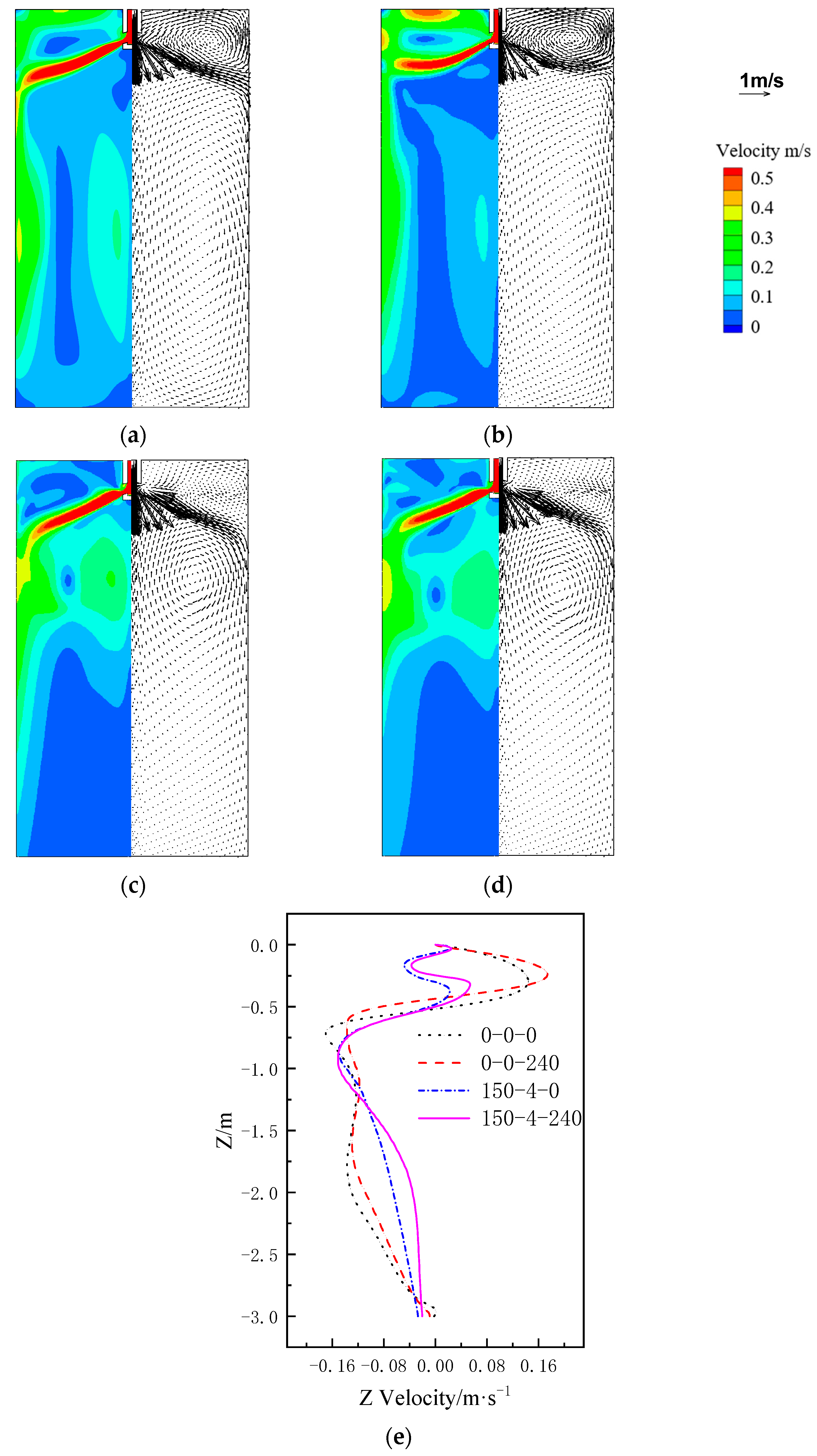
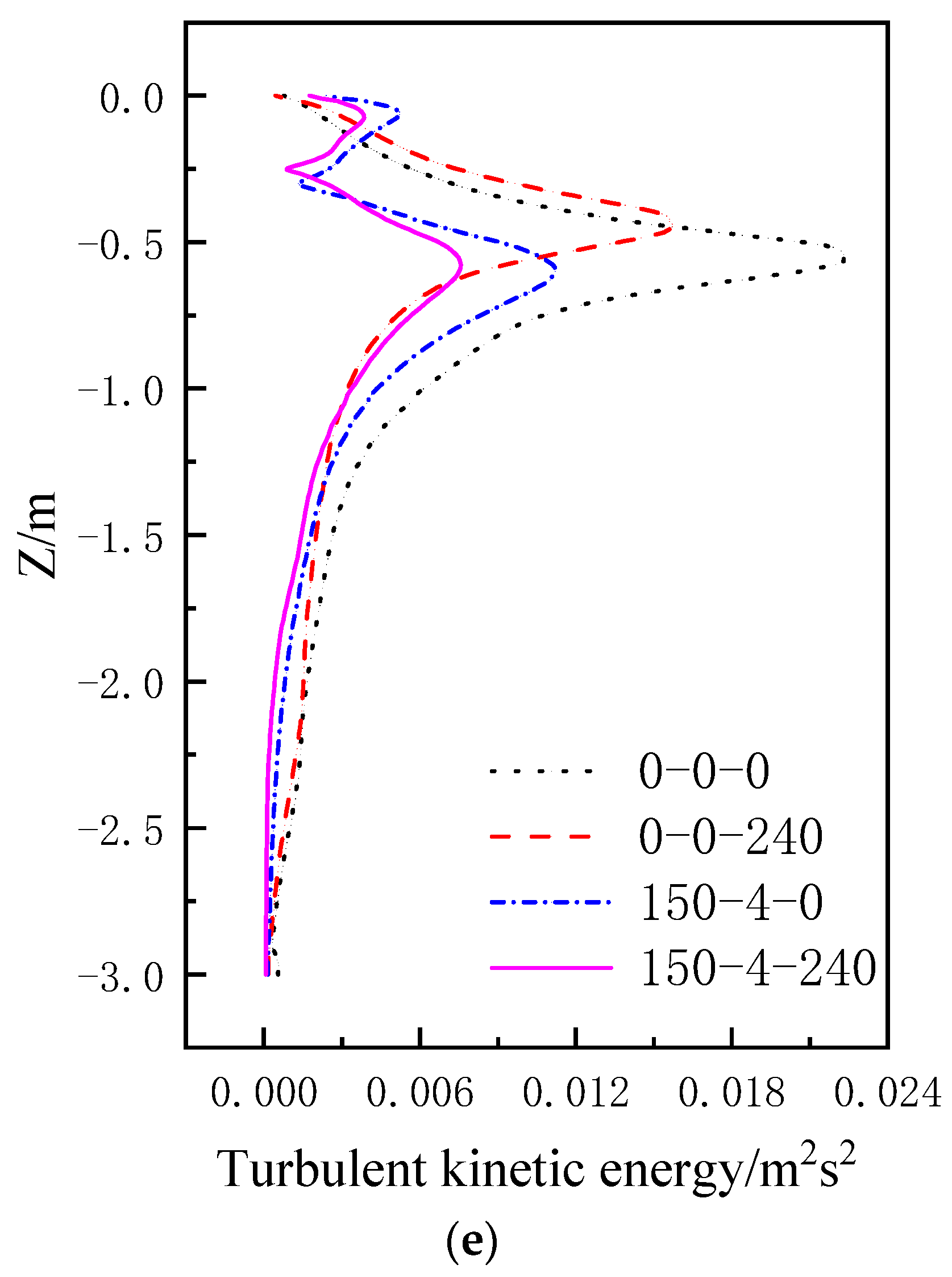
3.2. Flow Field Simulation

Figure 6 shows the velocity contour and the vector distribution of the flow in the wide central section of the mold under different electromagnetic parameters (a) without the magnetic field, (b) with EMBr only, (c) with EMS only, and (d) with composite magnetic cases, respectively. In Figure 6a, due to the absence of a magnetic field, the velocity of upward flow and downward flow is very fast, and the impinging depth of jet flow is deep. The flow field is similar to the results in the reference [1]. In Figure 6b, due to the Lorentz force generated with the EMBr, the jet flow has an obvious rise, the upward flow is enhanced, the downward flow is slightly weakened, and the impinging depth of the jet flow is also reduced. This is also similar to the results in the reference [14]. Figure 6c shows the flow field under the effect of the EMS only. The rotating electromagnetic force also affects the behavior of the jet flow, which significantly reduces the impinging depth of the jet flow. This is also similar to the results in the reference [19]. Figure 6d shows the flow field under the composite magnetic field. The impinging depth of the jet flow is further reduced than that in Figure 6b, c. The velocity distribution in the Z-direction at the vertical centerline of a narrow face is shown in Figure 6e. There is a significant difference in the upward flow between with and without EMS. Comparing that without magnetic field and in EMBr only, the downward flow in only EMS and in the composite magnetic field is obviously weakened, the impinging depth of jet flow is lower, and the effect of the composite magnetic field is the largest. The maximum absolute value overall of the Z-direction velocity of the upward flow is maximumly decreased by 56%, while the maximum absolute value overall of the Z-direction velocity of the downward flow is maximumly decreased by 12%; the impinging depth of the jet flow of the molten steel decreases by about 20 mm.

Figure 7 shows the contour and vector distribution of velocity at 10 mm cross section below the meniscus in different conditions. In Figure 7a, when there is no magnetic field, the velocity distribution at the meniscus converges from the narrow side to the SEN. Because of the instability of turbulence, the distribution of the left and the right flow fields is not completely symmetrical. The surface velocity at one side of the SEN is slightly higher than that at the other side, making it possible to cross the center line and merge with the surface flow at the other side to generate circulation. When the circulation velocity exceeds the critical value, vortices may form. In Figure 7b, due to the lifting effect of the EMBr, the downward flow on the jet flow is enhanced, and the velocity at the meniscus is increased. The velocity distribution mode is similar to that without a magnetic field. In Figure 7c, the rotating electromagnetic force of EMS makes the meniscus rotate clockwise, which has a good control effect on the velocity of the meniscus. In Figure 7d, in the composite magnetic field and under the effect of the EMBr, the jet flow has an obvious rise. The upward flow is enhanced and that weakens the stirring effect of the EMS at the meniscus, but it still forms the weaker clockwise stirring effect than that with EMS only.

Figure 8 shows the contour of turbulent kinetic energy at the 10 mm section below the meniscus in different conditions. In Figure 8a, the intensity of turbulent kinetic energy at the meniscus is weak because there is no rotating electromagnetic force of EMS. In Figure 8b, compared with the case of 0-0-0 like in Figure 8a, the intensity of the turbulent kinetic energy increases slightly, as a result of the increase in the velocity of the molten steel at the meniscus. In Figure 8c, the rotating electromagnetic force produced with the EMS makes the turbulent kinetic energy intensity of the meniscus increase significantly, but the turbulent kinetic energy at the corner is excessively large. In Figure 8d, the EMBr enhances the upward flow, which weakens the EMS at the meniscus, and in general, the turbulent kinetic energy at the meniscus is slightly weaker than that of EMS only. And especially, the turbulent kinetic energy at the corner is much lower than that in Figure 8c.

Figure 9 is the velocity vector and the turbulent kinetic energy contour of the vertical section at a distance of 5 mm from the narrow face. In Figure 9a, because there is no external magnetic field to control the flow of molten steel, the jet flow velocity is very large, resulting in a large impact strength on the narrow face. In Figure 9b, the EMBr makes the jet flow rise upward, and the Lorentz force produced in the opposite direction of the jet flow reduces the flow velocity of the jet flow and the impact strength on the narrow face.

In Figure 9c, the jet flow does not impact the narrow plane vertically. The impact strength on the narrow plane is weakened because of the rotating electromagnetic force generated using the EMS which causes rotation at the meniscus. Due to the inertial effect of the fluid, rotation affects the movement behavior of the jet flow, making the jet flow deflect (similar to the effect of electromagnetic swirling on the SEN) [27]. In Figure 9d, under the joint action of EMS and EMBr, the impact strength of the jet flow on the narrow face is further weakened. The turbulent kinetic energy at the center line of the narrow face is shown in Figure 9e. Under the four different conditions—without magnetic, EMBr only, EMS only, and composite magnetic—the maximum turbulent kinetic energy of the jet flow impact on the narrow face is 0.0224 m² s², 0.0158 m² s², 0.011 m² s², and 0.0075 m² s², respectively, which is in a descending order.

3.3. Experimental Verification

The results of the numerical simulation are verified using model experiments of the low melting point alloy Pb-Sn-Bi under composite magnetic field. The mass content is 30% of Pb, 20% of Sn, and 50% of Bi. The physical properties of molten Pb-Sn-Bi alloys are similar to those of molten steel [28]. It is feasible to simulate molten steel flow under an electromagnetic field using this alloy. In the model experiment, the mold size was 375 mm × 63 mm × 750 mm. The alloy temperature was 180 °C, the conductivity was 1.11 s/m, the density was 9500 kg/m³, the relative permeability was 1, and the casting speed was 0.45 m/min, respectively. A CT3-A pointer type Tesla meter and an ultrasonic Doppler velocimeter (UDV) (Signal processing S.A) were used to measure the magnetic field and fluid velocity in the experiment, respectively. The CT3-A pointer type Tesla meter resolution could reach 0.02 mT, with an application frequency range of 0–600 Hz. The diameter and the transmission frequency of the UDV was 12 mm and 2 MHz, respectively, and the resolution was 2250 ns. Such kinds of measurement methods were well used by us [29,30]. To simulate experiments of the slab continuous casting process of steel under the composite magnetic field, we used 350 kg of molten alloy, as shown in Figure 10a. The level of molten alloy was maintained at the same level during the casting process.

The magnetic induction intensity at the center of electromagnetic stirring on the mold wall was measured under a composite magnetic field, and it was compared with the numerical simulation results under the same experimental composite magnetic field setup and current parameters, as shown in Figure 10b. The trend of the magnetic induction intensity change at the same location is basically similar. The average error between the experimental and the numerical result is about 4.1%, proving the good accuracy of the composite magnetic field numerical simulation method used in this paper. The velocity was measured with the probe at 20 mm below the meniscus and 1/4 of the narrow face, and the measured velocity in the extension line of the probe is compared with the numerical simulation results of the flow field under the same parameters of the composite magnetic field, as shown in Figure 10c. The trend of the velocity change in the experiment is consistent with the numerical simulation results, showing a trend of first increasing and then decreasing. The average error between the numerical calculation results and the overall measured steel flow rate is about 3.2%, proving the feasibility of the flow field simulation method under composite magnetic fields.

4. Conclusions

In this paper, a three-dimensional numerical simulation model of the composite magnetic field of the EMS and a ruler-type EMBr in the slab mold and a model of the flow field under the composite magnetic field was established and verified. The magnetic field under the composite magnetic field was calculated, and the results were introduced into the numerical calculation of the flow field. These results were compared with those under different magnetic field conditions. The following conclusions were obtained:

The magnetic induction intensity generated using the EMS will not interfere with that in the EMBr area; the component of the magnetic induction intensity generated with the EMBr in the EMS area is almost in the same order with that using EMS, but the electromagnetic force with EMBr here is about 1/30–1/300 of that using EMS, which can be ignored.

Under the ruler type of the composite magnetic field, the maximum velocities of the upward flow and the downward flow in the mold decreased maximumly by 56% and 12%, respectively. The impact depth of the jet flow of molten steel on the narrow surface rose by about 20 mm. The upward flow moved down slightly as a whole, and the molten steel on the meniscus formed a clockwise circulation flow. The velocity distribution and the turbulent kinetic energy near the meniscus was generally more uniformed.

Under the ruler type of the composite magnetic field, the EMBr and the EMS can play their respective roles well under certain conditions, the impact of the jet flow on the narrow face is reduced, and the stirring beneath the meniscus is intensified.

References

1. Cho, S.M.; Thomas, B.G. Electromagnetic Forces in Continuous Casting of Steel Slabs. Metals 2019, 9, 471. [Google Scholar] [CrossRef] [Green Version]
2. Wang, C.; Liu, Z.; Li, B. Combined Effects of EMBr and SEMS on Melt Flow and Solidification in a Thin Slab Continuous Caster. Metals 2021, 11, 948. [Google Scholar] [CrossRef]
3. Liu, G.; Lu, H.; Li, B.; Ji, C.; Zhang, J.; Liu, Q.; Lei, Z. Influence of M-EMS on Fluid Flow and Initial Solidification in Slab Continuous Casting. Materials 2021, 14, 3681. [Google Scholar] [CrossRef]
4. Li, Z.; Zhang, L.; Bao, Y.; Ma, D.; Wang, E. Influence of the Vertical Pole Parameters on Molten Steel Flow and Meniscus Behavior in a FAC-EMBr Controlled Mold. Metall. Mater. Trans. B 2022, 53, 938–953. [Google Scholar] [CrossRef]
5. Bao, Y.; Li, Z.; Zhang, L.; Wu, J.; Ma, D.; Jia, F. Asymmetric Flow Control in a Slab Mold through a New Type of Electromagnetic Field Arrangement. Processes 2021, 9, 1988. [Google Scholar] [CrossRef]
6. Guo, Y.; Yang, J.; Liu, Y.; He, W.; Zhao, C.; Liu, Y. Numerical Simulation of Flow Field, Bubble Distribution and Solidified Shell in Slab Mold under Different EMBr Conditions Assisted with High-Temperature Quantitative Velocity Measurement. Metals 2022, 12, 1050. [Google Scholar] [CrossRef]
7. Jiang, D.; Zhu, M.; Zhang, L. Numerical Simulation of Solidification Behavior and Solute Transport in Slab Continuous Casting with S-EMS. Metals 2019, 9, 452. [Google Scholar] [CrossRef] [Green Version]
8. Liu, Z.; Li, B. Transient motion of inclusion cluster in vertical-bending continuous casting caster considering heat transfer and solidification. Powder Technol. 2016, 287, 315–329. [Google Scholar] [CrossRef]
9. Li, B.; Lu, H.; Zhong, Y.; Ren, Z.; Lei, Z. Influence of EMS on Asymmetric Flow with Different SEN Clogging Rates in a Slab Continuous Casting Mold. Metals 2019, 9, 1288. [Google Scholar] [CrossRef] [Green Version]
10. Wang, W.; Chen, S.; Lei, H.; Zhang, H.; Xiong, H.; Jiang, M. Inclusion Behavior in a Curved Bloom Continuous Caster with Mold Electromagnetic Stirring. Metals 2020, 10, 1580. [Google Scholar] [CrossRef]
11. Liu, Z.; Li, L.; Qi, F.; Li, B.; Jiang, M.; Tsukihashi, F. Population balance modeling of polydispersed bubbly flow in continuous-casting using multiple-size-group approach. Metall. Mater. Trans. B 2015, 46, 406–420. [Google Scholar] [CrossRef]
12. Wang, Q.; Zhang, L. Influence of FC-mold on the full solidification of continuous casting slab. JOM 2016, 68, 2170–2179. [Google Scholar] [CrossRef]
13. Zhang, L.; Xu, C.; Zhang, J.; Wang, T.; Li, J.; Li, S. The simulation and optimization of an electromagnetic field in a vertical continuous casting mold for a large bloom. Metals 2020, 10, 516. [Google Scholar] [CrossRef] [Green Version]
14. Schurmann, D.; Glavinić, I.; Willers, B.; Timmel, K.; Eckert, S. Impact of the electromagnetic brake position on the flow structure in a slab continuous casting mold: An experimental parameter study. Metall. Mater. Trans. B 2020, 51, 61–78. [Google Scholar] [CrossRef]
15. Wang, Y.; Zhang, L. Fluid flow-related transport phenomena in steel slab continuous casting strands under electromagnetic brake. Metall. Mater. Trans. B 2011, 42, 1319–1351. [Google Scholar] [CrossRef]
16. Li, Z.; Zhang, L.; Ma, D.; Wang, E. Numerical Simulation on Flow Characteristic of Molten Steel in the Mold with Freestanding Adjustable Combination Electromagnetic Brake. Metall. Mater. Trans. B 2020, 51, 2609–2627. [Google Scholar] [CrossRef]
17. Vakhrushev, A.; Kharicha, A.; Liu, Z.; Wu, M.; Ludwig, A.; Nitzl, G.; Tang, Y.; Hackl, G.; Watzinger, J. Electric Current Distribution During Electromagnetic Braking in Continuous Casting. Metall. Mater. Trans. B 2020, 51, 2811–2828. [Google Scholar] [CrossRef]
18. Fang, Q.; Ni, H.; Zhang, H.; Wang, B.; Lv, Z. The effects of a submerged entry nozzle on flow and initial solidification in a continuous casting bloom mold with electromagnetic stirring. Metals 2017, 7, 146. [Google Scholar] [CrossRef] [Green Version]
19. Liu, Z.; Li, B.; Wu, M.; Xu, G.; Ruan, X.; Ludwig, A. An experimental benchmark of non-metallic inclusion distribution inside a heavy continuous-casting slab. Metall. Mater. Trans. A 2019, 50, 1370–1379. [Google Scholar] [CrossRef]
20. Yin, Y.; Zhang, J.; Lei, S.; Dong, Q. Numerical Study on the Capture of Large Inclusion in Slab Continuous Casting with the Effect of In-mold Electromagnetic Stirring. ISIJ Int. 2017, 57, 2165–2174. [Google Scholar] [CrossRef] [Green Version]
21. Cho, S.M.; Thomas, B.G.; Kim, S.H. Effect of nozzle port angle on transient flow and surface slag behavior during continuous steel-slab casting. Metall. Mater. Trans. B 2019, 50, 52–76. [Google Scholar] [CrossRef]
22. Zhong, Y.T.; Pan, H.Y.; Jacobson, N.; Sedén, M. Development trends of mold flow control in slab casting. Baosteel Technol. 2016, 5, 53–57. [Google Scholar] [CrossRef]
23. Sun, X.; Li, B.; Lu, H.; Zhong, Y.; Ren, Z.; Lei, Z. Steel/Slag Interface Behavior under Multifunction Electromagnetic Driving in a Continuous Casting Slab Mold. Metals 2019, 9, 983. [Google Scholar] [CrossRef] [Green Version]
24. Han, S.-W.; Cho, H.-J.; Jin, S.-Y.; Sedén, M.; Lee, I.-B.; Sohn, I. Effects of Simultaneous Static and Traveling Magnetic Fields on the Molten Steel Flow in a Continuous Casting Mold. Metall. Mater. Trans. B 2018, 49, 2757–2769. [Google Scholar] [CrossRef]
25. Yang, Y.; Jönsson, P.G.; Ersson, M.; Su, Z.; He, J.; Nakajima, K. The influence of swirl flow on the flow field, temperature field and inclusion behavior when using a half type electromagnetic swirl flow generator in a submerged entry and mold. Steel Res. Int. 2015, 86, 1312–1327. [Google Scholar] [CrossRef]
26. Schneiders, R. A grid-based algorithm for the generation of hexahedral element meshes. Eng. Comput. 1996, 12, 168–177. [Google Scholar] [CrossRef]
27. Garcia-hernandez, S.; Morales, R.D.; Torres-Alonso, E. Effects of EMBr position, mould curvature and slide gate on fluid flow of steel in slab mould. Ironmak. Steelmak. 2010, 37, 360–368. [Google Scholar] [CrossRef]
28. Chen, Z.; Wang, E.; Zhang, X.; Wang, Y.; Zhu, M.; He, J. Study on the behavior of bubbles in a continuous casting mold with Ar injection and traveling magnetic flied. Acta Metall. Sin. 2012, 48, 951–956. [Google Scholar] [CrossRef]
29. Chen, J.; Su, Z.; Li, D.; Wang, Q.; He, J. Flow Behavior in the Slab Mold under Optimized Swirling Technology in Submerged Entry Nozzle. ISIJ Int. 2018, 58, 1242–1249. [Google Scholar] [CrossRef] [Green Version]
30. Li, D.; Su, Z.; Chen, J.; Wang, Q.; Yang, Y.; Nakajima, K.; Marukawa, K.; He, J. Effects of Electromagnetic Swirling Flow in Submerged Entry Nozzle on Square Billet Continuous Casting of Steel Process. ISIJ Int. 2013, 53, 1187–1194. [Google Scholar] [CrossRef] [Green Version]
Figure 1. Mesh of the computational domain for (a) magnetic field; (b) flow field.
Metals 13 01237 g001
Figure 2. Structure of composite magnetic field. (a) Wide face side view; (b) narrow face side view.
Metals 13 01237 g002
Figure 3. (a) Contour plot of the magnetic flux density in the mold under EMS only; distribution of the magnetic flux intensity at (b) ab and cd lines and (c) ef and gh lines.
Metals 13 01237 g003
Figure 4. (a) The vector and (b) the magnitude of time average electromagnetic force at the section 50 mm below the meniscus of the mold.
Metals 13 01237 g004aMetals 13 01237 g004b
Figure 5. (a) Contour plot of the magnetic flux density in the mold under EMBr only; distribution of magnetic flux intensity at different positions of wide central section of mold (Time = 0). (b) ab and cd line; (c) ef and gh line.
Metals 13 01237 g005aMetals 13 01237 g005b
Figure 6. Velocity contour of wide central section of mold (a) 0-0-0; (b) 0-0-240; (c) 150-4-0; and (d) 150-4-240. (e) Velocity distribution in Z-direction at the vertical centerline of the near narrow face.
Metals 13 01237 g006
Figure 7. Contour and vector of velocity at 10 mm section below meniscus. (a) 0-0-0; (b) 0-0-240; (c) 150-4-0; (d) 150-4-240.
Metals 13 01237 g007
Figure 8. Contour of turbulent kinetic energy at 10 mm section below meniscus. (a) 0-0-0; (b) 0-0-240; (c) 150-4-0; (d) 150-4-240.
Metals 13 01237 g008
Figure 9. Velocity vector and turbulent kinetic energy contour at 5 mm on narrow face. (a) 0-0-0; (b) 0-0-240; (c) 150-4-0; (d) 150-4-240; (e) turbulent kinetic energy at the center line of narrow plane.
Metals 13 01237 g009aMetals 13 01237 g009b
Figure 10. (a) Experimental device; (b) verification of magnetic field numerical simulation results and experimental measurements; (c) flow velocity’s contrast on mold of composite magnetic field between experiment and simulation.
Metals 13 01237 g010