Article

Modeling Microstructure Development upon Continuous Cooling of 42CrMo4 Steel Grade for Large-Size Components

by
Sergio Fernandez-Sanchez
1,2,
Amaia Iza-Mendia
1,2 and
Denis Jorge-Badiola
1,2,*
1
Ceit-Member of Basque Research & Technology Alliance (BRTA), 20018 Donostia-San Sebastián, Gipuzkoa, Spain
2
Mechanical Engineering and Materials Department, Tecnun-Universidad de Navarra, 20018 Donostia-San Sebastián, Gipuzkoa, Spain
*
Author to whom correspondence should be addressed.
Metals 2024, 14(10), 1096; https://doi.org/10.3390/met14101096
Submission received: 11 August 2024 / Revised: 19 September 2024 / Accepted: 21 September 2024 / Published: 24 September 2024
(This article belongs to the Special Issue Advances in Phase Transformation Behavior of Steels)

Abstract

:
42CrMo4-type steel grades are widely used in a great variety of components that require ad hoc mechanical properties. However, due to the dimensions of large components and the previous thermomechanical treatments, the presence of heterogeneities in the chemical compositions are expected to impact those mechanical properties. In the present work, a detailed analysis of phase transformation behavior upon cooling was carried out through a dilatometry test on samples of 42CrMo4 belonging to a component that has a non-homogeneous chemical distribution. The analysis of the dilatation signals and the quantitative metallography shows a rather complex behavior depending on the cooling rate as well as on the region of observation. Two different phase transformation models based on Li’s approach were applied to the present composition to determine the CCT curve as well as the fraction of the microconstituents. An extensive discussion was carried out on some aspects about Kirkaldy-based approaches that need to be improved so as to attain more reliable quantitative results when modeling phase transformations in heterogenous systems.

1. Introduction

42CrMo4 (AISI 4140) steel grade is applied in a wide variety of applications in sectors such as automotive [1], oil and gas [2] and wind energy [3] due to its appealing mechanical properties and a relatively low amount of various alloying elements. In that regard, a large amount of literature on this steel grade can be found that embraces not only the mechanical aspects [1,4], but also corrosive behavior [5,6] and microstructure development [7,8].
The use of this steel grade in large parts has become of particular interest in the last years, as discussed elsewhere [9]. These large parts, after thermomechanical treatments like forging [7], are heat-treated to achieve the targeted mechanical properties. For instance, quenching and tempering is usually applied so as to accomplish a tempered martensite structure [9,10]. However, due to the size of the parts, the microstructural evolution, as inner regions are analyzed, presents a higher degree of complexity. Moreover, such large parts, like large flanges or shafts fabricated from ingots, exhibit a complex chemical pattern leading to heterogeneity, which stems from the solidification, and cannot be homogenized all through the thermomechanical treatment [11]. Depending on the scale, this kind of segregation can be categorized as macrosegregation, microsegregation and mesosegregation, the latter usually being arranged in the form of bands [12,13]. Another source of heterogeneity may arise from the changing austenite grain size along the material, which is often connected to the chemical heterogeneity [14].
Looking at numerical modeling of the phase transformation on the continuous cooling of steels, there are different approaches that can be organized in terms of nature, computing time and predictive capabilities [15]. The physics-based approaches for phase transformation modeling, which rely on the physical phenomena—nucleation/growth, for instance [16,17,18]—and may account for the real initial microstructure [19], excel in predictions with regard to other models. However, their complexity, expectedly, demands higher computational cost and they are often of limited applicability, as many of the parameters are not readily suitable for multicomponent and multiphase alloys [20], unless thermodynamic and kinetics simulations are used [21]. With the advent of the data-driven models, both factors can be optimized [22], but a significant amount of data are needed, and these are not always available. Conversely, phenomenological models, JMAK or Kirkaldy types, which are linked to some physical and process parameters, are extensively applied due to the easiness of their implementation, low computational cost and the need for a relatively reduced number of experiments to fit the models. In this line, Li et al.’s variant of the former Kirkaldy–Venogupalan formulation [23] can be found open-coded by A.S. Nishikawa in [24], which gives the possibility to predict the microstructural evolution upon cooling. Lately, Collins et al. [25] have proposed another variant also based on Li’s approach, but with a significant number of new features related to the carbon partitioning and bainite transformation, amongst others. These two works, open-access coded [24,26], facilitate the possibility to predict rapidly the phase transformation behavior upon continuous cooling (CCT: continuous cooling transformation) in a simple way. Either case can be adapted to the problem of chemical heterogeneity observed in large parts. On the other hand, commercial models, such as JMatPro, Thermo-Calc, etc., are also available for predicting the microstructural evolution upon cooling. However, the degree of goodness in the prediction of the CCT and the final microconstituents fractions need to be thoroughly assessed and validated in real industrial steels, in which heterogeneities play a significant role.
Some prior works on the microstructure evolution in 42CrMo4 steel during continuous cooling can be found in the literature [4,27]. However, to the authors’ knowledge, a specific study that accounts for the heterogeneity from the quantitative and modeling perspectives is not reported in the literature. In the present work, the main objective is to perform a thorough analysis of the microstructural development of a 42CrMo4 steel, machined from a large industrial part, upon continuous cooling, considering both the experimental observations and insights from the modeling The large part inherits the microstructure and chemical heterogeneities from both microstructure and chemical perspectives. The experimental activities have a double aim. On the one hand, the detailed understanding of the microstructural development and cooling cycle relationship and, on the other hand, the phase quantification for the assessment and calibration of some available phase transformation models at Ceit. Moreover, the results of the models are compared with the experimental data. The need for improvements in terms of proper optimization of the parameters in the models and the introduction of the heterogeneities in the prediction of the experimental data are tackled for this steel grade.

2. Experimental Section

The chemical composition of the steel grade used in this work is gathered in Table 1, which corresponds to a 42CrMo4-type steel.
The material was provided after an industrial process, which consists in a solution heat treatment above 1200 °C for more than typically 4 h of a large ingot, upsetting, piercing, hot forming and final quenching. Before designing the thermal cycles, the Thermo-Calc program (Thermo-Calc Software v2023.1.108587-453, AB Råsundavägen, Solna, Sweden) with the TCFe10 database was run with the composition in Table 1; see Figure 1. The phase diagram shows that except for the Nb/Ti carbonitrides, the rest of the carbides, mainly cementite, are fully dissolved at temperatures above 760 °C.
The thermal cycles were performed in a Bähr DIL805D deformation dilatometer (TA Instruments, Hüllhorst, Germany) on solid cylinders of 10 mm length and 4 mm diameter. The applied thermal cycles consist in a two-stage heating segment: 10 °C/s up to 700 °C followed by 0.5 °C/s up to three austenization temperatures T a u s = 850 °C, 1050 °C and 1100 °C, respectively, followed by a holding stage for 900 s at those temperatures and a final cooling stage at rates between −0.025 °C/s and −50 °C/s down to room temperature. The range of cooling rates was chosen based on thermal profiles determined by FE (Finite Elements) simulations at different radial positions of a steel cylinder of 1000 mm diameter quenched in water; see Figure 2.
All the metallographic observations were performed on the midsection of the cylindrical dilatometric samples. The samples were mechanically polished down to 1 µm. To ensure the avoidance of temperature gradients and any decarburization close to the surfaces of the samples, the microstructural characterization was performed on the central region of the midsection. The microstructures were characterized with different techniques:
  • Optical microscopy (OM, LEICA DMI5000 M, Leica Microsystems, Wetzlar, Germany) for general observations and metallographic quantifications;
  • Field-emission gun scanning electron microscopy (Zeiss Sigma 500, SEM, Carl Zeiss AG, Oberkochen, Germany) for detailed imaging of some microstructure constituents;
  • Microchemical analysis by EDS energy dispersive spectroscopy (X-Max® 50 EDS analyzer, Oxford Instruments, Abingdon, UK) fully controlled by the latest AZtec software 3.0 SP2 (Oxford Instruments, Abingdon, UK). The AZtec program allows creating quantitative results through the application of the TruLine algorithm that deconvolutes the peaks in case of overlapping and removes the background automatically.
The previous austenite was analyzed in optical images after picric acid etching. The grain size distribution as well as the mean grain size were determined by tracing the grain boundary structure and using the software Leica Application Suite LAS V4.5 LEICA (Leica Microsystems, Wetzlar, Germany) for identifying and measuring the grain size.
The phase fraction quantification was performed on optical micrographs after etching in 2% Nital and applying the point-counting method. As shown in Figure 3a, the microstructure can be highly heterogeneous for its quantification when large areas such as the whole length of the dilatometer sample are analyzed.
With the aim of measuring the fraction of the various microconstituents, a strategy based on two sets of micrographs, one at low magnifications and one at higher magnifications, was undertaken. Dark and bright regions are readily distinguishable at low magnifications, Figure 3a. Accordingly, it is possible to measure the fractions corresponding to each region. High magnification micrographs allow segmenting each region and identifying each microconstituent, Figure 3b. Again, the point-counting method is applied on each region to quantify the phase fractions. Finally, the total fraction of each microconstituent is defined as the sum of the ponded fraction of the microconstituent by the area fraction of each region, Equation (1).
F i = F B F i B + F D F i D
where F i is the fraction of the i -microconstituent, F B and F D are the bright and dark region fractions and F i B and F i D are the fractions of the i -microconstituent considering only the bright and dark regions. From this point on, F, P, B and M will stand for ferrite, pearlite, bainite and martensite, respectively.
Hardness measurements (Vickers 1 kg) were performed in a QNESS Q30A+ (microhardness tester, QATM, Golling an der Salzach, Austria) on a set of 18 points that were spatially arranged in a random manner.
Regarding modeling parts, two approaches based on Li’s approach [24,26] for the CCT modeling were undertaken by applying open-source software. Further details of the approaches are given in the discussion section.

3. Results

The main results of this study are summarized in the next sections looking at five main points:
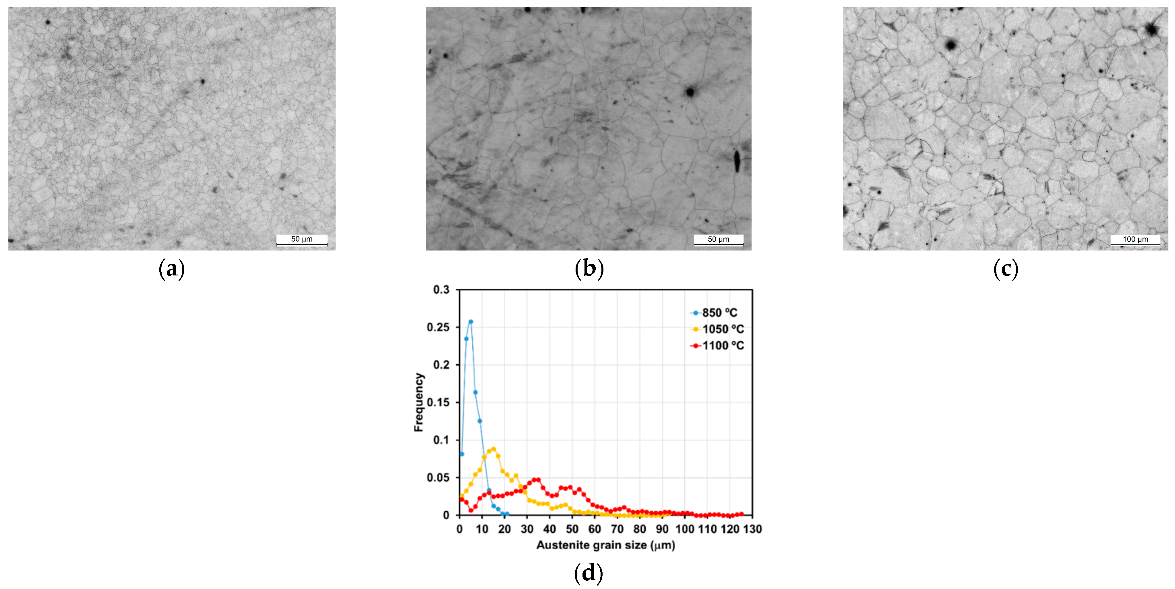
  • Austenite grain size evolution with austenization temperature;
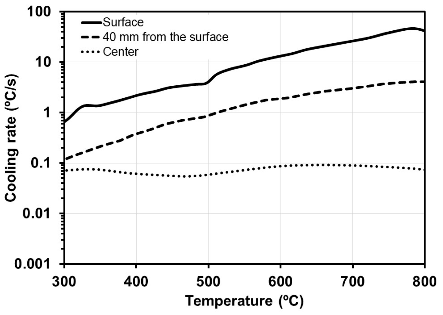
  • Determination of the CCT curves for the three austenization temperatures;
  • Hardness evolution with cooling rate;
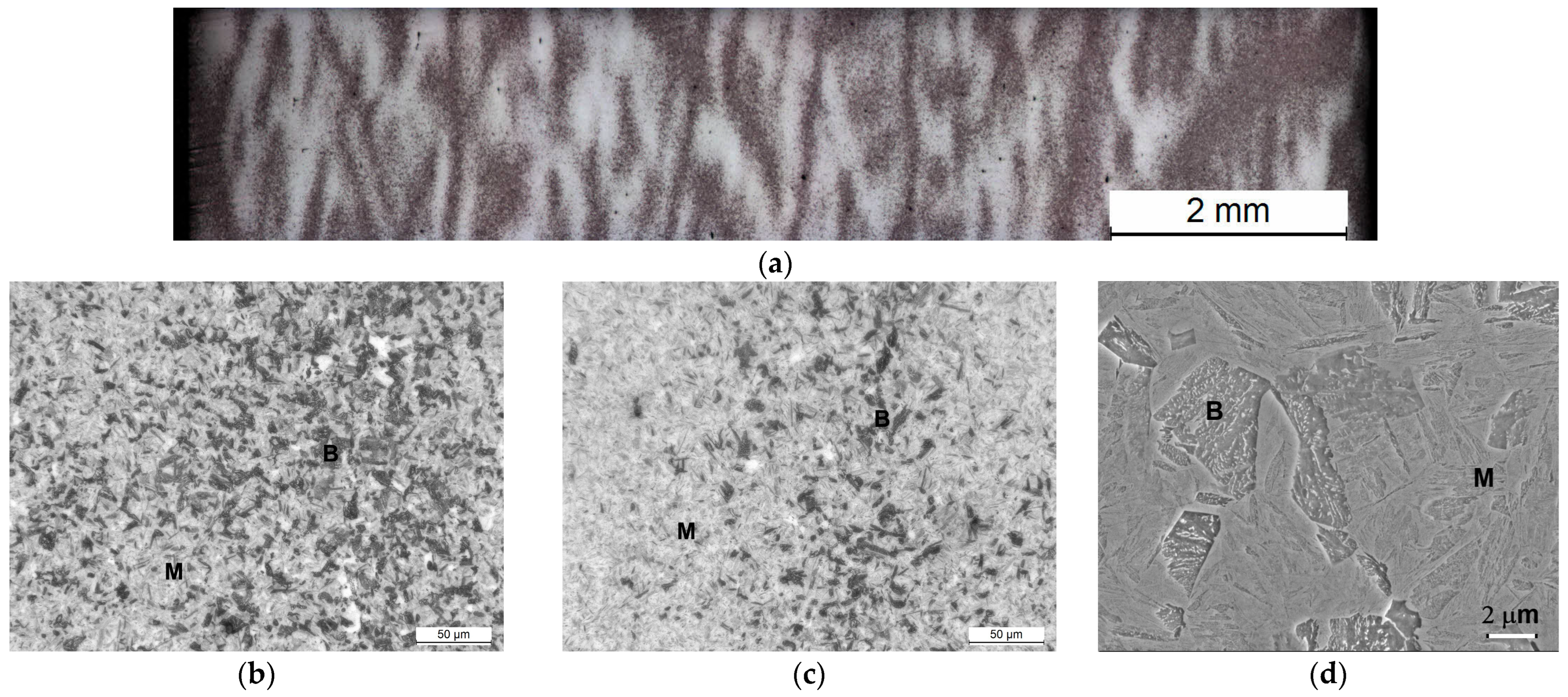
  • Microstructural evolution with the cooling rate;
  • Application of the open-source codes and commercial simulators to the nominal composition, Table 1, for CCT determination.

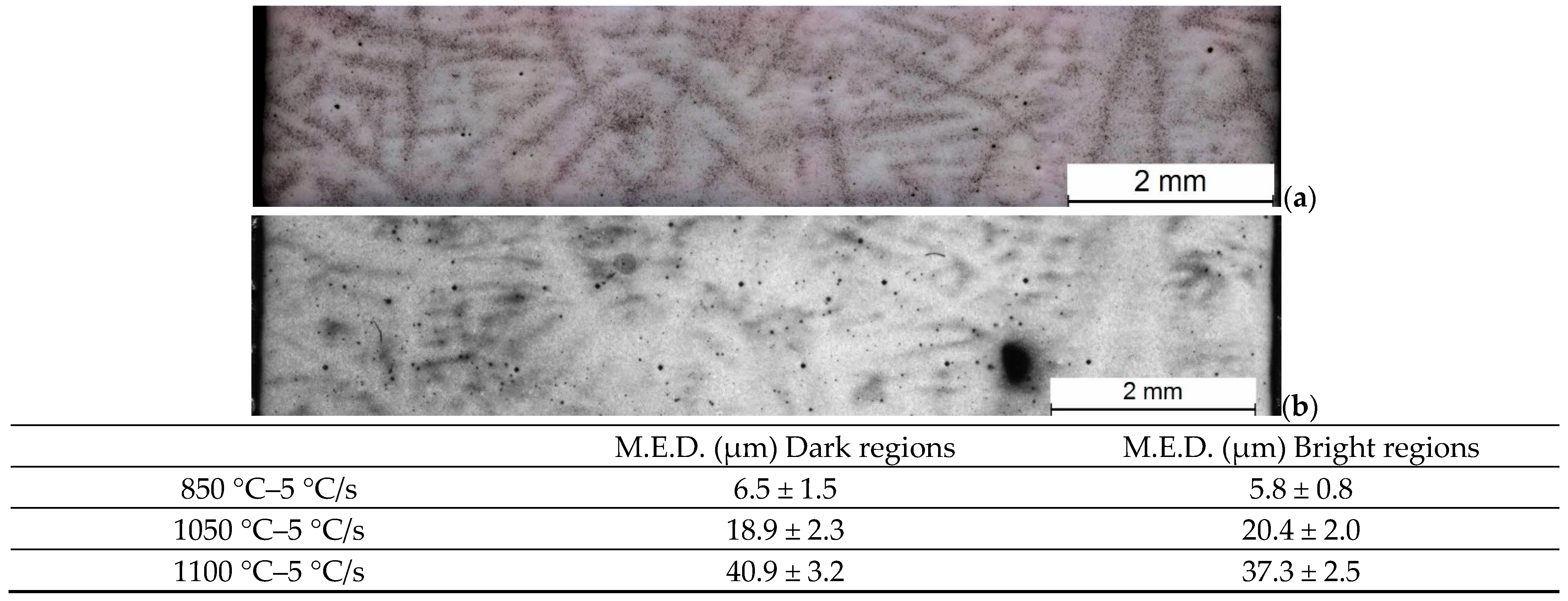
3.1. Austenite Grain Size
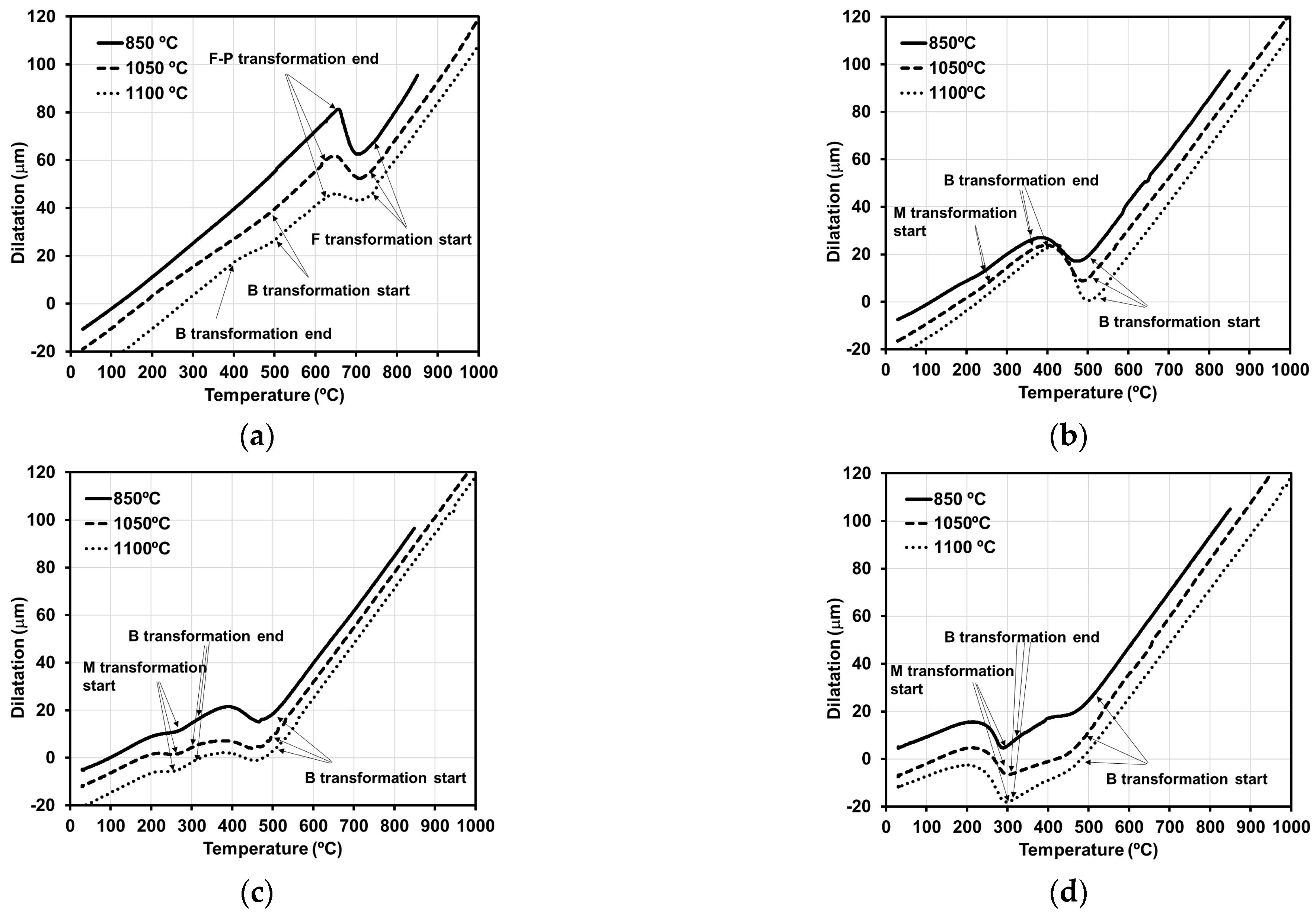
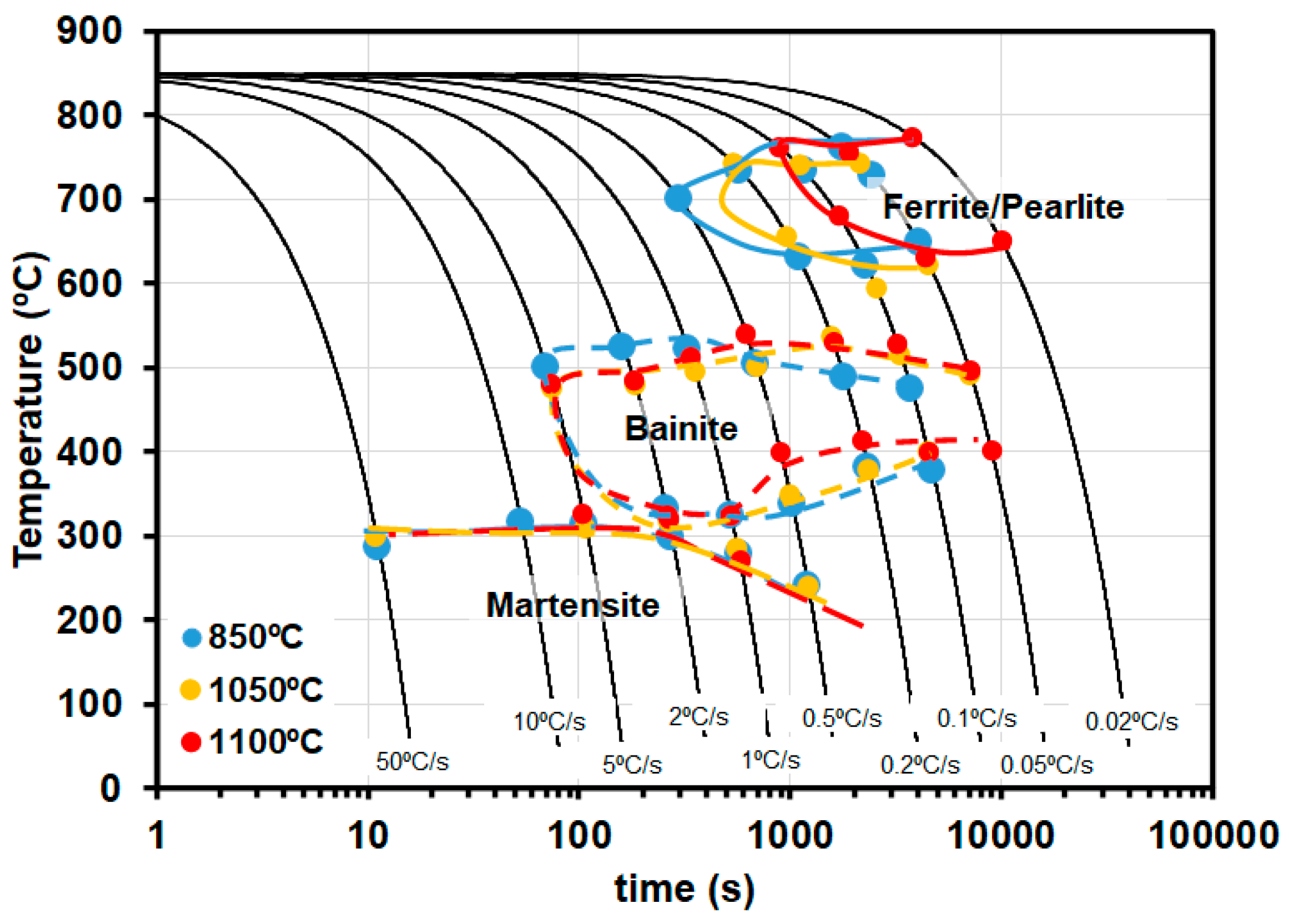
The austenite grain size structures after the three holding temperatures are shown in Figure 4a–c. The achieved grain sizes were about 6, 20 and 38 µm for holding temperatures of 850 °C, 1050 °C and 1100 °C, respectively. The range of grain sizes is large enough for modeling purposes. Moreover, the grain size distribution was determined for each condition, Figure 4d. It is to be mentioned that, in general, the distributions seem to be homogeneous except for a few grains for the highest austenitizing temperature of 1100 °C, which appears to be related to the onset of the abnormal grain growth.
Additionally, the spatial distribution of the austenite grain size was analyzed, trying to discern whether it is correlated to the chemical pattern detected in micrographs such as the one in Figure 5a. Samples corresponding to cooling rates of 5 °C/s were gently (re)polished and etched with the picric acid, Figure 5b.
The results in Figure 5 prove that the chemical pattern is not correlated to likely changes in the austenite grain size. Indeed, the grain size is spatially homogeneous and the grain size effect on the phase transformation can be dismissed in the present work.

3.2. CCT Curves

Several dilatation curves with temperature are shown in Figure 6. As can be seen, the different phase transformation curves for the same cooling rate differ for each austenitizing temperature. The onset and finish of the different phase transformations was determined through the analysis of the dilatation curves. In particular, the phase transformation occurs when the slope of the curves changes significantly.
The CCT (Continuous Cooling Transformation) curves were determined for three different mean austenite grain sizes of 6, 20 and 38 μm, Figure 7.
The effect of the austenitizing temperature on the CCT curve can be described as follows. The ferritic-pearlitic field is clearly retarded to lower cooling rates at T a u s above 1050 °C. In fact, there is no signal of ferrite-pearlite transformation for 1100 °C and a cooling rate of 0.2 °C/s. The range of cooling rates in which bainite transformation takes place moves to the left, has shorter times, and disappears at more sluggish rates when the lowest T a u s , 850 °C, is applied. Interestingly, there is a range of cooling rates, from 0.2 to 0.5 °C/s, for the highest austenization temperature, 1100 °C, in which only bainite seems to be the main microstructure constituent. For cooling rates faster than 5 °C/s, the microstructure is fully martensite irrespective of the austenization temperature.

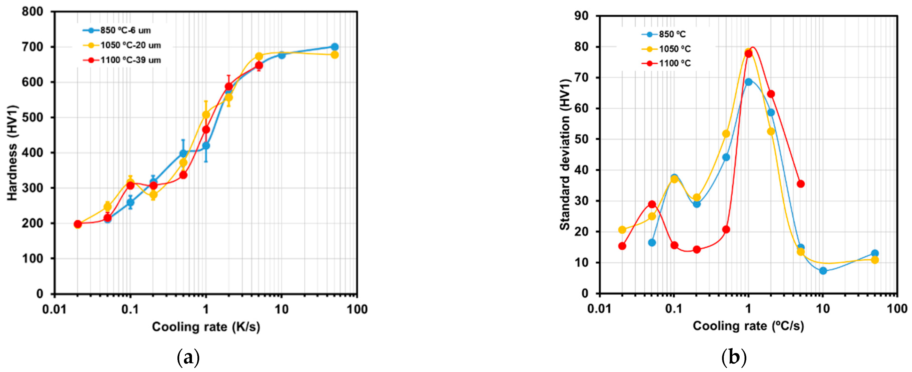
3.3. Hardness Evolution

The evolution of hardness with the cooling rate and austenization temperature is shown in Figure 8. The change in hardness can be roughly divided into three cooling rate regions: below 0.2 °C/s, above 2 °C/s and in-between these two cooling rates. The increase in hardness between 0.02 °C/s and 0.2 °C/s and between 2 °C/s and 20 °C/s is about 100 HV1, whereas the steepest increase is located between 0.2 °C/s and 2 °C/s, about 300 HV1. It is also worth indicating that the cooling rate affects in a limited manner the hardness at cooling rates of 0.1 °C/s and 0.5 °C/s, when T a u s is equal to or higher than 1050 °C. To rule out that this is not a purely statistical artifact when machining the dilatometric samples, an additional dilatometry test was performed for 1050 °C and 0.1 °C/s. The same result was obtained (314 HV1 vs. prior 310 HV1). Another observation that can be derived from the experimental data is that the scatter in hardness, defined as the standard deviation, is significantly larger when the cooling rates are in the range 0.2 °C/s and 2 °C/s, leading to a peak at 1 °C/s.

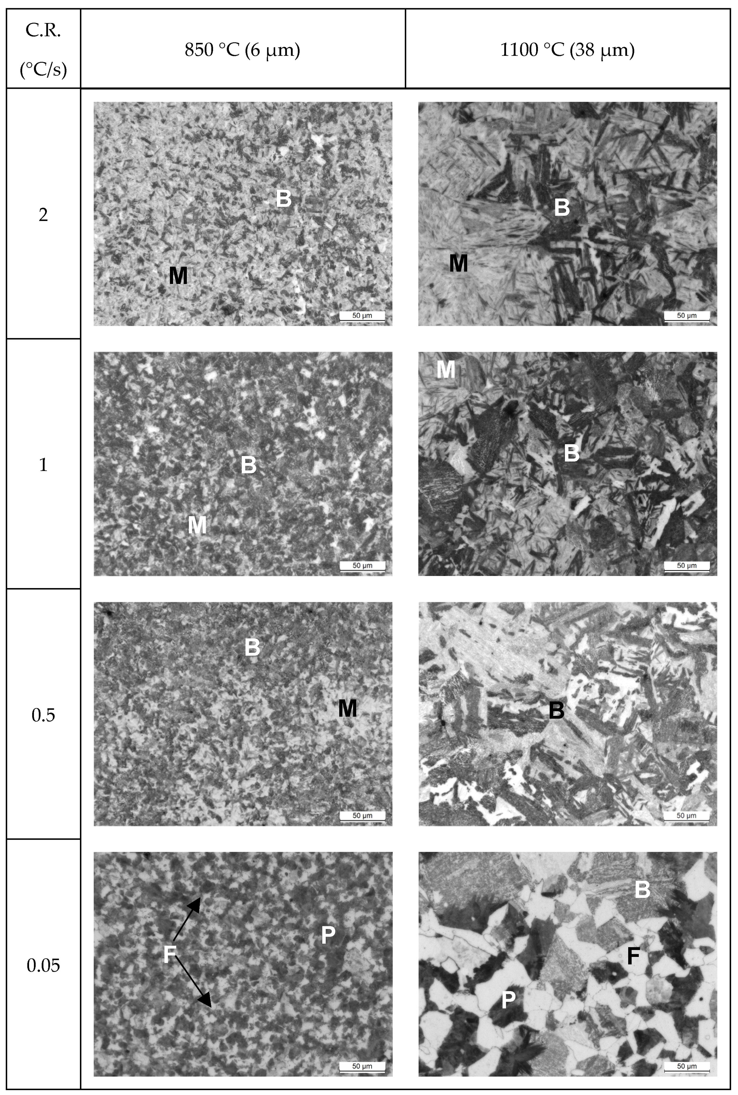
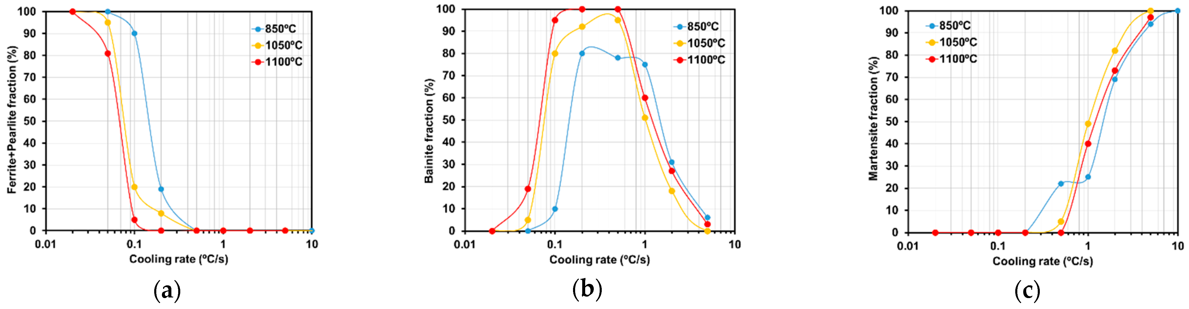
3.4. Microstructural Evolution

Optical micrographs taken for different cooling conditions and austenization temperatures are illustrated in Figure 9. The evolution of the microstructure with the cooling rates in the range 0.05 °C/s and 2 °C/s is characterized by the transition from mainly ferrite-pearlite microstructures to martensite-bainite ones. Only some bainitic zones are detected for 0.05 °C/s and the highest austenization temperature, 1100 °C.
The quantification of the microstructures is gathered in Figure 10 for each microstructural constituent, namely, ferrite-pearlite, bainite and martensite. The effect of the annealing temperature on the evolution of the different microconstituents with regard to the cooling rate can be summarized as follows. The ferrite-pearlite microstructures are favored at lower austenization temperatures. At cooling rates below 0.05 °C/s, the microstructure is fully ferritic-pearlitic for 850 °C, whereas bainite appears at that cooling rate, if the austenization temperature is 1050 °C or higher. Bainite is formed at intermediate cooling rates, between 0.1 °C/s and 2 °C/s, but the attained fraction is maximized at higher austenization temperatures. Particularly, after holding at 1100 °C, an almost fully bainitic structure is attained for such an intermediate cooling rate range. The critical cooling rate for bainite to start forming is delayed as lower austenization temperatures are applied.
As a general observation, the dilatometry signal and the microstructural quantifications agree. Even fractions as low as 5%, at 5 °C/s after austenitizing at 850 °C, can be detected.

3.5. Open-Source Software: Results for the Current Steel Grade

As detailed in the Introduction, there is a large number of different approaches to model phase transformation kinetics under isothermal, continuous cooling and anisothermal conditions. In this study, the open-source models based on Li’s approach, but with some additional improvements [24,26], were applied to predict either the transformation start temperatures or the fraction of the various microconstituents. It is noted that Nishikawa’s code [24] was slightly modified so as to consider the simultaneous phase transformation of ferrite and/or pearlite with bainite. This change did not have a significant impact on the final results for the present steel grade.
The predictions of the open-source models are gathered in Figure 11 for an austenization temperature of 1100 °C. For the sake of clarity, from this point on, the legends in the figures will contain a capital letter, N and C, that stand for Nishikawa’s model [24] or Collins et al.’s model [26], respectively. The results show that there are differences between the two models even though the approaches themselves are similar. The ferrite transformation kinetics are very similar for all the cooling rates. Instead, the bainitic reaction is affected by the applied model, leading to a deceleration of the bainite transformation for intermediate cooling rates in Collins et al.’s [26] model predictions.
Details of the reasons for such divergences are discussed thoroughly in the Section 4.

4. Discussion

This section concentrates on the modeling task of the work aiming at assessing the quality of the predictions in terms of quantitative results and improving Li’s approach-based models, accounting for the experimental results in a chemically heterogeneous 42CrMo4.

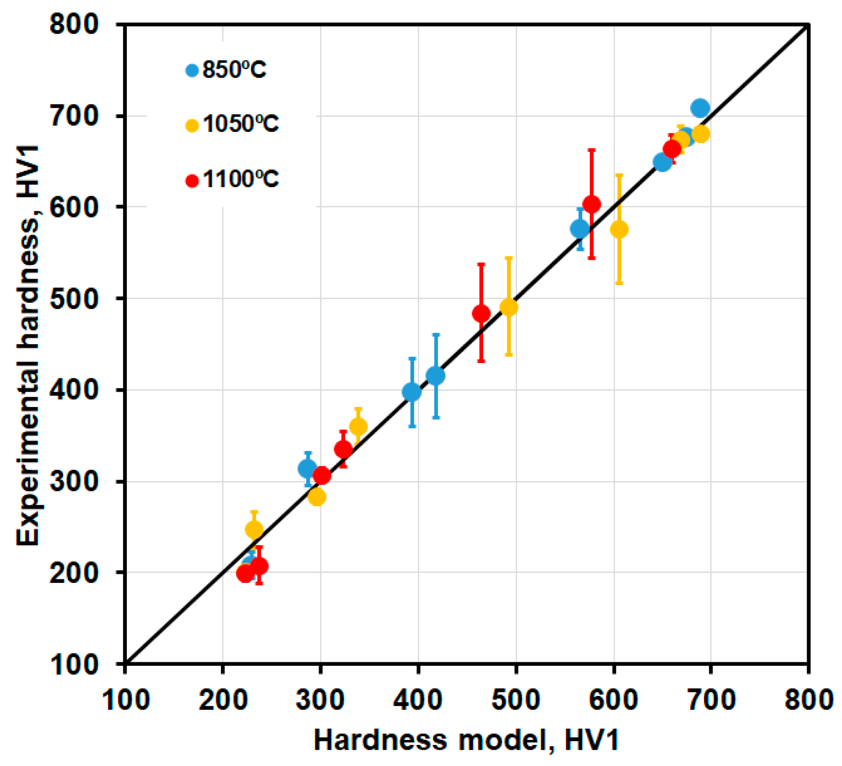
4.1. Modeling Hardness

The hardness in low alloy steels has been typically predicted through empirical models that relate hardness with the microconstituent fractions, chemical composition and cooling rate. For this study, the formulation proposed by Maynier et al. in [28], which has been proven to give reasonable predictions in the general literature [23], was used to predict hardness. The chemical composition in Table 1 together with the fractions determined experimentally, see Figure 10, are inputted. The comparison of the results of the model with experimental data is illustrated in Figure 12.
Even though the predictions rely on average chemical compositions, there is a nice agreement which validates this formulation for the present steel grade. The largest scatter in hardness is correlated with the bainite and martensite microstructure mixtures, where the material shows the more evident presence of the segregation pattern.

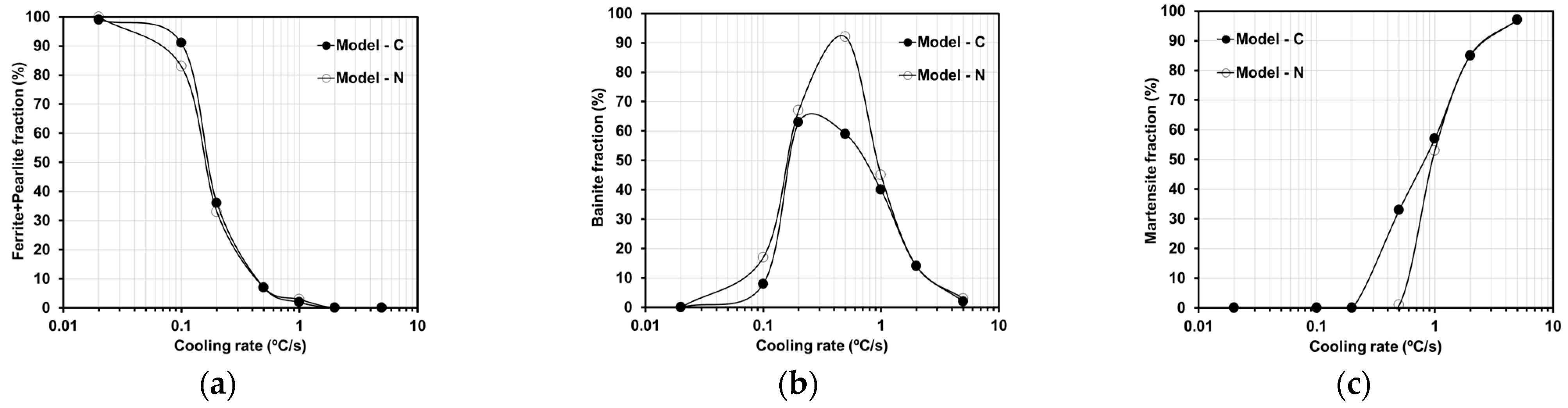
4.2. Modeling Phase Transformation

The direct comparison of the predictions of the open-source models as they are in their repositories [24,26] with the experimental start temperatures and microconstituents fractions are depicted in Figure 13. The main results are described next:
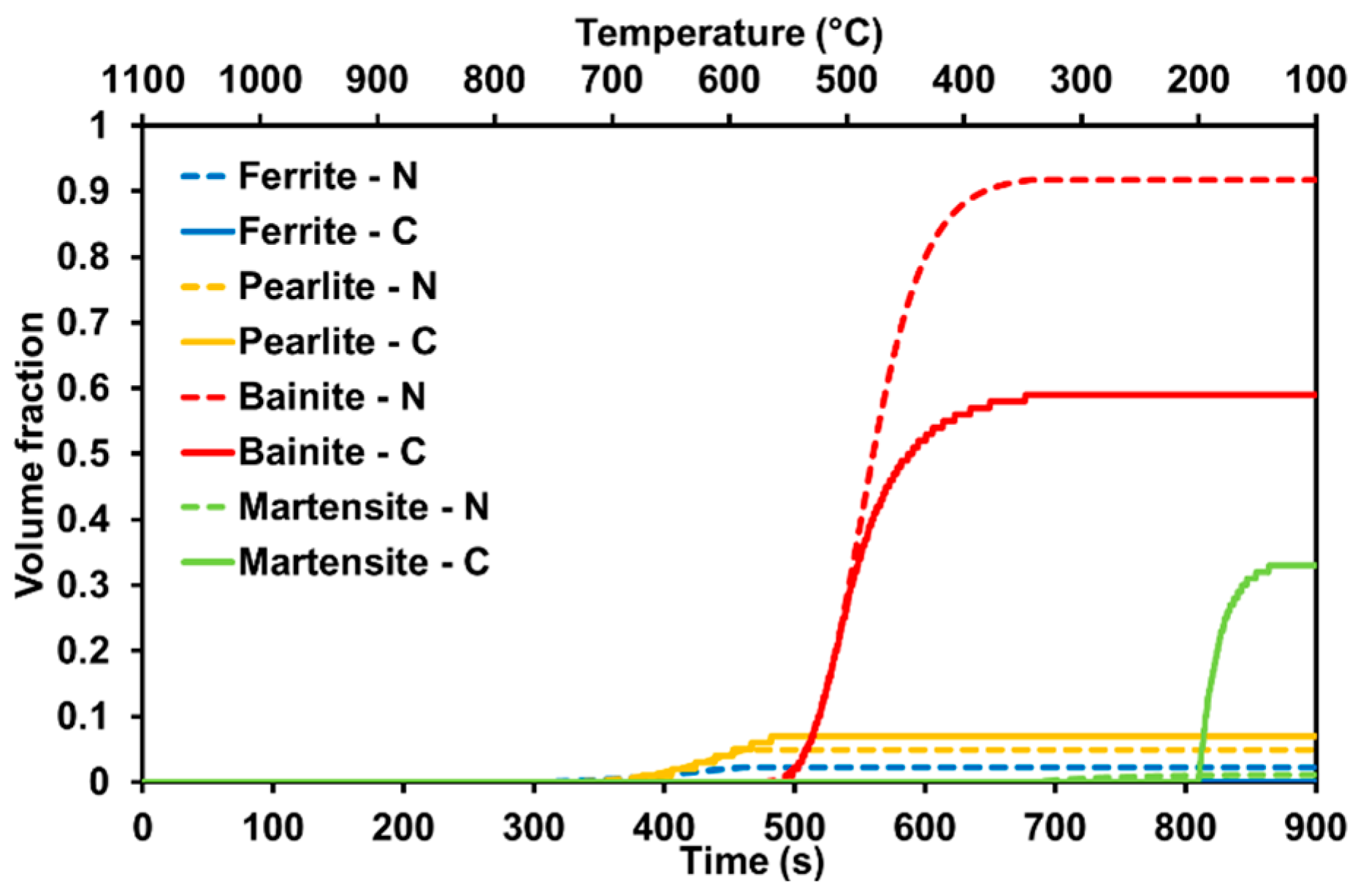
  • Significant changes in the prediction of the onset of ferrite-pearlite transformation depending on the model. Instead, the bainite and martensite start temperatures of the two models are close. In general, Nishikawa’s formulation [24] agrees better with the experimentally determined temperatures for ferrite, whereas Collins et al.’s [26] formulation excels when it comes to the bainite and martensite start temperature.
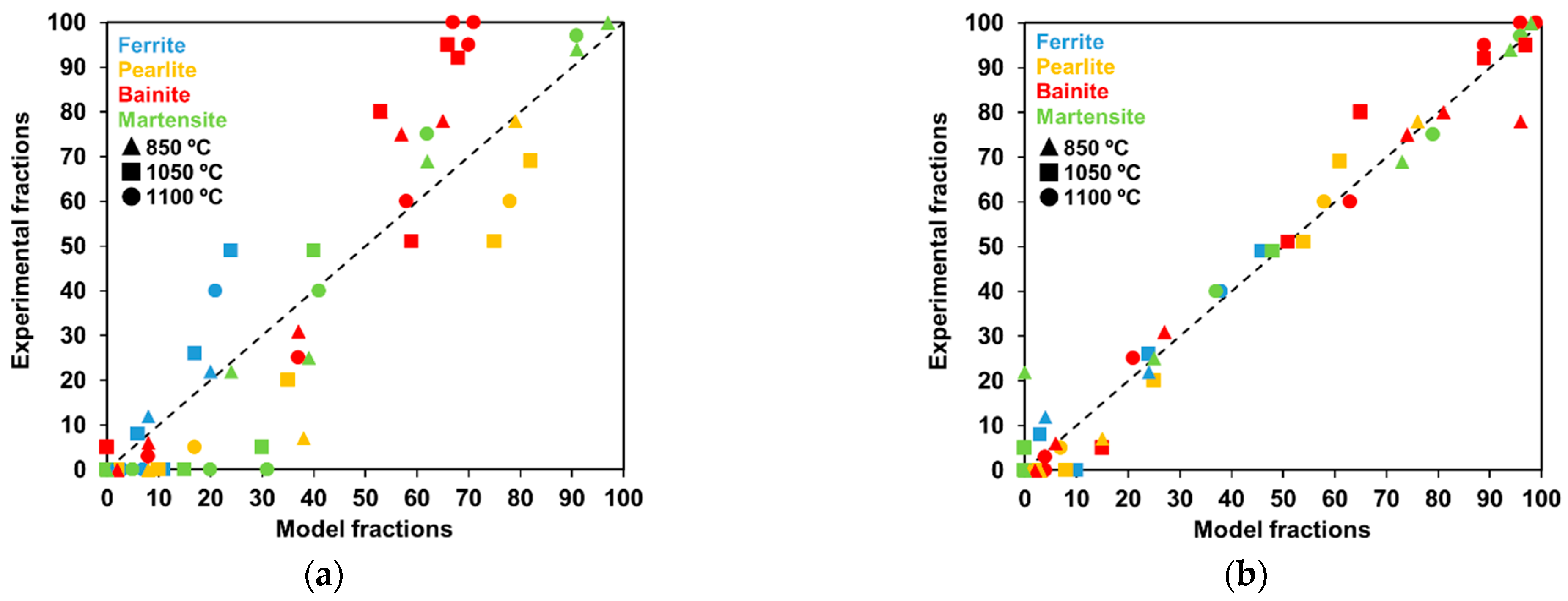
  • However, looking at the phase fractions, the predictions largely deviate from the experimentally measured fractions of the different microconstituents regardless of the approach undertaken.
Figure 13. Comparison of the results of the different models after austenization at 1100 °C. (a) Start temperatures, assuming 1% of newly formed phase; (b) Fractions.
Metals 14 01096 g013
With the objective of grasping the reason for the deviations between models, some of the main features of the two approaches are summarized in Table 2. To begin with, the variation in the ferrite-pearlite start transformation temperatures is directly related to the use of different Ae3 and Ae1 formulations. However, the Bs formulation is common to both and, even though the integration schemes differ, the predictions for bainite transformation onset are close.
As far as volume fractions are concerned, the two models fail in predicting the measured fractions. As pointed out in Table 2, the critical temperatures (Ae1, Ae3, Bs, Ms) and the integration of Li’s approach are significantly different, leading to such divergence. This is clearly observed in the prediction of the two models with cooling time for the condition T a u s = 1100 °C and CR = −0.5 °C/s, under the assumption that the Ae3 and Ae1 temperatures are formulated by Grange’ equations in [29], Figure 14. The impact of the stagnation in the bainitic reaction as well as the decrease in the martensite start temperature is better described by Collins et al. model [26].
In the following subsections, several strategies are attempted to enhance the quality of the predictions of the models. Basically, the strategies are based on the improvement of the following:
Individual models;
Overall transformation model;
Introduction of the compositional heterogeneity in the model.
To make it easier to understand how the strategies just mentioned, which are built on the modifications of the kinetics of ferrite, pearlite and bainite transformations, are planned to be employed, the common function type describing such kinetics under isothermal conditions is defined as follows:
τ i X i , T , G ,   C o m p o = 2 N G P i C o m p o T i T n exp Q R T S X i
where τi is the time for the i-microconstituent to reach an X i transformed fraction, G is the austenite grain size in the ASTM number, T i is the critical temperature for the onset of transformation of austenite-to-i-microconstituent, P i is the composition-dependent term and S X i is the reaction rate term for the i-microconstituent. The latter is an approximation to the sigmoidal effect of phase transformations; refer to detailed description in [23].

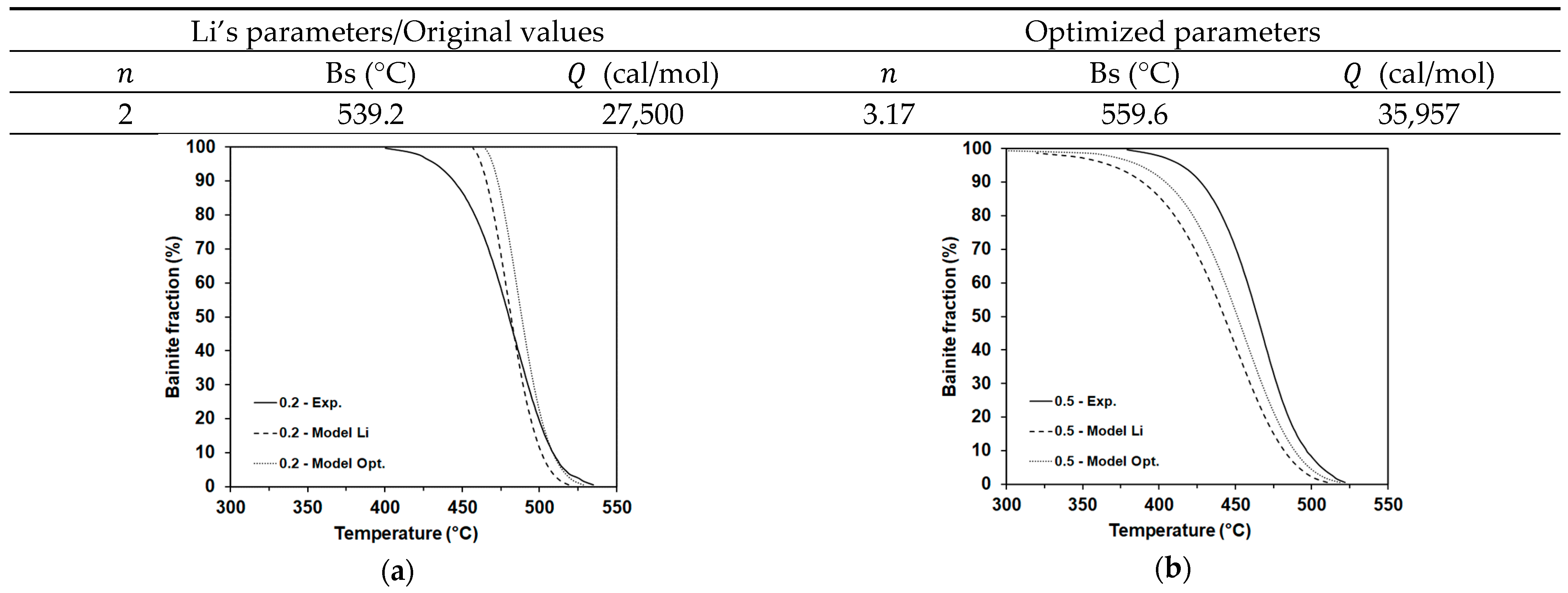
4.2.1. Improvement of the Transformation Models for Each Product Phase: Application to the Bainite Transformation Model

The quantitative results in Figure 10 allow selecting experimental conditions that yield a one-phase microstructure to analyze the transformation models for each product phase. In that regard, the goodness of the austenite to bainite transformation model was tested under continuous cooling conditions for an austenitizing temperature of 1100 °C and a cooling rate of 0.2 °C s−1 and 0.5 °C s−1, which led to almost fully bainitic microstructures. The experimental bainitic transformation kinetics are shown in Figure 15, which was determined by the application of the classical lever rule on the dilatation curve. Assuming a functional dependence of the bainitic transformation kinetics τ B X , T , G ,   C o m p o used by the open-source models, Equation (3), the sensitivity of the bainitic transformation kinetics to Bs, bainitic start transformation temperature, as well as to the n and Q value in the general expression was assessed through the optimization of these three values in Equation (3) by mean least square optimization methods.
τ B X B , T , G , C o m p o                                                     = 2 0.29 G exp ( 10.23 + 10.18 C + 0.85 M n + 0.55 N i + 0.9 C r                                                     + 0.36 M o ) Bs   T n exp Q R T S X B
The shape predicted by the Li-type Kirkaldy model, using the original values indicated in the table inserted in Figure 15, does not fit the actual experimental curves regardless of the applied parametrization, Figure 15a,b. This is certainly evident in the region where the kinetics speeds up, which corresponds approximately to the zone of 20% to 80% bainitic transformation. Figure 15a,b, additionally, display a comparison between experimental bainitic transformation and the optimized modeled one. It can be observed how the optimized model fails to capture the bainite transformation kinetics.

4.2.2. Improvements in the Overall Open-Source Models

To improve the quantitative predictions of the phase transformation model, two aspects may be considered for the fine-tuning of the parameters. On the one hand, the various transformation start/finish temperatures can be regarded as the objective. On the other hand, the fractions of the microconstituents may be used to fit the parameters accordingly. Recently, Rauch et al. [33] have defined a function to be minimized, Equation (4), in which all parameters are considered but assuming different weights for each parameter.
Φ a , p = w T n i = 1 n T i m T i c T m 2 + w X k i = 1 k X i m X i c X i m 2
where T i m and T i c are the measured and calculated start and end phase transformation temperatures, X i m and X i c are the measured and calculated volume fractions of the phases after cooling and n and k are the number of measurements of temperatures and volume fractions of phases. Finally, w T and w X are the weight or each set of parameters. The best method to solve this kind on inverse problem was found to be the Particle Swarm Optimization (PSO) in Ref. [33] that takes into account different seeds in the optimization task for parametrization. The specifications and details of the application of the PSO to the current analysis are given in Appendix B. Trying to keep it as simple as possible, the main efforts were focused on the fractions, presented in Figure 10, ruling out the start and end phase transformation temperatures in the optimization process. Additionally, the weighting factors were set to 1 and, the compositional P i C o m p o and grain size 2 N G , dependent functions in Equation (2), were calculated as one for each microconstituent (ferrite, pearlite, bainite). That is to say, the temperature-related terms were maintained in the original form and grain size and compositional terms were put together as only one value for each microconstituent. The numerical results of those terms are collected in Table 3, after applying the customization of the PYSWARM toolkit [34] for the present problem.
The results of such an approach are gathered in Figure 16. The improvement of the model is remarkable, compared to results in Figure 13b, and the scatter of the data around the 1:1 relationship remains relatively low. In particular, using RMSE (root mean square error) to measure the goodness of the models, its value for Nishikawa’s approach is 0.046, whereas for Collins’ approach, it is 0.122.

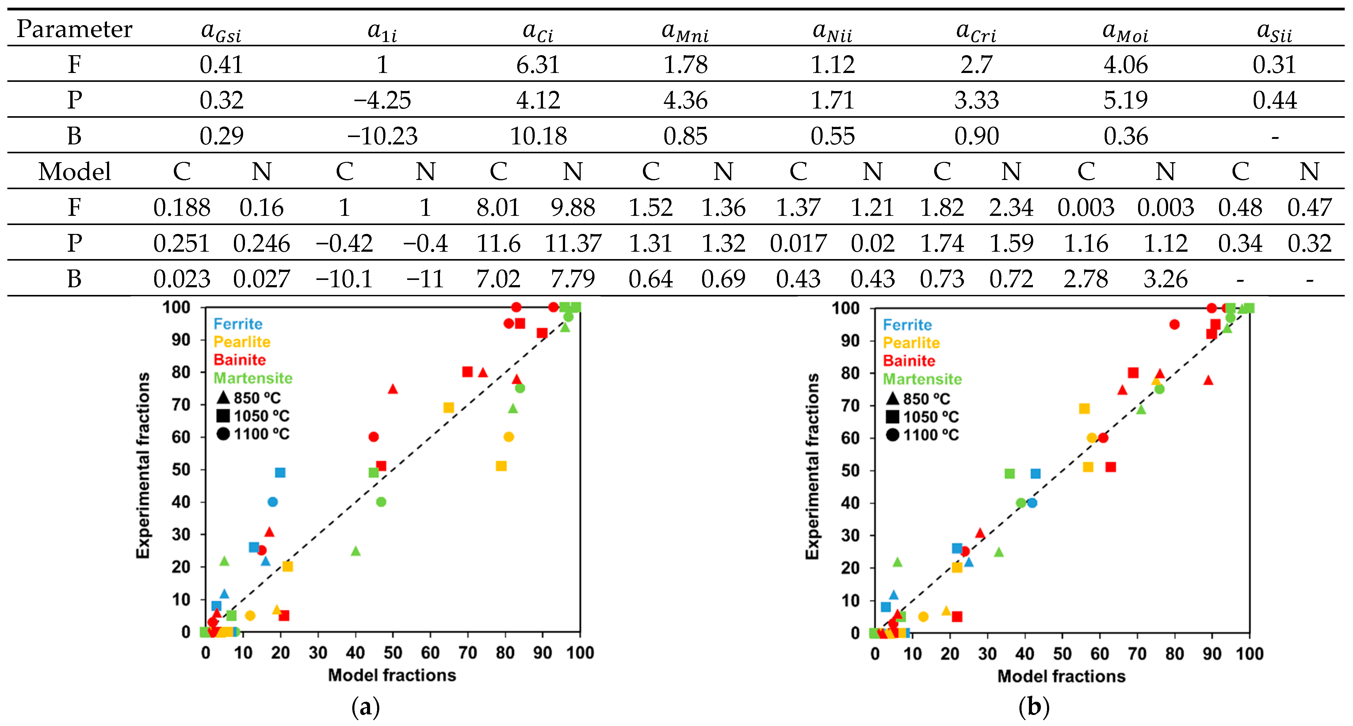
4.2.3. Sensitivity to the Chemical Composition: Introduction of the Heterogeneity in the Modeling of the Phase Transformation of 42CrMo4 Steel

Up to now, the discussion has relied on the mean chemical composition of the steel. However, the material shows large heterogeneities in the microstructure as a consequence of the different thermal cycles and chemical segregations. The open-source software allows introducing in a simple way the chemical heterogeneities in the continuous cooling simulations. Aiming to account for the chemical heterogeneity in the present analysis, EDS linescans were performed on a set of samples to characterize the chemical heterogeneity, specifically, in samples cooled at −1 °C/s from the two austenization temperatures, 850 °C and 1100 °C. The quantitative data, derived from those microanalyses, were obtained according to the methodology described in Appendix A. The original open-source models weree applied to the linescans in a point-to-point manner to calculate the volume fractions for some lines. Both models yielded an RMSE value of about 0.26. This value is close to the one achieved after the application of the original models to the nominal composition (RMSE ≅ 0.27).
Finally, the PSO approach was deployed, assuming that the linescans were illustrative of the general chemical heterogeneity of the material. The optimized parameters, which were previously evaluated for the models under homogeneous conditions, demonstrated difficulties in capturing the effect of the heterogeneity. In light of this limitation, a new methodology was introduced to improve the quality of the predictions. Specifically, the PSO algorithm was applied on the chemical profile (heterogeneity) and grain size terms of Li’s approach, but this time the vector of parameters a X i , as expressed in Equation (5), was the object for optimization of the phase transformation model, where X and i stood for the different chemical elements and i-microconstituents (ferrite, pearlite or bainite), respectively.
P i C o m p o = exp ( a 1 i + a C i   % C + a M n i   % M n + a N i i   % N i + a C r i   % C r + a M o i   % M o + a S i i   % S i ) 2 a G s i   G
Li’s original work and optimized compositional parameters calculated in this work together with the comparison of the experimental and model results are shown in Figure 17.
To wrap up, the RMSE parameter change, depending on the strategy and model, is illustrated in Table 4. There are some clear results that will be described next. First, Nishikawa’s approach performs better than Collins et al.’s when heterogeneity is considered. The application of optimization strategies to the two approaches yields a much lower RMSE than the original ones. Finally, the introduction of the heterogeneity in the models brings about a decrease in the RMSE value.

4.3. Limitations

There are still many missing points to be tackled by Kirkaldy’s kind of models to achieve reliable predictions. A nicely reported description of these issues is written in [25], indicating the inherent limitations in Li’s original approach: (a) the accuracy of the original Li predictions due to the empirical nature of the models, (b) the empirical source data used to calibrate their predictions. As stated by those authors for their model [25], “Although improvements were made to the CCT predictions, the accuracy of the proposed model is restricted by the inherent, empirical limitations of the original semi-empirical expressions. Correcting these limitations would require developing new sets of constituent transformation expressions around reliable and carefully controlled TTT and CCT datasets”. In the present work, the application of optimization methods for the improvement of Li’s approach to predict the phase transformation on a set of CCT curves of a chemically heterogeneous 42CrMo4 steel is analyzed. As expected, a consistent model that predicts simultaneously the start and end temperatures of phase formation and the volume fractions of the various phases is not accomplished when the basic structure of Li-type formulations is applied. The main reason lies in applying the nominal chemistry of the steel in a chemically segregated (heterogeneous) 42CrMo4 steel, even though optimized parameters are included. The same issue is also true when the individual models are regarded. Trying to overcome this issue, the application of the optimization tools for parameter identification in the case of heterogeneous compositions was explored. Other sources of disagreement can be also found:
  • The formulation for the transformation onset (Ae1, Ae3, Acm, Bs, etc.) of the different austenite products can strongly affect the predicted volume fractions.
  • The strategy applied to integrate the full transformation model may lead to significant scatter in the results. It must be recalled that the model has to deal with conditions under which multiple transformation products are formed. From the results above, the introduction of some physical considerations (Collins et al.) or the simple possibility to transform austenite into more than one microconstituent at every integration step (Nishikawa) in the models bring about variations in the optimized parameter values. This is clearly proven in Table 3, where the values are significantly different for each model.
  • The linear approaches to the composition-dependent term do not reflect likely higher-order correlations or some synergistic effects on phase transformations, which are usually reported in the literature [35].
  • Lastly, the chemical characterization at the micro/mesoscale of the samples is of crucial significance since it is the base for properly describing the behavior of the phase transformations while being closer to the actual observed phenomena.

5. Conclusions

5.1. Experimental Characterization

The present work gives a detailed dilatometry study of the phase transformation of 42CrMo4 steel arising from an industrial material characterized by its chemical heterogeneity. Several conclusions can be extracted from the experimental characterization. Looking at the CCT curves, the change in the austenization temperature (grain size) has a marked impact on the ferrite-pearlite transformation region. Instead, the shape and extension, in terms of cooling rates, of the bainitic transformation region is less affected. This may be attributed to the chemical heterogeneity, which may dilute the effect of the grain size on bainitic transformation kinetics. With regard to the microstructure development, large enough grain sizes, after austenization at 1100 °C, generate almost completely bainitic structures in a certain range of continuous cooling rates, 0.1 to 0.5 °C/s. However, the formation of fully martensitic microstructures, often aimed at 42CrMo4 steel grade, is attainable if cooling rates higher than 5 °C/s are applied.

5.2. Modeling Phase Transformation upon Continuous Cooling

The present work tries to improve the quality, in terms of quantitative measures, of the phase transformation predictions of two already developed CCT modeling formulations (Nishikawa and Collins et al.) based on Li’s former phenomenological work when applied to heterogeneous chemical composition in a 42CrMo4 steel. The way the different phenomena are modeled or the way the integration scheme is considered when multiple phases are formed, which make the difference between the formulations, may induce variations in the predictions. The predictions of the two approaches are far from the experimental observations when nominal chemistry is used, as RSME values over 0.25 are obtained irrespective of the model and chemical spatial distribution. The use of different strategies that embrace improvement of the individual models for each austenite product, a new minimization formulation for parameter fitting and, finally, heterogeneity conditions is tackled. In particular, the introduction of the spatial chemical heterogeneity adds complexity to the modeling task. The need for an accurate characterization of the chemical spatial distribution, diffusion simulation tools (DICTRA in this work) and optimization tools for fine-tuning of the parameters of the phenomenological models is shown in this work. In the present study, RSME values below 0.09 are achieved for the two formulations when considering the optimized parametrization as well as the chemical heterogeneity.
From the results of this work, it is foreseen that the use of chemically heterogeneous materials together with appropriate modeling and microstructure/chemical characterization tools may be a way to accelerate the development of new phenomenological phase transformation models.

Author Contributions

Conceptualization, D.J.-B. and A.I.-M.; methodology, D.J.-B. and S.F.-S.; validation, D.J.-B. and S.F.-S.; formal analysis, D.J.-B., A.I.-M. and S.F.-S.; resources, D.J.-B. and A.I.-M.; data curation, S.F.-S.; writing—original draft preparation, D.J.-B.; writing—review and editing, D.J.-B., A.I.-M. and S.F.-S.; visualization, D.J.-B. and S.F.-S.; supervision, D.J.-B. and A.I.-M.; project administration, D.J.-B.; funding acquisition, D.J.-B. and A.I.-M. All authors have read and agreed to the published version of the manuscript.

Funding

This work has been granted by Basque Governmental Research Program ELKARTEK through MEEVCE project KK-2022/00105 and MEEVCE II project KK-2024/00047.

Data Availability Statement

The datasets presented in this article are not readily available because the data are part of an ongoing study. Requests to access the datasets should be directed to the authors.

Acknowledgments

Special thanks are addressed to Itziar Morán Magariño for her work in the laboratory tasks as well as her insightful comments on the experimental observations.

Conflicts of Interest

The authors declare no conflicts of interest.

Appendix A. Description of the Chemical Heterogeneity

The chemical heterogeneity of the material under analysis has been characterized by EDS (electron dispersive spectroscopy) by using the AzTec software. The quantification carried out with this software is based on the simultaneous application of the following techniques in the standardless mode: QCAL, FLS, XPP and Pulse Pile-Up Correction. QCAL technology is a quantitative calibration approach that delivers a unique set of parameters and an efficiency curve for each hardware type; FLS is the Filtered Least Squares Fitting for the background correction; XPP is the Exponential model of Pouchou and Pichoir Matrix Correction [36].
The analyses were performed under the conditions gathered in Table A1 on lines that cross several dendrites as observed in Figure 4a. Those lines were randomly distributed over the selected samples: T a u s = 850 °C and 1100 °C and C.R. = −1 °C/s. The number of lines was five per condition.
Table A1. Conditions applied for setting up the EDS analyses at ZEISS Σ500 FEG-SEM microscope.
Microscopy ConditionsAcquisition Conditions
Potential (kV)20Step/total line length (μm)3–5/1400–2800
Dwell time (ms)1500
Aperture (μm)60 (High Current)Analyzed elementsFe-Cr-Mn-Si-Ni-Cu
The microchemical quantification was carried out taking into account the next spectral lines for each element: Fe (Kline), Cr (Kline), Mn (Kline), Mo (Lline), Ni (Kline) and Si (Kline). The results were normalized to 100% for such quantification.
In order to smooth out likely spurious/artificial peaks, the chemical composition at each point was calculated by averaging over the 30 μm length. An example of a quantitative linescan is shown in Figure A1, where only the elements that contribute to the kinetics of the phase transformations in the original work by Li et al. [23], except for C, are illustrated. In this particular case, the presence of a peak in the amount of Cr and Mn at about 600 μm is readily observed in Figure A1.
Figure A1. An example of a linescan showing the chemical changes.
Metals 14 01096 g0a1
The details of the statistical analysis are gathered in Table A2, in which the chemical information is given in a point-to-point or line-to-line manner. In order words, the statistical samples are the points in all lines or the lines themselves, respectively. In general, the EDS measurements, in the mean chemical composition EDS row, are slightly higher than the ones measured through the AES (Atomic Emission Spectroscopy) technique. The experimental point-to-point chemical analysis scatters due to the inherent experimental error and the spatial chemical heterogeneity itself. However, the significantly wider range of chemical compositions attained per line, Amplitude EDS (95% data interval), than the amplitude considering the mean composition of all the analyzed lines makes it reasonable to use them as the measure of the heterogeneity.
Table A2. Comparison of the chemical composition determined through AES and EDS of the main elements.
ElementCMnSiCrMoNi
Chemical composition (AES)0.440.740.221.020.240.14
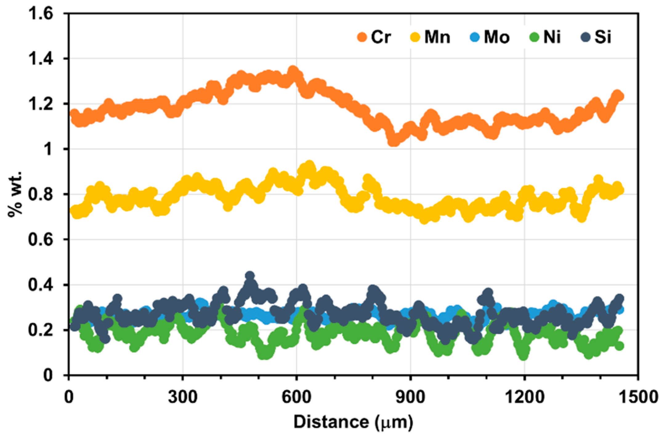
Mean chemical composition based on all EDS spectra (point-to-point)Unknown0.820.261.170.280.16
Amplitude EDS per element based on all EDS spectra (95% data interval, point-to-point)Unknown0.080.060.120.080.07
Amplitude of mean EDS among all lines (Max-Min)/2 (line-to-line)Unknown0.060.010.030.030.04
Taking into account these observations, the mean chemical composition for each line was calculated and the difference with regard to actual value per point was estimated for all elements except for C. Then, this difference was added to the nominal composition (chemical composition (AES)) at each scanned point. However, as discussed in [36] for EPMA (Electron Probe MicroAnalyzer), but also applicable to EDS analyses, C pollution masks the real C content. Based on the approach undertaken in [37], the C profile was determined for the different lines with the help of DICTRA (Thermo-Calc Software AB Råsundavägen, Solna, Sweden) with TCFE10 and MobFe7 databases. These experimentally characterized chemical profiles account for the likely common segregation of some elements. As an example, a typical chemical distribution line is given in Figure A2a. Two extreme initial scenarios for C distribution before austenization stage were analyzed:
  • C distributes homogeneously (constant value of 0.44%).
  • C distributes as if the material was held for a very long time (half a day) at a temperature of 1250 °C (simulating the solution heat treatment before high temperature thermomechanical processing).
The results of the carbon distribution do not deliver highly different patterns depending on the scenario, and the C minimum and maximum are in the range 0.43 and 0.45%, Figure A2b.
Figure A2. Distribution of (a) the main elements on a line analyzed in sample 850 °C and (b) carbon upon different initial conditions calculated with DICTRA. (a) Homogeneous (0.44%C) and (b) After solution heat treatment at 1250 °C for 0.5 days.
Metals 14 01096 g0a2
Additionally, the correlation matrix for the chemical elements was determined, Table A3. The results show that the Mn-Cr-Mo elements tend to be correlated as the Pearson correlation coefficients are typically greater than 0.6. This is a sign of common segregation of such chemical species in the steel under study.
Table A3. Correlation matrix (Pearson correlation coefficient) for analyzing the chemical segregation.
Chemical
Element
Cr
Cr1.000Mn
Mn0.7011.000Mo
Mo0.6550.6181.000Ni
Ni0.0480.1220.0321.000Si
Si0.2040.5150.132−0.0091.000

Appendix B. Description Particle Swarm Approach

Least squares optimization methods have been observed to struggle when tuning the parameters within compositional terms. The employment of metaheuristic algorithms has emerged as a viable solution to address this task. Particle Swarm Optimization (PSO) is a metaheuristic computational method that imitates social behavior to search for optimal global solutions for a given problem.
PSO is initialized by generating a population of random solutions. Each of these potential solutions are called “particles”, and they keep track of their respective coordinates within the problem space throughout all the iterations performed in the PSO. Every coordinate can be associated with the goodness of the solution given by itself. In this study, the goodness was evaluated by measuring the error of the consequent phase fractions calculated with the model. Thus, at each step t , the best potential solution achieved by every particle is known, which is commonly noted as p b e s t i t for particle i . Additionally, the global best potential solution obtained at step t , is noted as g b e s t t .
The concept of PSO follows a very basic procedure of updating the position of every particle at each time step by changing its velocity toward both its respective and global best solutions. This behavior is expressed as follows:
x i t + 1 = x i t + v i t + 1 , v i t + 1 = w v i t + c 1 r 1 p b e s t i t x i t + c 2 r 2 g b e s t t x i t , i     1 ,   2 ,   ,   S ,   t     1 ,   2 ,   ,   t f ,
where x i t and v i t are the coordinates and velocities of the particle i at time step t , S is the number of particles in the swarm and t f is the number of steps followed during the optimization. The terms r 1 and r 2 are randomly generated and both of them follow a uniform U 0 , 1 distribution. The coefficients w ,   c 1 ,   c 2 are shared across all particles in the optimization and play a pivotal role in its functioning. The coefficient w governs the inertia, while c 1 and c 2 determine the influence of cognitive and social behaviors, respectively, for each particle.
Typically, the stopping criterion involves reaching a determined number of iterations, at which point, the best solution found ( g b e s t t f ) is returned as the optimized value.
There is no clear consensus on which coefficients to use in the optimization. While particle sizes of 20–50 are a common choice for sufficiently good solutions and a minimized number of evaluations [38,39], certain studies utilizing meta-optimization have indicated that larger particle sizes lead to improved convergence for specific problem instances [40,41]. The variability observed in the values of S extends to the coefficients w   ,   c 1 ,   c 2 , thereby underscoring the problem-specific characteristics inherent in the PSO coefficients. The coefficients employed in this study primarily comprise S = 50 , w = 0.729 , c 1 = c 2 = 1.494 , although alternative values have been also explored.

References

  1. Bhagyalaxmi; Sharma, S.; Jayashree, P.K.; Hegde, A. Vegetable oil quench effect on impact toughness and hardness of 42CrMo4 steel. Mater. Today Proc. 2022, 63, 113–116. [Google Scholar] [CrossRef]
  2. Abdul Khadeer, S.; Ramesh Babu, P.; Ravi Kumar, B.; Seshu Kumar, A. Evaluation of friction welded dissimilar pipe joints between AISI 4140 and ASTM A 106 Grade B steels used in deep exploration drilling. J. Manuf. Process. 2020, 56 Pt A, 197–205. [Google Scholar] [CrossRef]
  3. Costa, L.L.; Brito, A.M.G.; Rosiak, A.; Schaeffer, L. Microstructure evolution of 42CrMo4 during hot forging process of hollow shafts for wind turbines. Int. J. Adv. Manuf. Technol. 2020, 106, 511–517. [Google Scholar] [CrossRef]
  4. Gramlich, A.; Hinrichs, T.; Springer, H.; Krupp, U. Recycling-Induced Copper Contamination of a 42CrMo4 Quench and Tempering Steel: Alterations in Transformation Behavior and Mechanical Properties. Steel Res. Int. 2023, 94, 2200623. [Google Scholar] [CrossRef]
  5. Smokvina Hanza, S.; Stic, L.; Liveri, L.; Spada, V. Corrosion behaviour of tempered 42CrMo4 steel. Mater. Technol. 2021, 55, 427–433. [Google Scholar] [CrossRef]
  6. Xu, Q.; Liu, Y.; Lu, H.; Liu, J.; Cai, G. Surface Integrity and Corrosion Resistance of 42CrMo4 High-Strength Steel Strengthened by Hard Turning. Materials 2021, 14, 6995. [Google Scholar] [CrossRef]
  7. Behrens, B.A.; Brunotte, K.; Petersen, T.; Diefenbach, J. Mechanical and Thermal Influences on Microstructural and Mechanical Properties during Process-Integrated Thermomechanically Controlled Forging of Tempering Steel AISI 4140. Materials 2020, 13, 5772. [Google Scholar] [CrossRef]
  8. Zhu, J.G.; Sun, X.; Barber, G.C.; Han, X.; Qin, H. Bainite Transformation-Kinetics-Microstructure Characterization of Austempered 4140 Steel. Metals 2020, 10, 236. [Google Scholar] [CrossRef]
  9. Park, J.S.; Kim, S.W.; Lee, H.W.; Han, K.B.; Lee, J.M.; Kang, J.H. Hardness Prediction of Wind Turbine Components Considering the Tempering Effect. Int. J. Eng. Trends Technol. 2022, 70, 57–62. [Google Scholar] [CrossRef]
  10. Nabil, M.; Taha, O.; Elbitar, T.; El Mahallawi, I. Thermomechanical processing of 42CrMoS4 steel. Int. Heat Treat. Surf. Eng. 2013, 4, 87. [Google Scholar] [CrossRef]
  11. Hunkel, M. Segregations in Steels during Heat Treatment—A Consideration along the Process Chain. HTM J. Heat Treat. Mater. 2021, 76, 79–104. [Google Scholar] [CrossRef]
  12. Gutman, L.; Kennedy, J.R.; Roch, F.; Marceaux dit Clément, A.; Salsi, L.; Cauzid, J.; Rouat, B.; Combeau, H.; Založnik, M.; Zollinger, J. Characterisation of mesosegregations in large steel ingots. Proc. IOP Conf. Ser. Mater. Sci. Eng. 2023, 1274, 012049. [Google Scholar] [CrossRef]
  13. Krauss, G. Solidification, segregation, and banding in carbon and alloy steels. Metall. Mater. Trans. B 2003, 34, 781. [Google Scholar] [CrossRef]
  14. Abraham Mathews, J.; Sietsma, J.; Petrov, R.H.; Santofimia, M.J. Austenite formation from a steel microstructure containing martensite/austenite and bainite bands. J. Mater. Res. Technol. 2023, 25, 5325. [Google Scholar] [CrossRef]
  15. Kuziak, R.; Pidvysots’kyy, V.; Pernach, M.; Rauch, Ł.; Zygmunt, T.; Pietrzyk, M. Selection of the best phase transformation model for optimization of manufacturing processes of pearlitic steel rails. Arch. Civ. Mech. Eng. 2019, 19, 535. [Google Scholar] [CrossRef]
  16. Vasilyev, A.A.; Sokolov, D.F.; Kolbasnikov, N.G.; Sokolov, S.F. Modeling of the γ→α Transformation in Steels. Phys. Solid State 2012, 54, 1669. [Google Scholar] [CrossRef]
  17. Kumar, M.; Sasikumar, R.; Kesevan Nair, P. Competition between nucleation and early growth from austenite- Studies using cellular automaton simulations. Acta Mater. 1998, 46, 6291. [Google Scholar] [CrossRef]
  18. Liu, Y.; Wang, D.; Sommer, F.; Mittemeijer, E.J. Isothermal austenite–ferrite transformation of Fe–0.04at.% C alloy: Dilatometric measurement and kinetic analysis. Acta Mater. 2008, 15, 3833. [Google Scholar] [CrossRef]
  19. Erişir, E.; Bilir, O.G. Phase Field Modeling of Microstructure Evolution during Intermediate Quenching and Intermediate Annealing of Medium-Carbon Dual-Phase Steel. In Proceedings of the Supplemental Proceedings 144th Annual Meeting & Exhibition TMS, Orlando, FL, USA, 15–19 March 2015; pp. 1433–1440. [Google Scholar]
  20. Iung, T.; Kandel, M.; Quidort, D.; de Lassat, Y. Physical modelling of phase transformations in high strength steels. Metall. Res. Technol. 2003, 100, 173–181. [Google Scholar] [CrossRef]
  21. Retz, P.; Shan, Y.V.; Sobotka, E.; Vogric, M.; Wei, W.; Povoden-Karadeniz, E.; Kozeschnik, E. Progress of Physics-based Mean-field Modeling and Simulation of Steel. Berg Huettenmaenn Monatshefte 2022, 167, 15–22. [Google Scholar] [CrossRef]
  22. Geng, X.; Wang, H.; Xue, W.; Xiang, S.; Huang, H.; Meng, L.; Ma, G. Modeling of CCT diagrams for tool steels using different machine learning techniques. Comput. Mater. Sci. 2020, 171, 109235. [Google Scholar] [CrossRef]
  23. Li, M.V.; Niebuhr, D.V.; Meekisho, L.L.; Atteridge, D.G. A Computational Model for the Prediction of Steel Hardenability. Metall. Mater. Trans. B 1998, 29, 661–672. [Google Scholar] [CrossRef]
  24. Nishikawa, A. Transformations Diagrams. 2020. Available online: https://github.com/arthursn/transformation-diagrams (accessed on 18 July 2023).
  25. Collins, J.; Piemonte, M.; Taylor, M.; Fellowes, J.; Pickering, E. A Rapid, Open-Source CCT Predictor for Low-Alloy Steels, and Its Application to Compositionally Heterogeneous Material. Metals 2023, 13, 1168. [Google Scholar] [CrossRef]
  26. Collins, J. Low Alloy Steel CCT Predictor. 2023. Available online: https://zenodo.org/record/776762 (accessed on 19 June 2023).
  27. Bach, F.W.; Schaper, M.; Yu, Z.; Nürnberger, F.; Gretzki, T.; Rodman, D.; Springer, R. Computation of isothermal transformation diagrams of 42CrMo4 steel from dilatometer measurements with continuous cooling. Int. Heat Treat. Surf. Eng. 2010, 4, 171–175. [Google Scholar] [CrossRef]
  28. Maynier, P.; Dollet, J.; Bastien, P. Prediction of Microstructure via Empirical Formulae Based on CCT Diagrams, Hardenability Concepts With Applications to Steel; The Metallurgical Society of AIME: San Ramon, CA, USA, 1978; pp. 163–178. [Google Scholar]
  29. Grange, R.A. Estimating Critical Ranges in Heat Treatment of Steels. Met. Prog. 1961, 79, 73–75. [Google Scholar]
  30. Kung, C.Y.; Rayment, J.J. An Examination of the Validity of Existing Empirical Formulae for the Calculation of Ms Temperature. Metall. Trans. A 1982, 13A, 328–331. [Google Scholar] [CrossRef]
  31. Andrews, K.W. Empirical formulae for the calculation of some transformation temperatures. J. Iron Steel Inst. 1965, 203, 721. [Google Scholar]
  32. van Bohemen, S.M.C. Bainite and martensite start temperature calculated with exponential carbon dependence. Mater. Sci. Technol. 2012, 28, 487–495. [Google Scholar] [CrossRef]
  33. Rauch, L.; Bachniak, D.; Kuziak, R.; Kusiak, J.; Pietrzyk, M. Problem of Identification of Phase Transformation Models Used in Simulations of Steels Processing. J. Mater. Eng. Perform. 2018, 27, 5725–5735. [Google Scholar] [CrossRef]
  34. Miranda, L.J. Pyswarms: A Research Toolkit for Particle Swarm Optimization. Available online: https://github.com/ljvmiranda921/pyswarms (accessed on 17 May 2024).
  35. Martin, H.; Amoako-Yirenkyi, P.; Pohjonen, A.; Frempong, N.K.; Komi, J.; Somani, M. Statistical Modeling for Prediction of CCT Diagrams of Steels Involving Interaction of Alloying Elements. Metall. Mater. Trans. B 2021, 52, 223–235. [Google Scholar] [CrossRef]
  36. Pouchou, J.; Pichoir, F. X-Ray Optics and Microanalysis; Brown, J., Packwood, R., Eds.; University of Western Ontario: London, ON, USA, 1987; p. 249. [Google Scholar]
  37. Ramesh Babu, S.; Ivanov, I.; Porter, D. Influence of Microsegregation on the Onset of the Martensitic Transformation. ISIJ Int. 2019, 59, 169. [Google Scholar] [CrossRef]
  38. Eberhart, R.C.; Yuhui, S. Particle Swarm optimization: Developments, Applications and Resources. In Proceedings of the 2001 Congress on Evolutionary Computation, Seoul, Republic of Korea, 27–30 May 2001; pp. 81–86. [Google Scholar]
  39. Meissner, M.; Schmuker, M.; Schneider, G. Optimized Particle Swarm Optimization (OPSO) and its application to artificial neural network training. BMC Bioinform. 2006, 7, 125. [Google Scholar] [CrossRef]
  40. Pedersen, M.E.H.; Chipperfield, A.J. Simplifying particle swarm optimization. Appl. Soft Comput. 2010, 10, 618. [Google Scholar] [CrossRef]
  41. Liao, Z.; Liu, Y.; Zhao, J. Meta-learning-based multi-objective PSO model for dynamic scheduling optimization. Energy Rep. 2023, 9, 1227. [Google Scholar] [CrossRef]
Figure 1. Equilibrium phase diagram calculated with Thermo-Calc (TCFe10 database) for composition in Table 1.
Metals 14 01096 g001
Figure 2. Evolution of the instantaneous cooling rate at different radial positions of a 42CrMo4 steel cylinder of ϕ = 1000 mm quenched in water. FE simulations.
Metals 14 01096 g002
Figure 3. Microstructure after etching with Nital 2%. (a) General optical picture of the whole dilatometry sample showing the heterogeneity. Optical micrographs corresponding to (b) dark regions and (c) bright regions. (d) FEG-SEM micrograph showing the detailed substructure of bainite and martensite. Sample after 850 °C–2 °C/s. B and M stand for bainite and martensite, respectively.
Metals 14 01096 g003
Figure 4. Optical micrographs of the previous austenite grain structure before final cooling. T a u s (a) 850 °C; (b) 1050 °C and (c) 1100 °C. Note that the magnifications are lower for 1100 °C. (d) Previous austenite grain size distribution for the three T a u s .
Metals 14 01096 g004
Figure 5. Correlation between (a) chemical pattern (nital etching) and (b) the austenite grain size (picric etching) for T a u s = 850 °C & C.R. = −5 °C/s. Mean equivalent diameter (M.E.D.) per region and austenization condition.
Metals 14 01096 g005
Figure 6. Comparison of the dilatation curve upon cooling at (a) −0.05 °C/s; (b) −0.5 °C/s; (c) −1 °C/s; (d) −2 °C/s.
Metals 14 01096 g006
Figure 7. CCT curve for the three T a u s .
Metals 14 01096 g007
Figure 8. (a) Hardness evolution and (b) Standard deviation of hardness with the cooling rate for the three T a u s .
Metals 14 01096 g008
Figure 9. Optical micrographs of the samples showing the transition from F + P microstructures to B + M microstructures for 2 austenization temperatures.
Metals 14 01096 g009
Figure 10. Evolution of the experimentally measured phase fractions as a function of the cooling rate for the three austenization temperatures (a) ferrite-pearlite; (b) bainite; (c) martensite.
Metals 14 01096 g010
Figure 11. Evolution of final volume fractions of each phase for the two models as a function of the cooling rate for T a u s = 1100 °C: (a) ferrite-pearlite; (b) bainite; (c) martensite.
Metals 14 01096 g011
Figure 12. Experimental vs. model hardness predictions.
Metals 14 01096 g012
Figure 14. Comparison of results of the simulations T a u s = 1100 °C (38 μm) at a cooling rate of −0.5 °C/s.
Metals 14 01096 g014
Figure 15. Application of the bainite model to the kinetics derived from the dilatation curve for cooling rates (a) 0.2 °C/s and (b) 0.5 °C/s.
Metals 14 01096 g015
Figure 16. Comparison of the model and experimental volume fractions for the two variants of Li’s original work after optimization of the grain size-compositional term for Collins et al.’s model (a) and Nishikawa’s (b).
Metals 14 01096 g016
Figure 17. Optimized compositional and grain size-related parameters for the two approaches and comparison of the experimental and predicted data after the optimization: (a) Collins et al.; (b) Nishikawa.
Metals 14 01096 g017
Table 1. Chemical composition of the steel grade 42CrMo4 (wt.%).
CMnSiCrMoNi
0.440.740.221.020.240.14
Table 2. Comparison of the main features of the open-source programs used in this work (as they are in [24,26]).
Open-Source SWIncluded Features (Integration Scheme)Omitted FeaturesCommon Features
Ae3Ae1BsMsTransformation Kinetics
J. Collins
[26]
  • Partitioning of C during γ to αf/B transformation
  • T0 temperature (bainite)
  • Bainite differentiation (Upper and Lower)
  • Simultaneous phase transformations are avoided
Grange
[29]
Grange [29]Li [23]Kung-Rayment [30]Original work by Li et al. [23]
A. Nishikawa [24]
  • Simultaneous phase transformation at any temperature
  • Chemical partitioning
  • T0 temperature (bainite)
  • Bainite differentiation (Upper and Lower)
Andrews [31]Andrews [31]Van Bohemen [32]
Table 3. Evaluation of the combined grain size-compositional term for Li’s original work and optimized for Nishikawa’s (N) and Collins et al.’s (C) approaches for ferrite, pearlite and bainite.
Taus (°C)Ferrite (Li)Ferrite (N/C)Pearlite (Li)Pearlite (N/C)Bainite (Li)Bainite (N/C)
8503302463/36793394/2800.00170.00355/0.0026
10508692975/490199571/5920.00340.00473/0.00254
110014655269/7902991203/8820.00490.00412/0.00261
Table 4. Evolution of the RMSE parameter depending on the model, type and chemical state.
ModelTypeChemicalRMSE
NOriginalHomogeneous0.271
COriginalHomogeneous0.271
NOriginalHeterogeneous0.263
COriginalHeterogeneous0.260
NOptimizedHomogeneous0.046
COptimizedHomogeneous0.122
NOptimizedHeterogeneous0.054
COptimizedHeterogeneous0.085
Disclaimer/Publisher’s Note: The statements, opinions and data contained in all publications are solely those of the individual author(s) and contributor(s) and not of MDPI and/or the editor(s). MDPI and/or the editor(s) disclaim responsibility for any injury to people or property resulting from any ideas, methods, instructions or products referred to in the content.

