Predictive Modeling and Optimization of Hot Forging Parameters for AISI 1045 Ball Joints Using Taguchi Methodology and Finite Element Analysis

Abstract

This study focused on optimizing the hot forging process for AISI 1045 medium carbon steel ball joints, which is crucial for enhancing both their mechanical properties and production efficiency. Traditional hot forging processes often face challenges due to variations in flow stress and microstructural outcomes, which can result in a suboptimal product performance. To address these challenges, this research employed the Taguchi method in conjunction with a finite element (FE) simulation to identify the optimal forging parameters. The Arrhenius constitutive model, based on the Zener–Hollomon parameter, was applied to predict the flow stress with a high level of accuracy, achieving a coefficient of determination (R²) of 0.968 and an average absolute relative error (AARE) of 7.079%. An analysis of variance (ANOVA), a statistical innovation that partitions the total variation into components linked to key process factors, was utilized to determine the significance of these parameters. The ANOVA revealed that the billet temperature played a significant role in influencing the preforming force, finishing force, and mean stress, with a maximum impact of 62.30%, 59.50%, and 94.20% on the variation in the response variable, respectively. Additionally, the friction factor significantly affected the preforming and finishing forces, contributing 36.19% and 38.28%. The validation of the model through both simulations and practical experiments is a testament to the reliability of this research, demonstrating the accuracy of the model with minimal discrepancies in the forging forces and exhibiting errors of just 2.88% and 3.40%. Furthermore, microstructure modeling successfully predicted the key outcomes, such as the grain size and pearlite volume fraction, validating the effectiveness of the simulation in forecasting microstructural characteristics.

1. Introduction

Hot forging, among all the manufacturing processes, stands out as one of the most widely adopted metal-forming techniques. It involves heating the workpiece to a high temperature to increase its malleability and applying compressive forces through dies or hammers to shape the material while preserving its structural integrity. This process offers a range of advantages, such as improved mechanical properties, enhanced material utilization, and the ability to produce complex shapes with a high precision. These benefits make hot forging extensively used in industries such as the automotive, aerospace, and heavy machinery industries, where strength and durability are crucial [1]. Traditionally, optimizing the hot forging process parameters has relied on a trial-and-error approach through a series of trials. This method, while effective, can be time-consuming and resource-intensive, often leading to suboptimal results. Recognizing the need for a more efficient and accurate approach, this study explored the innovative use of the Taguchi method and a finite element (FE) simulation. These advanced techniques, which have the potential to improve the efficiency and accuracy of the optimization process significantly, are at the forefront of this research [2]. In recent years, advancements in simulation techniques have revolutionized the optimization of hot forging processes. A finite element analysis (FEA) has become a cornerstone, enabling engineers to simulate the entire forging process virtually. By inputting parameters such as the initial temperature, billet dimensions, and die geometry into FEA software (DEFORM-3D V.11), engineers can predict how these variables will affect the material flow, stress distribution, and final part geometry. This predictive capability significantly reduces the reliance on empirical testing and accelerates optimization [3,4,5].

The integration of statistical methods such as the Taguchi method and an analysis of variance (ANOVA) further enhances the efficiency of parameter optimization in hot forging. The Taguchi method allows engineers to vary the input parameters within a controlled experimental design systematically, minimizing experimental error and identifying the optimal settings for achieving desired outcomes, such as the maximum strength or minimal defects [6,7]. An ANOVA, on the other hand, helps quantify the influence of each input parameter on the variation in the forging outcomes, providing insights into which factors are most critical to control for consistent production quality [8].

By combining an FEA with tools such as the Taguchi method and an ANOVA, manufacturers can achieve a greater precision in hot forging processes, ensuring the cost-effective production of high-quality components across various industries. Numerous studies have demonstrated the efficacy of these approaches in optimizing forging processes and increasing the efficiency of experiments. The hot forging methods primarily rely on a finite element analysis (FEA) to create models, which are then compared to experimental results. However, as the scope of the experiment becomes more specific, these processes become increasingly complex and challenging to execute. For example, Choi et al. [9] applied a three-dimensional rigid-plastic FEM to improve open die forging processes, focusing on parameters such as the feed rate and rotation angle to achieve a better dimensional accuracy in circular forgings. Building on this, Equbal et al. [10] used the DEFORM^TM 3D software combined with the Taguchi method to optimize the billet shapes in closed die forging, aiming to minimize the forging loads and enhance the quality. Sanjari et al. [11] further advanced the field by employing artificial neural networks (ANNs) alongside the Taguchi method to refine the radial force and strain distribution in radial forging, validating their approach through an FEM and microhardness tests. Additionally, Obiko et al. [12] utilized a DEFORM™ 3D simulation and the Taguchi method to optimize the forging parameters for X20 steel, focusing on the deformation temperature, die speed, and friction factor to reduce the maximum tensile stress and improve the product quality. Collectively, these studies underscore the efficacy of combining advanced simulation techniques and optimization methodologies to enhance the precision and quality control in forging processes.

This study aimed to enhance the manufacturing process of AISI 1045 medium carbon steel ball joints through the application of the Taguchi method and an ANOVA, coupled with an FEM analysis. By modeling the flow curve, predictions were made using an Arrhenius-based constitutive equation. The objective was to optimize the process parameters for an improved performance and durability. Furthermore, experimental validation on the shop floor was conducted to verify the findings. Additionally, this research investigated grain size variations using the Johnson–Mehl–Avrami–Kolmogorov (JMAK) model, aiming to deepen the insights into metallurgical characteristics and establish correlations between metallurgy and FEM simulations.

2. Materials and Methods

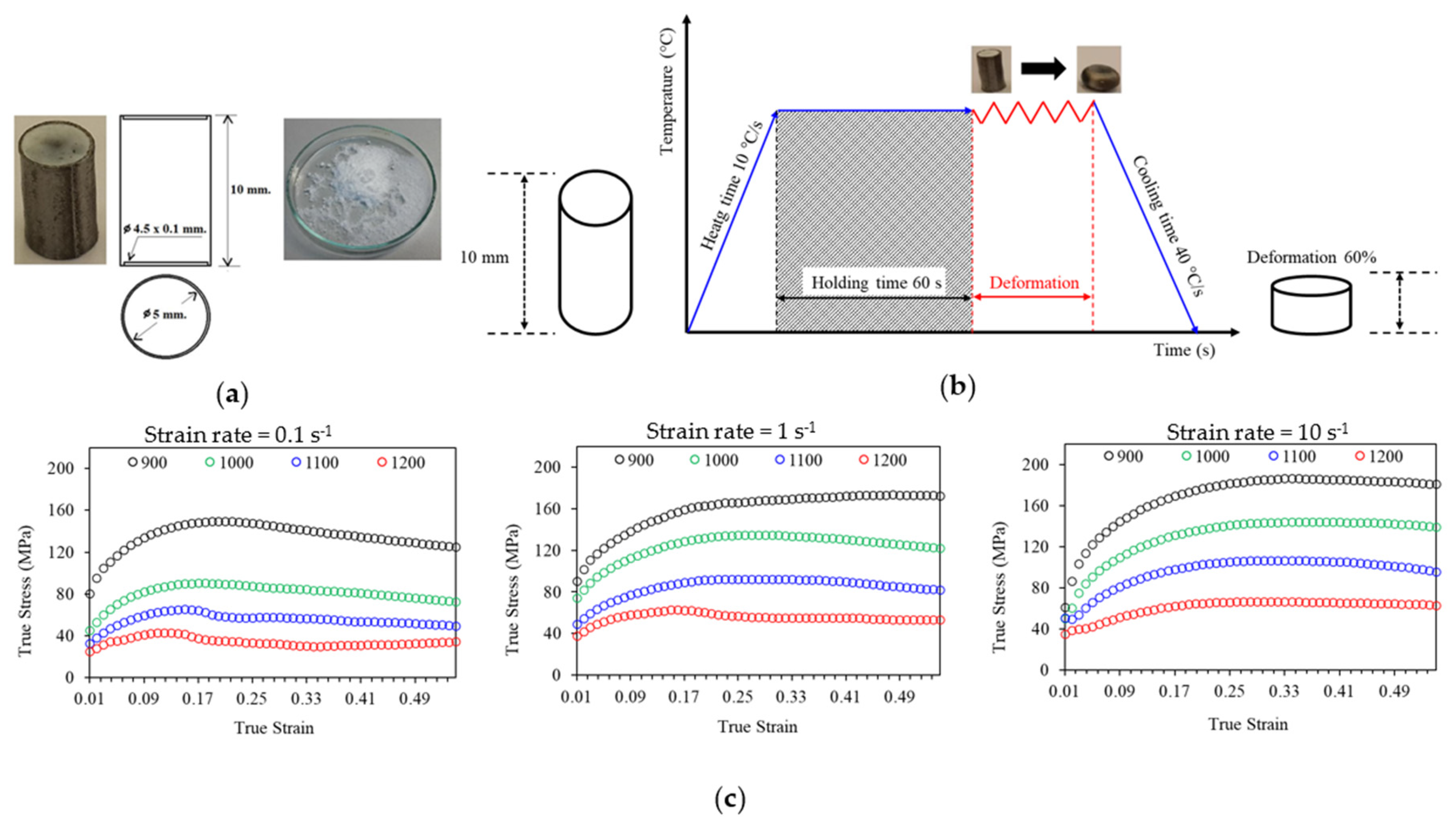
2.1. Materials

This study employed a material composition analysis and hot compression tests to evaluate the properties and performance of the materials under investigation.

Table 1. Chemical composition of the investigated AISI 1045 medium carbon steel (wt.%).

Element	C	Si	Mn	P	S	Cu	Cr	Ni	Mo	Fe
Nominal	0.42–0.48	0.15–0.35	0.60–0.90	Max. 0.03	Max. 0.035	Max. 0.3	Max. 0.2	Max. 0.2	-	Bal.
Actual	0.47	0.19	0.67	0.03	0.02	0.18	0.11	0.07	0.02	Bal.

displays the standard chemical composition of AISI 1045 carbon steel according to the AISI specifications [13], presented in weight percentage (wt.%). A chemical composition analysis of the materials was conducted using an emission spectrometer (manufacturer: Perkin Elmer; model: Optima 8000, Waltham, MA, USA) on two test specimens to validate these findings. The results in Table 1 reveal that the alloy steel contained elements such as carbon (C), nickel (Ni), chromium (Cr), and molybdenum (Mo). These elements contribute to its high strength, hardenability, and corrosion resistance. The similarity in chemical composition, particularly among the major constituents, confirmed the accurate comparison of the grade with AISI 1045 steel.

Hot compression tests were conducted using a deformation dilatometer (manufacturer: TA Instruments; model: DIL805, New Castle, DE, USA) with cylindrical samples (5 mm diameter, 10 mm height). A thermocouple measured the testing temperature directly. The tests were performed at four temperatures (900, 1000, 1100, and 1200 °C) and three strain rates (0.1, 1, and 10 s⁻¹). The samples were placed in a vacuum chamber filled with argon gas. They were heated by an induction coil at 1.625 °C/s to the test temperatures, held for 1 min, and then compressed to a 60% height reduction using an alumina powder, as shown in Figure 1a [14,15]. The samples were then quenched in argon gas at 40 °C/s to room temperature. Figure 1b shows the temperature–time route, and Figure 1c display the flow curves under various deformation conditions. The flow stress ($\sigma$) from the hot compression test, presented in terms of the strain ($\epsilon$), strain rate ($\dot{\epsilon }$), and temperature (T), was incorporated into the FEM simulation software (QForm V10.2.1).

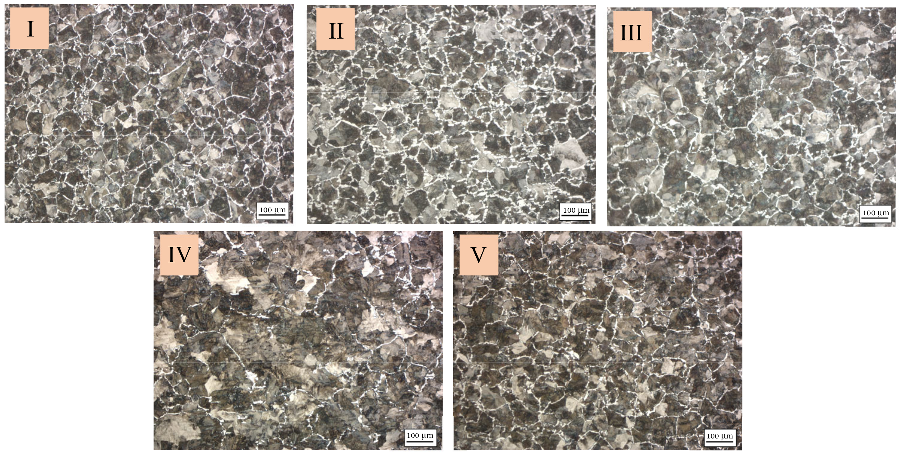
2.2. Microstructure Characterization

In this study, the verification of the FE simulation included the grain size and phase. Therefore, metallographic preparation was conducted on the samples. After mounting in a hot mounting press, the samples’ cutting surfaces were initially polished using 400-grit SiC abrasive paper. This was followed by polishing with 600, 800, 1000, and 1200 grit SiC papers, and finally, with 0.3 μm alumina particles. The polished surfaces were then etched using a 4% picral and 3% nital solution for 4 s. Microstructural observations were conducted using light optical microscopy (manufacturer: Carl Zeiss Microscopy; model: SteREO Discovery.V20, Jena, Germany).

2.3. Microstructure Evolution Model

During hot forging, dynamic recrystallization (DRX) plays a crucial role. This process, typically triggered by the accumulation of dislocations resulting from plastic deformation, leads to the formation of new, finer grains within the material [16,17]. To quantify this phenomenon, the Johnson–Mehl–Avrami–Kolmogorov (JMAK) microstructure model was employed [18,19,20]. This model, presented in Equation (1), enabled the calculation of the DRX volume fraction ($X_{\mathrm{d}}$) occurring within the material.

$$X_{\mathrm{d}}=1-\exp \left(-{\beta }_{\mathrm{d}}{\left({\displaystyle \frac{\epsilon -{\epsilon }_{\mathrm{c}}}{{\epsilon }_{0.5}}}\right)}^{k_{\mathrm{d}}}\right)$$

(1)

where coefficients ${\beta }_{\mathrm{d}}$ and $k_{\mathrm{d}}$ are the material constants, ${\epsilon }_{\mathrm{c}}$ is the critical strain for the initiation of DRX, and ${\epsilon }_{0.5}$ denotes the strain for achieving a 50% DRX volume fraction, as follows:

$${\epsilon }_{0.5}=A_{0.5}{d}_0^{M_{0.5}}{\dot{\epsilon }}^{L_{0.5}}\exp \left(Q_{0.5}/RT\right)$$

(2)

${\epsilon }_{\mathrm{c}}$ was determined using the approach by Poliak and Jonas [21], which suggested that identifying the inflection point in $\ln \theta -\epsilon$ plots indicates the initiation of DRX. This method helps determine the critical stress ${\sigma }_{\mathrm{c}}$ by pinpointing the inflection point. The corresponding ${\epsilon }_{\mathrm{c}}$ value can be derived through experimental stress–true strain curves. The relationship between the critical strain and the peak strain is given by ${\epsilon }_{\mathrm{c}}=\alpha {\epsilon }_{\mathrm{p}}$, where the peak strain, ${\epsilon }_{\mathrm{p}}$, denotes the strain value associated with the peak stress (${\sigma }_{\mathrm{p}}$). Taking into consideration the initial grain size ($d_0$), T, $\dot{\epsilon }$, and Q, one can formulate the expression for ${\epsilon }_{\mathrm{p}}$ as follows:

$${\epsilon }_{\mathrm{p}}=A_{\mathrm{p}}{d}_0^{M_{\mathrm{p}}}{\dot{\epsilon }}^{L_{\mathrm{p}}}\left(Q_{\mathrm{p}}/RT\right)$$

(3)

The average DRX grain size is defined as

$$D_{\mathrm{d}}=A_{\mathrm{d}}{d}_0^{M_{\mathrm{d}}}{\dot{\epsilon }}^{L_{\mathrm{d}}}\left(Q_{\mathrm{d}}/RT\right)$$

(4)

In this study, compression tests determined the coefficients for the microstructure evolution equations (Equations (1)–(4)) specific to AISI 1045 medium carbon steel, as shown in

Table 2. Coefficients in microstructure equations for the investigated steels.

${\mathit{A}}_{\mathbf{p}}$	${\mathit{M}}_{\mathbf{p}}={\mathit{M}}_{\mathbf{d}}={\mathit{M}}_{0.5}$	${\mathit{L}}_{\mathbf{p}}$	${\mathit{Q}}_{\mathbf{p}}$	α	${\mathit{A}}_{0.5}$	${\mathit{Q}}_{0.5}$	${\mathit{L}}_{0.5}$	${\mathit{k}}_{\mathbf{d}}$	${\mathit{\beta }}_{\mathbf{d}}$	${\mathit{Q}}_{\mathbf{d}}$	${\mathit{L}}_{\mathbf{d}}$	${\mathit{A}}_{\mathbf{d}}$
0.012	0	0.189	29,448.700	0.478	0.040	22,058.400	0.117	5.070	2.404	−67,793.200	−0.073	7082.570

, with reference to Siripath et al. [22]. An FE model incorporating these equations was implemented in FE software to predict the microstructure evolution of the forged components, particularly ball joints.

2.4. Design of Experiment

The Taguchi method, a widely used parameter design approach, is essential for robust design across industries and minimizes the number of experiments required by understanding the effects of different design parameters and optimizing their combination to reduce the sensitivity to external noise. This method utilizes orthogonal arrays (OAs) for experimental runs and signal-to-noise (SN) ratios to assess the performance quality. Higher S/N ratios indicate a better-quality performance, with noise representing variance. The S/N ratio is categorized into “lower is better” (LB), “nominal is best” (NB), and “higher is better” (HB) [23,24,25,26]. The S/N ratio of the ball joint process was chosen as LB, and it is as follows:

$${\displaystyle \frac{S}{N}}=-10\log {\displaystyle \frac{{\displaystyle \sum y^2}}{n}}$$

(5)

where n represents the number of experiments under identical design parameter conditions, y denotes the experimental results, and the subscript i corresponds to the number of design parameters in the OA table. For the forging investigation, three key process parameters were identified as control factors: the initial billet temperature, the billet length, and the coefficient of friction, as detailed in

Table 3. Simulation control factors and their different levels.

Factor	Units	Symbol	Level 1	Level 2	Level 3
Forging Temperature	°C	A	1000	1100	1200
Billet Size	mm	B	230	240	250
Friction Factor	-	C	0.15	0.50	0.64

. The friction factor was determined by lubricant type with a ring compression test [27]. To efficiently design a set of nine FE simulations, an orthogonal array (OA) approach was adopted, specifically an L9 array. The MINITAB (manufacturer: Minitab Pty Ltd.; model: Minitab 17, State College, PA, USA) software was used to analyze the generated data.

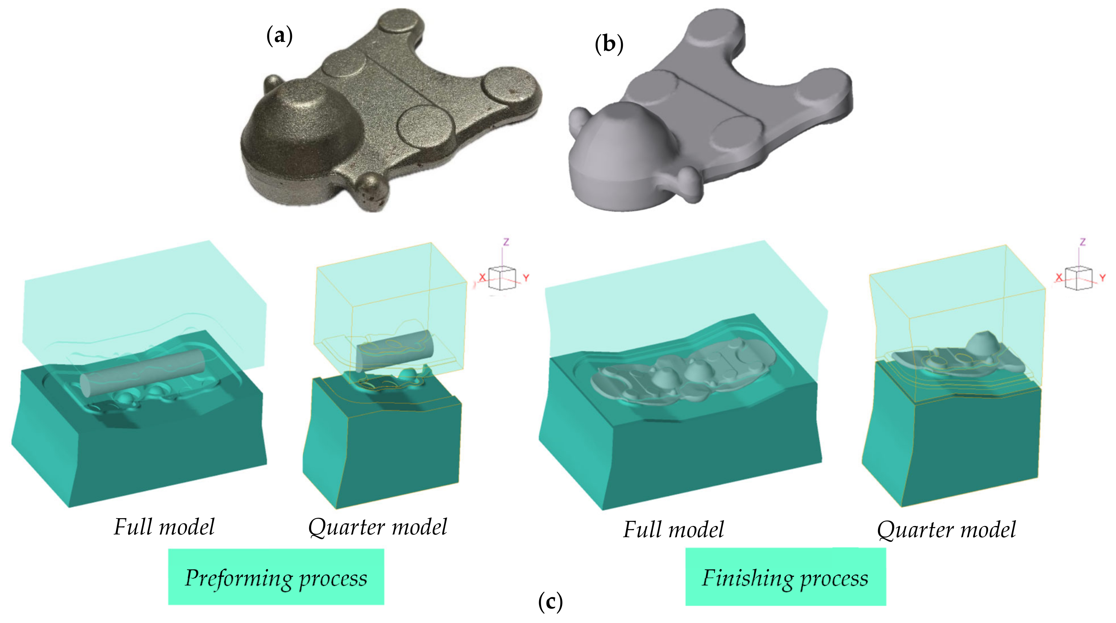
2.5. FE Simulation of Ball Joint

The ball joint was produced through the hot forging process, which comprised three primary stages: preforming, finishing, and flash trimming. Following the finishing stage of forging, excess flash was removed, and the workpiece was cooled to ambient temperature. The preforming die surface was more profound than the finishing die surface by about 1 mm. Figure 2 depicts the 3D-CAD model alongside the actual workpiece and FE model of the complete hot forging process for the ball joint. For this simulation, a quarter symmetry model was utilized. The billet was modeled with plastic behavior, whereas the upper and lower dies were defined as rigid bodies. The friction factor between the die and the workpiece was kept constant throughout. The simulation parameters were set according to the specific conditions of the hot forging process for the ball joint, as detailed in

Table 4. The operation parameters assigned to complete the simulation.

Parameter	Description
Element type	Tetrahedral
Number of nodes: initial billet	800
Number of surface elements: initial billet	1180
Number of volumetric elements: initial billet	2944
Die’s temperature	250 °C
Forging equipment	Crank press JFP-1350 M/C (Gyeonggi-do, Republic of Korea)
Strokes per minute	85
Stroke length	240
Crank radius to conrod length ratio	0.15

.

3. Results

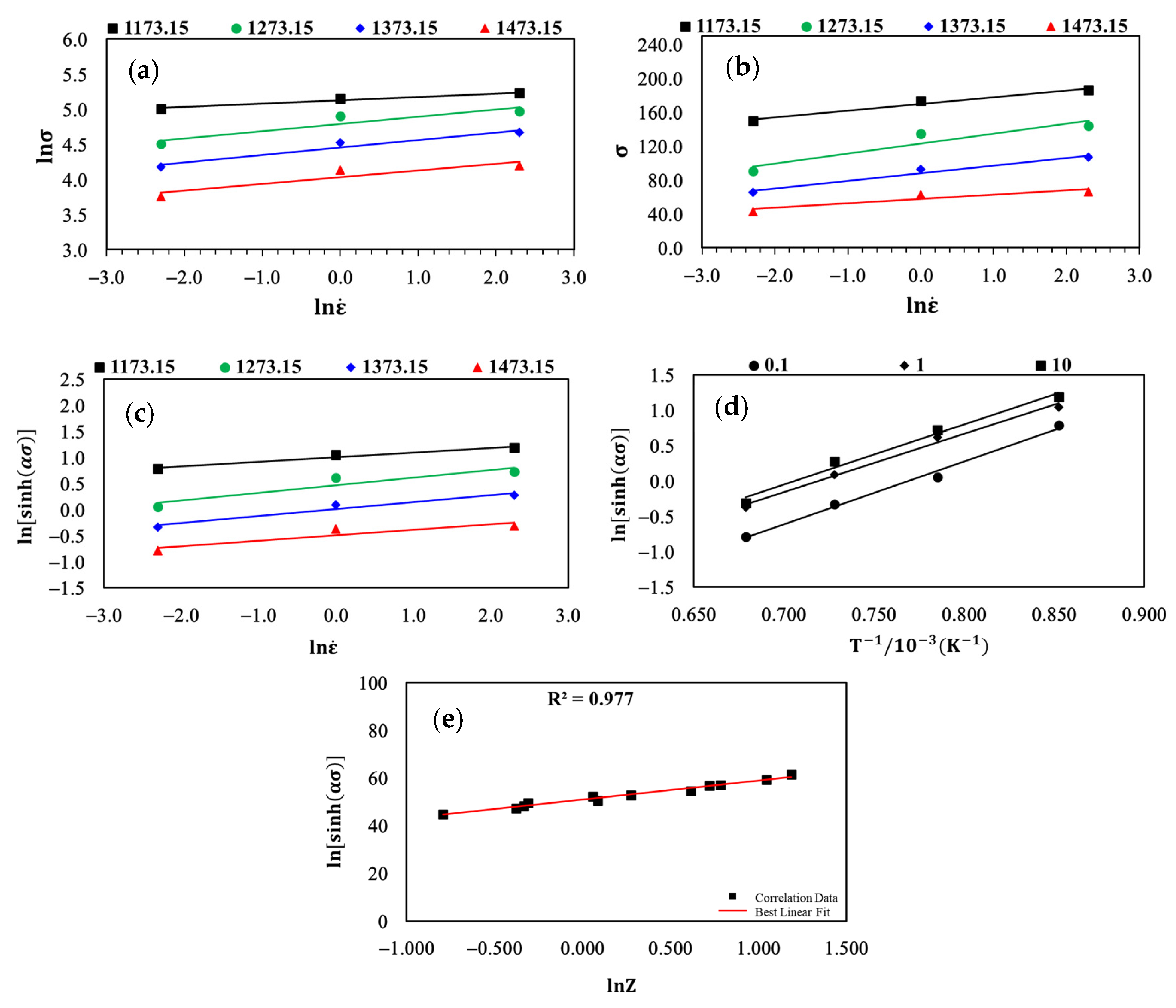
3.1. Modeling the Arrhenius-Based Constitutive Equation

The Zener–Hollomon parameter (Z) relates the strain rate ($\dot{\epsilon }$) and temperature (T) during plastic deformation, as shown in Equation (6) [28]. According to Sellars and McTegart [29], they introduced the Arrhenius constitutive model (Equation (7)), which accurately depicts the relationship between the flow stress, strain rate, and deformation temperature. This model is particularly valuable for understanding materials’ flow behavior at temperatures above their recrystallization points, where significant changes in mechanical properties occur and deformation mechanisms become more complex [30,31].

$$Z=\dot{\epsilon }\exp \left(Q/RT\right)$$

(6)

$$\dot{\epsilon }=Af(\sigma )\exp \left(-Q/RT\right)$$

(7)

where

$$f(\sigma )=\left\{\begin{array}{c}\alpha {\sigma }^{n^{\prime }}\\ \exp (\beta \sigma )\\ {\left[\sinh (\alpha \sigma )\right]}^n\end{array}\right.\begin{array}{c}: \alpha \sigma <0.8\\ : \alpha \sigma >1.2\\ : \mathrm{for} \mathrm{all} \sigma \end{array}$$

(8)

In these equations, A represents a material-specific constant associated with the speed of dislocation movement within the crystal lattice. Q denotes the activation energy for deformation (kJ/mol), which is a characteristic property of the material. R is the universal gas constant (8.314 J/mol·K), T stands for the absolute temperature (K), σ represents the applied stress on the material (MPa), and n is the strain rate sensitivity exponent. This exponent indicates how the material’s deformation rate changes in response to variations in stress and temperature.

To determine the material constants for the Zener–Hollomon equation, the following relations were derived from the peak stress [32,33]. The values for n′ and β were obtained by substituting Equation (8) into Equation (7) at lower stress levels (ασ < 0.8) and higher stress levels (ασ > 1.2), respectively. The natural logarithm was subsequently applied to both sides of each equation, resulting in the following expressions:

$$\ln \dot{\epsilon }=n^{\prime }\ln \sigma +\ln A-Q/RT$$

(9)

$$\ln \dot{\epsilon }=\beta \sigma +\ln A-\left(Q/RT\right)$$

(10)

For a constant temperature and with the activation energy considered fixed, differentiating Equation (9) and Equation (10), respectively, yielded the following:

$${\left[{\displaystyle \frac{\partial \ln \dot{\epsilon }}{\partial \ln \sigma }}\right]}_T=n^{\prime }$$

(11)

$${\left[{\displaystyle \frac{\partial \ln \dot{\epsilon }}{\partial \sigma }}\right]}_T=\beta$$

(12)

The material constants can be found through the linear regression method. The values of n’ and β can be obtained from the slopes of the fitting lines presented in the plots of $\ln \dot{\epsilon }-\ln \sigma$ and $\ln \dot{\epsilon }-\sigma$. As illustrated in Figure 3a,b, the Q values were obtained by substituting Equation (8) with Equation (7) across all stress levels. Subsequently, the natural logarithm was applied to both sides of each equation, resulting in Equation (13).

$$\ln \dot{\epsilon }=\ln A+n\ln [\sinh (\alpha {\sigma }_{\mathrm{p}})]-\left(Q/RT\right)$$

(13)

By the partial differentiation of Equation (13), the apparent activation energy Q under a high temperature can be expressed:

$$Q=R{\left[{\displaystyle \frac{\partial \ln (\dot{\epsilon })}{\partial \ln [\sinh (\alpha \sigma )]}}\right]}_{\mathrm{T}}{\left[{\displaystyle \frac{\partial \ln [\sinh (\alpha \sigma )]}{\partial (1/T)}}\right]}_{\dot{\epsilon }}$$

(14)

As per Equation (9), Q was calculated based on the slopes observed in the scatter plots of $\ln \left[\sinh (\alpha \sigma )\right]-\ln \dot{\epsilon }$ and $\ln \left[\sinh (\alpha \sigma )\right]-1/T$ in Figure 3c and Figure 3d, respectively. By utilizing Equations (6)–(8), as depicted in Equation (15), the relationship between the Z parameter and the true stress can be established. Furthermore, the natural logarithm was subsequently applied to both sides of Equation (13) to yield a modified equation, expressed as Equation (16):

$$Z=\dot{\epsilon }\exp \left(Q/RT\right)=A{\left[\sinh (\alpha \sigma )\right]}^n$$

(15)

$$\ln Z=\ln A+n\ln \left[\sinh (\alpha \sigma )\right]$$

(16)

The scatter plot of $\ln Z-\ln \left[\sinh (\alpha \sigma )\right]$ displayed in Figure 3e demonstrates a good linear correlation, indicating a good fit. The intercept and slope of this plot correspond to the values of A and n. The material constants for the Arrhenius-based constitutive model are presented in

Table 5. Material constant for the general expression of the Arrhenius-based constitutive model derived from the peak stress.

n′	β	α	n	Q	$\mathbf{ln}\mathit{A}$	A
11.60611	0.11840	0.01020	8.12972	577.20710	50.87365	1.2421 × 1022

.

The Zener–Hollomon parameter in Equation (17) represents the flow stress. The predicted flow curve can be obtained by substituting the material constants corresponding to each deformation condition. The predicted flow curve was compared with the experimental data, as illustrated in Figure 4. The prediction accuracy was evaluated by analyzing the correlation coefficient (R²) and the average absolute relative error (AARE) [34,35]. The results show that the prediction model was highly accurate, with an R² value of 0.968 and an AARE of 7.079% The developed constitutive models, based on the Arrhenius equation, were implemented into finite element software to optimize the process conditions for manufacturing the ball joint.

$$\sigma ={\displaystyle \frac{1}{\alpha }}\ln {\left\{{\left({\displaystyle \frac{Z}{A}}\right)}^{1/n}+\left[{\left({\displaystyle \frac{Z}{A}}\right)}^{2/n}+1\right]\right\}}^{1/2}$$

(17)

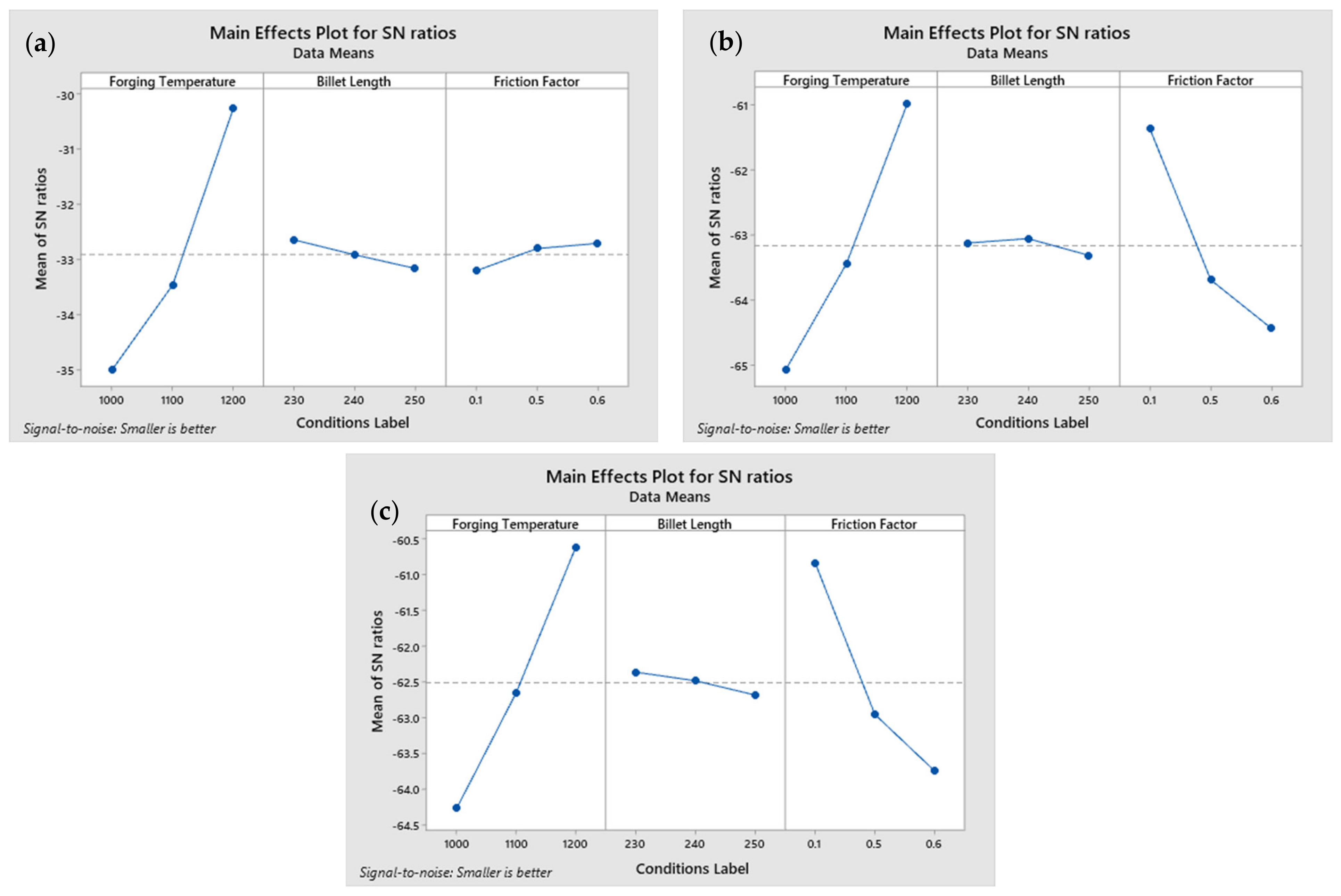
3.2. S/N Ratio Analysis

In the Taguchi method, FE simulations were employed to investigate three key parameters: the friction factor, the length of the billet, and the billet temperature. These parameters were optimized to improve the forging conditions.

Table 6. L9 orthogonal design array and their simulation result for the forging load (tf) and maximum mean stress (MPa).

Exp. No.	A (°C)	B (mm)	C	Max. Preforming Force (tf)	Max. Finishing Force (tf)	Max. Mean Stress (MPa)	S/N Ratios
							Max. Preforming Force	Max. Finishing Force	Max. Mean Stress
1	1000	230	0.100	1444.000	1321.000	60.125	−63.191	−62.418	−35.581
2	1000	240	0.500	1912.000	1732.000	53.994	−65.630	−64.771	−34.647
3	1000	250	0.600	2093.000	1916.000	54.965	−66.415	−65.648	−34.802
4	1100	230	0.500	1556.000	1398.000	43.801	−63.840	−62.910	−32.830
5	1100	240	0.600	1691.000	1554.000	49.026	−64.563	−63.829	−33.809
6	1100	250	0.100	1248.000	1151.000	48.716	−61.924	−61.222	−33.754
7	1200	230	0.600	1310.000	1226.000	29.927	−62.345	−61.770	−29.521
8	1200	240	0.100	889.000	877.000	32.704	−58.978	−58.860	−30.292
9	1200	250	0.500	1203.000	1147.000	35.229	−61.605	−61.191	−30.938

presents the recorded values of the forging load, the mean tensile stress for the simulation process, and their corresponding calculated S/N ratios. Higher S/N ratios indicated a better quality, emphasizing the importance of optimizing parameters with superior S/N ratios in the Taguchi analysis. Specifically, achieving a ”smaller-is-better” S/N ratio for a lower forging load indicates less energy consumption and potentially less wear on equipment, contributing to more efficient and sustainable manufacturing processes. Similarly, minimizing the S/N ratio for the maximum mean stress ensures the greater structural integrity and reliability of the forged components, which is crucial for meeting stringent performance standards in various applications.

Table 7. S/N response table for force and maximum mean stress.

Levels	Control Factors
	Maximum Preforming Force (tf)			Maximum Finishing Force (tf)			Maximum Mean Stress (MPa)
	A	B	C	A	B	C	A	B	C
1	−65.08	−63.13	−61.36	−64.28	−62.37	−60.83	−35.01	−32.64	−33.21
2	−63.44	−63.06	−63.69	−62.65	−62.49	−62.96	−33.46	−32.92	−32.80
3	−60.98	−63.31	−64.44	−60.61	−62.69	−63.75	−30.25	−33.16	−32.71
Delta	4.10	0.26	3.08	3.67	0.32	2.92	4.76	0.52	0.50
Rank	1	3	2	1	3	2	1	2	3

The S/N response values marked in bold indicate different significance levels and influences for each variable.

presents the S/N responses for the maximum stress and force, revealing the optimal levels of the control factors influencing these parameters. These results are visually depicted in Figure 5. Based on these findings, the optimal conditions for forging the ball joint were determined to be a billet temperature of 1200 °C, a billet length of 230 mm, and a friction factor of 0.1, which yielded the highest S/N ratio, referring to the scenario where the strength of the desired signal is maximized relative to the background noise. In technical and analytical contexts, the highest S/N ratio indicates that the signal of interest is most prominent and least affected by noise or interference, resulting in more precise, more reliable data or output. A higher S/N ratio generally signifies a better performance or more accurate results in processes such as experimental testing. However, the S/N ratio for the maximum preforming load and maximum mean stress indicates potential data discrepancies or suggests the necessity for further investigation within the tested range. Conducting an analysis of variance (ANOVA) would help to determine the significance of these factors and identify any underlying patterns or inconsistencies that need to be addressed [12].

3.3. Analysis of Variance (ANOVA)

As seen in

Table 8. ANOVA table for maximum forging forces and mean stresses.

Factor	DOF	Sum of Squares	Mean Squares	% Contribution	F-Value	p-Value
Maximum preforming force
A	2	699,442.000	349,721.000	62.30%	101.450	0.010
B	2	10,065.000	5032.000	0.90%	1.460	0.407
C	2	406,244.000	203,122.000	36.19%	58.930	0.017
Error	2	6894.000	3447.000	0.61%
Total	8	1,122,645.000		100.00%
Maximum finishing force
A	2	492,503.000	246,251.000	59.50%	103.430	0.010
B	2	13,610.000	6805.000	1.64%	2.860	0.259
C	2	316,795.000	158,397.000	38.28%	66.530	0.015
Error	2	4762.000	2381.000	0.58%
Total	8	827,669.000		100.00%
Maximum mean stress
A	2	859.930	429.965	94.20%	25.300	0.038
B	2	4.360	2.180	0.48%	0.130	0.886
C	2	14.621	7.310	1.60%	0.430	0.699
Error	2	33.991	16.995	3.72%
Total	8	912.901		100.00%

, the analysis provided significant insights into the factors influencing the experimental outcomes in the Taguchi method study across the maximum preforming force, maximum finishing force, and maximum mean stress. The billet temperature emerged as highly influential across all measures, contributing substantially with percentages of 62.30% for the preforming force, 59.50% for the finishing force, and 94.20% for the mean stress. It demonstrated a strong effect with its respective F-values and p-values (preforming force: p = 0.01, F = 101.45; finishing force: p = 0.01, F = 103.43; mean stress: p = 0.038, F = 25.3), highlighting its pivotal role in shaping the response variables. In contrast, the billet size showed minimal influence across all measures, with non-significant effects and marginal contributions (preforming force: p = 0.407, F = 1.46, 0.90%; finishing force: p = 0.259, F = 1.64, 1.64%; mean stress: p = 0.886, F = 0.13, 0.48%). The friction factor also displayed notable effects on the preforming force (p = 0.017, F = 58.93, 36.19%) and finishing force (p = 0.015, F = 66.53, 38.28%), contributing significantly to the outcome variability. However, it showed minimal influence on the mean stress (p = 0.699, F = 0.43, 1.60%). The error term was consistently minimal across all measures (preforming force: 0.61%, finishing force: 0.61%, mean stress: 3.72%), indicating the effective capture of the observed variability. These findings underscore the critical importance of optimizing the billet temperature and friction factor settings to enhance the quality and efficiency of the forging process, while suggesting that adjustments to the billet size and friction factor may have a limited practical impact in this specific context.

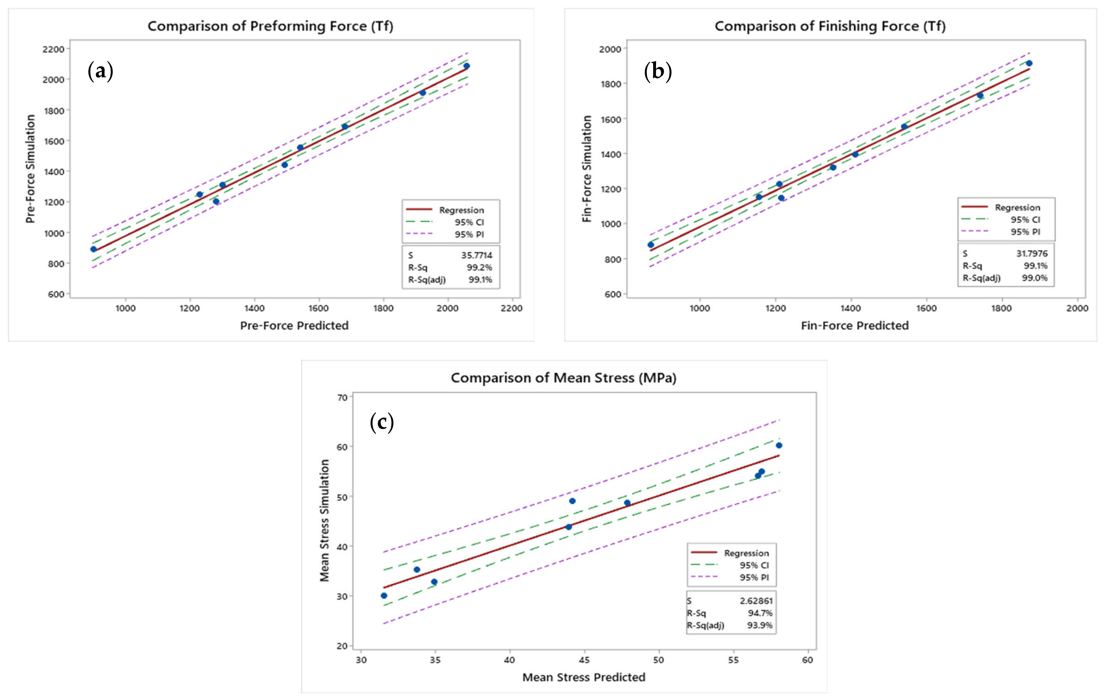
3.4. Regression Analysis

This study conducted regression analyses to explore the relationships between various dependent and independent variables. The dependent variables examined were the maximum preforming forces, maximum finishing forces, and maximum mean stress. The independent variables included the forging temperature (A), billet size (B), and friction factor (C) at the die and workpiece interface. The results of the linear regression analysis yielded predictive equations for the dependent variables, which are presented below.

Maximum preforming force (tf) = 3908 − 3.412A + 3.90B + 980.0C

(18)

Maximum finishing force (tf) = 3100 − 2.865A + 4.48B + 862.4C

(19)

Maximum mean stress (MPa) = 158.0 − 0.1187A + 0.084B − 5.66C

(20)

Additionally, plots comparing the predicted and simulated values of the maximum preforming forces, maximum finishing forces, and maximum mean stress are shown in Figure 6. The R² values for each regression analysis were 0.992, 0.991, and 0.947, respectively. The results demonstrate that the R² values are close to 1, indicating a strong correlation between the predicted and simulated values and confirming the reliability and accuracy of the regression model. The green dashed line represents the 95% confidence interval (CI), indicating the precision of the regression predictions. Meanwhile, the purple dashed line depicts the 95% prediction interval (PI), showing the range within which future observations are likely to fall. These intervals further underscore the robustness of the regression model in estimating the maximum preforming forces, maximum finishing forces, and maximum mean stress based on the independent variables studied.

3.5. Verification Results of FEM

Following the regression analysis, the verification results using the finite element method (FEM) were examined. Employing the Taguchi method, the optimal parameters for forging AISI 1045 medium carbon steel ball joints were determined based on three key responses: the maximum preforming forces, the maximum finishing forces, and the maximum mean stress. The optimal process parameters identified included an initial temperature of 1200 °C, a billet length of 230 mm, and a friction factor of 0.1. These parameters were validated through simulation software and practical shop floor experiments to ensure accurate ball joint production in conjunction with the predictive regression models. A post-experiment analysis showed that the produced parts were free of defects and exhibited complete filling, confirming the effectiveness and reliability of the optimized parameters.

Table 9. Forging forces from the predictive regression model and FE simulation, with percent errors compared to actual experiments.

Forging Force	Experiment	Predictive Model	FE Simulation	%Error (Predictive Model)	%Error (FE Simulation)
Preforming force (tf)	1044.70	857.60	1074.80	17.9094	2.8812
Finishing force (tf)	980.60	821.70	1013.90	16.2043	3.3959

presents the forging forces from the predictive regression model, the FE simulation, and their percent errors compared to the actual experiments. The results compared the predictive regression model, FE simulation, and experimental data for the forging forces while producing AISI 1045 medium carbon steel ball joints. For the preforming force, the predictive model estimated 857.60 tf, while the FE simulation predicted 1074.8 tf. This resulted in percentage errors of 17.9094% for the predictive model and 2.8812% for the FE simulation, indicating a slightly higher discrepancy in the predictive model’s estimation. Similarly, for the finishing force, the predictive model and FE simulation predicted 821.70 tf and 1013.9 tf, respectively, with percentage errors of 16.2043% and 3.3959%. These results suggest that, while the predictive model and FE simulation provided reasonably accurate estimations, the FE simulation tended to be closer to the experimental results for both forging forces. Overall, the observed discrepancies highlight the importance of using both predictive modeling and an FE simulation with practical experiments to optimize the process parameters effectively and ensure the production of defect-free ball joints.

In this study, the FE simulation results, depicted in Figure 7, provide a comprehensive visualization of the forging process, including the distance to contact, the plastic strain, the effective stress, and the temperature distribution after the preforming and finishing stages. Figure 7a shows the distance to contact, with the contour colors representing the spacing between the tools and the workpiece surface, measured perpendicular to the forging die. Figure 7b illustrates the plastic deformation distribution through a contour color plot of the plastic strain, highlighting the regions of significant deformation that indicate potential failure zones and high-stress concentrations, which are crucial for understanding material behavior under complex loading and improving the component design. Figure 7c reveals the effective stress concentration along the flank edge of the workpiece near the flash region, with a noticeable increase during the finishing process due to higher forming loads. Figure 7d displays the temperature distributions post-forging, starting from an initial 1200 °C, with high temperatures on the workpiece surface and within, resulting from the conversion of plastic deformation into heat. The prolonged contact with the die caused a temperature drop due to heat transfer, while the flash area consistently showed higher temperatures at the end of each operation due to increased deformation and die friction. These visualizations collectively offer valuable insights into material behavior and the forging process, aiding in making informed decisions to enhance the design and prevent component failure.

The simulation of the forging process for manufacturing a ball joint utilized a microstructure evolution model with coefficients specifically tailored for AISI 1045 medium carbon steel, as developed by Siripath, Suranuntchai, and Sucharitpwatskul [22]. Figure 8 illustrates the forged ball joint, highlighting the distribution of the grain size (μm), tensile strength (MPa), and pearlite volume fraction (%) through contour colors. The FE simulation results indicated that the grain sizes within the forged component ranged from 6.762 μm to 45.405 μm. A cross-section of the ball joint, prepared for microstructural examination, is shown in Figure 9, with five marked investigation points. Figure 10 displays the distribution of the grain size, pearlite volume fraction, and ferrite volume fraction at these cross-sections, as determined by the FE simulation. To validate the simulation, the actual grain sizes were obtained through a metallographic image analysis, as shown in Figure 11. The analysis revealed an average grain size of 36.982 μm across the five points. A bar graph in Figure 12a compares the measured and simulated grain sizes at each point. This comparison revealed an average error of 15.159%, with the errors ranging from 8.007% to 19.465%. The error distribution’s standard deviation of 5.910 μm suggests consistent deviations between the simulated and measured grain sizes. This indicates that, while the simulation provided a reasonably accurate prediction of the grain size distribution, some discrepancies could be attributed to factors such as model limitations or variations in the actual forging process. Overall, the simulation’s ability to closely approximate the real measurements demonstrates its usefulness in predicting the microstructural outcomes in forged components.

In addition to the final structure of a forged ball joint being significantly influenced by the material transformations occurring during cooling, this study employed FE simulation software that integrated the built-in material library to predict these transformations accurately. After the forging process, the ball joint undergoes natural cooling, resulting in a microstructure consisting of proeutectoid ferrite and pearlite, as confirmed by the microstructure analysis presented in Figure 11. This transformation is consistent with the continuous cooling transformation (CCT) diagram predictions for the material used. The predicted pearlite volume fraction within the forged component was compared to actual measurements to validate the FE simulation’s accuracy. Figure 10b displays the simulation results, while the bar graph in Figure 12b presents the measured volume fraction data. The model demonstrated a remarkable accuracy in predicting the pearlite volume fraction at all five designated study points, with a minimal error of only 7.3016%.

4. Conclusions

This study investigated the application of the Taguchi method and an FE simulation to optimize the hot forging process for AISI 1045 medium carbon steel ball joints. The key findings are as follows:

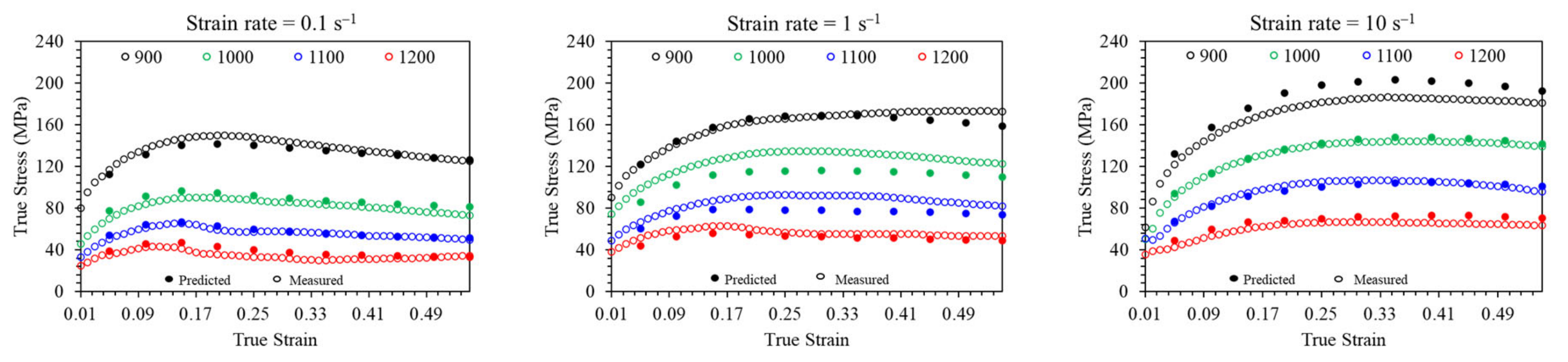
• The Arrhenius constitutive model accurately predicted the flow stress under various strain rates and temperatures based on the Zener–Hollomon parameter. With an R² of 0.968 and an AARE of 7.079, the model showed a high precision in its predictions. These constants have effectively optimized the manufacturing processes for AISI 1045 ball joints. Integrating these models into finite element software has proven valuable for improving process conditions.
• The Taguchi method and FE simulations identified the optimal forging parameters—a billet temperature of 1200 °C, a billet length of 230 mm, and a friction factor of 0.1. The ANOVA showed that the billet temperature significantly affected the preforming force (62.30%), finishing force (59.50%), and mean stress (94.20%), while the friction factor impacted the preforming (36.19%) and finishing forces (38.28%). The regression analyses, with high R² values, validated the predictive accuracy of these parameters. Overall, the billet temperature and friction factor were crucial for optimizing the forging efficiency, with less impact from the billet size.
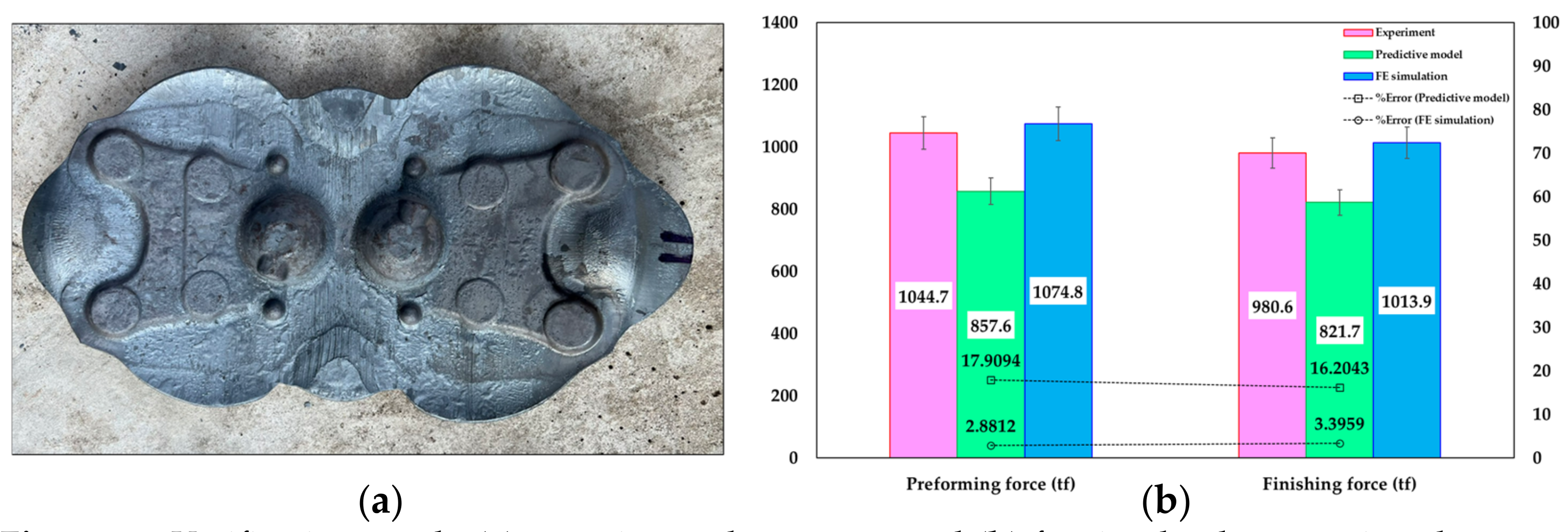
• Verifying the optimal forging parameters through a simulation and practical experiments confirmed the effectiveness of these parameters, resulting in defect-free components and accurate production outcomes in Figure 13a. The FE simulation showed minimal discrepancies in the forging forces compared to predictive models, with percentage errors of 2.88% for the preforming force and 3.40% for the finishing force, indicating a high accuracy (Figure 13b). Additionally, the FE simulation visualizations provided insights into the stress distribution and temperature changes, enhancing the understanding and design of the forging process.
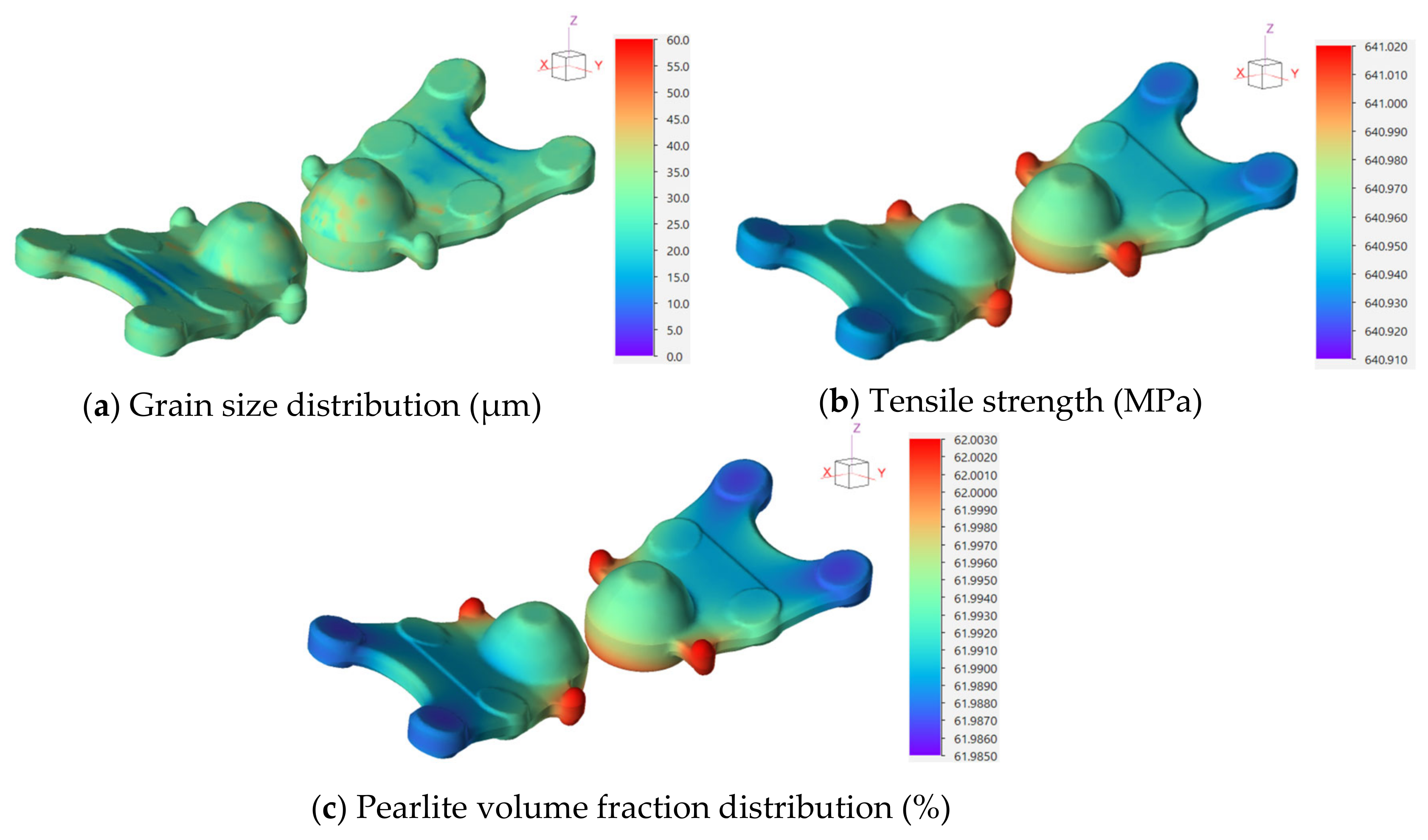
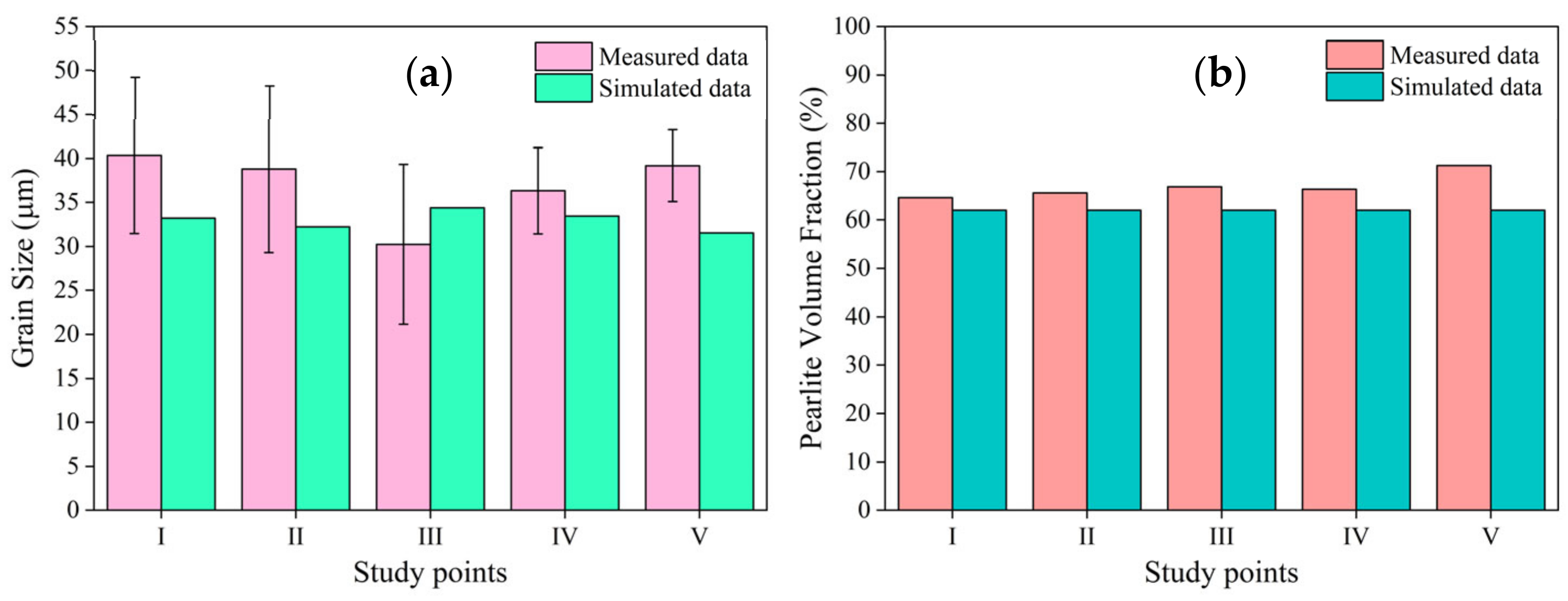
• The study also investigated microstructure evolution modeling to predict the grain size distribution and microstructural changes in AISI 1045 medium carbon steel post-forging. The FE simulations estimated grain sizes between 6.762 μm and 45.405 μm, with the actual measurements revealing an average grain size of 36.982 μm and an average error of 15.159% compared to the simulations. The model accurately predicted the pearlite volume fraction, with a minimal error of 7.3016%, confirming its effectiveness in forecasting the key microstructural outcomes in forged components.

References

1. Altan, T. Cold and Hot Forging: Fundamentals and Applications; Gracious Ngaile, G.S., Ed.; ASM International: Materials Park, OH, USA, 2005; p. 341. [Google Scholar]
2. Huang, S.-Q.; Yi, Y.-P.; Zhang, Y.-X. Simulation of 7050 Wrought Aluminum Alloy Wheel Die Forging and its Defects Analysis based on DEFORM. In Proceedings of the AIP Conference Proceedings, Pohang, Republic of Korea, 15 June 2010; pp. 638–644. [Google Scholar]
3. Bonte, M.H.A.; Fourment, L.; Do, T.-T.; van den Boogaard, A.H.; Huétink, J. Optimization of forging processes using Finite Element simulations. Struct. Multidiscipl. Optim. 2010, 42, 797–810. [Google Scholar] [CrossRef]
4. Sukjantha, V.; Aue-u-lan, Y. Determination of Optimal Preform Part for Hot Forging Process of the Manufacture Axle Shaft by Finite Element Method. Appl. Sci. Eng. Prog. 2013, 6, 35–42. [Google Scholar]
5. Tenesgen, A.D.; Irfaan, M.; Bhardwaj, B. Improvement of Hot Forging Process by Minimized Die Stress using Finite Element Method. Int. J. Eng. Sci. Technol. 2015, 3, 1316–1329. [Google Scholar]
6. Pundir, R.; Chary, G.H.V.C.; Dastidar, M.G. Application of Taguchi method for optimizing the process parameters for the removal of copper and nickel by growing Aspergillus sp. Water Resour. Ind. 2018, 20, 83–92. [Google Scholar] [CrossRef]
7. Kivak, T.; Samtaş, G.; Çiçek, A. Taguchi method based optimisation of drilling parameters in drilling of AISI 316 steel with PVD monolayer and multilayer coated HSS drills. Measurement 2012, 45, 1547–1557. [Google Scholar] [CrossRef]
8. Chen, X.; Jung, D. Gear hot forging process robust design based on finite element method. J. Mech. Sci. Technol. 2008, 22, 1772–1778. [Google Scholar] [CrossRef]
9. Choi, S.K.; Chun, M.S.; Van Tyne, C.J.; Moon, Y.H. Optimization of open die forging of round shapes using FEM analysis. J. Mater. Process. Technol. 2006, 172, 88–95. [Google Scholar] [CrossRef]
10. Equbal, I.; Ohdar, R.; Bhat, N.S.; Ahmad, S. Preform Shape Optimization of Connecting Rod Using Finite Element Method and Taguchi Method. Int. J. Mod. Eng. Res. 2012, 2, 4532–4539. [Google Scholar]
11. Sanjari, M.; Taheri, A.K.; Movahedi, M.R. An optimization method for radial forging process using ANN and Taguchi method. Int. J. Adv. Manuf. Technol. 2009, 40, 776–784. [Google Scholar] [CrossRef]
12. Obiko, J.O.; Mwema, F.M.; Shangwira, H. Forging optimisation process using numerical simulation and Taguchi method. SN Appl. Sci. 2020, 2, 713. [Google Scholar] [CrossRef]
13. Riaz, M.; Atiqah, N. A Study on the Mechanical Properties of S45c Medium Type Carbon Steel Specimens under Lathe Machining and Quenching Conditions. Int. J. Res. Eng. Technol. 2014, 3, 121–130. [Google Scholar]
14. Gutierrez-Gonzalez, C.F.; Smirnov, A.; Centeno, A.; Fernández, A.; Alonso, B.; Rocha, V.G.; Torrecillas, R.; Zurutuza, A.; Bartolome, J.F. Wear behavior of graphene/alumina composite. Ceram. Int. 2015, 41, 7434–7438. [Google Scholar] [CrossRef]
15. Gutiérrez-Mora, F.; Cano-Crespo, R.; Rincón, A.; Moreno, R.; Domínguez-Rodríguez, A. Friction and wear behavior of alumina-based graphene and CNFs composites. J. Eur. Ceram. Soc. 2017, 37, 3805–3812. [Google Scholar] [CrossRef]
16. Bharath, K.; Khanra, A.K.; Davidson, M. Hot deformation behavior and dynamic recrystallization constitutive modeling of Al–Cu–Mg powder compacts processed by extrusion at elevated temperatures. Proc. Inst. Mech. Eng. Part L J. Mater. Des. Appl. 2021, 235, 581–596. [Google Scholar] [CrossRef]
17. Sakai, T.; Belyakov, A.; Kaibyshev, R.; Miura, H.; Jonas, J.J. Dynamic and post-dynamic recrystallization under hot, cold and severe plastic deformation conditions. Prog. Mater. Sci. 2014, 60, 130–207. [Google Scholar] [CrossRef]
18. Irani, M.; Lim, S.; Joun, M. Experimental and numerical study on the temperature sensitivity of the dynamic recrystallization activation energy and strain rate exponent in the JMAK model. J. Mater. Res. Technol. 2019, 8, 1616–1627. [Google Scholar] [CrossRef]
19. Quan, G.-z.; Shi, R.-j.; Zhao, J.; Liu, Q.; Xiong, W.; Qiu, H.-m. Modeling of dynamic recrystallization volume fraction evolution for AlCu4SiMg alloy and its application in FEM. Trans. Nonferrous Met. Soc. China 2019, 29, 1138–1151. [Google Scholar] [CrossRef]
20. Ji, H.; Peng, Z.; Huang, X.; Wang, B.; Xiao, W.; Wang, S. Characterization of the Microstructures and Dynamic Recrystallization Behavior of Ti-6Al-4V Titanium Alloy through Experiments and Simulations. J. Mater. Eng. Perform. 2021, 30, 8257–8275. [Google Scholar] [CrossRef]
21. Poliak, E.; Jonas, J. Initiation of Dynamic Recrystallization in Constant Strain Rate Hot Deformation. ISIJ Int. 2003, 43, 684–691. [Google Scholar] [CrossRef]
22. Siripath, N.; Suranuntchai, S.; Sucharitpwatskul, S. Modeling Dynamic Recrystallization Kinetics in BS 080M46 Medium Carbon Steel: Experimental Verification and Finite Element Simulation. Int. J. Technol. 2024, 15, 1292–1307. [Google Scholar] [CrossRef]
23. Kumar, V.; Kumari, N. Modeling and multiple performance optimization of ultrasonic micro-hole machining of PCD using fuzzy logic and taguchi quality loss function. Adv. Mater. Res. 2012, 1, 129–146. [Google Scholar] [CrossRef]
24. Wu, D.; Chang, M. Use of Taguchi method to develop a robust design for the magnesium alloy die casting process. Mater. Sci. Eng. A-Struct. Mater. 2004, 379, 366–371. [Google Scholar] [CrossRef]
25. Phadke, M.S. Quality Engineering Using Robust Design; Prentice Hall: Upper Saddle River, NJ, USA, 1989. [Google Scholar]
26. Jamaluddin, H.; Ghani, J.A.; Deros, B.M.; Rahman, M.N.A.; Ramli, R.B. Quality improvement using Taguchi method in shot blasting process. J. Mech. Eng. Sci. 2016, 10, 2200–2213. [Google Scholar]
27. Poungprasert, R.; Siripath, N.; Suranuntchai, S. A Comparative Study of Lubrication Performance for Bs 080M46 Medium Carbon Steel Using Ring Compression Test and Finite Element Simulation. Key Eng. Mater. 2024, 973, 37–44. [Google Scholar] [CrossRef]
28. Lin, Y.-C.; Chen, M.-S.; Zhang, J. Modeling of flow stress of 42CrMo steel under hot compression. Mater. Sci. Eng. A 2009, 499, 88–92. [Google Scholar] [CrossRef]
29. Sellars, C.M.; McTegart, W.J. On the mechanism of hot deformation. Acta Metall. 1966, 14, 1136–1138. [Google Scholar] [CrossRef]
30. Hajari, A.; Morakabati, M.; Abbasi, S.M.; Badri, H. Constitutive Modeling for High-Temperature Flow Behavior of Ti-6242S Alloy. Mater. Sci. Eng. A 2017, 681, 103–113. [Google Scholar] [CrossRef]
31. Mirzadeh, H. Constitutive modeling and prediction of hot deformation flow stress under dynamic recrystallization conditions. Mech. Mater. 2015, 85, 66–79. [Google Scholar] [CrossRef]
32. Xiao, Z.; Wang, Q.; Huang, Y.; Hu, J.; Li, M. Hot Deformation Characteristics and Processing Parameter Optimization of Al–6.32Zn–2.10Mg Alloy Using Constitutive Equation and Processing Map. Metals 2021, 11, 360. [Google Scholar] [CrossRef]
33. Dandekar, T.R.; Khatirkar, R.K.; Gupta, A.; Bibhanshu, N.; Bhadauria, A.; Suwas, S. Strain rate sensitivity behaviour of Fe–21Cr-1.5Ni–5Mn alloy and its constitutive modelling. Mater. Chem. Phys. 2021, 271, 124948. [Google Scholar] [CrossRef]
34. Wang, L.; Liu, F.; Zuo, Q.; Chen, C.F. Prediction of Flow Stress for N08028 Alloy under Hot Working Conditions. Mater. Des. 2013, 47, 737–745. [Google Scholar] [CrossRef]
35. Hu, M.; Dong, L.; Zhang, Z.; Lei, X.; Yang, R.; Sha, Y. Correction of Flow Curves and Constitutive Modelling of a Ti-6Al-4V Alloy. Metals 2018, 8, 256. [Google Scholar] [CrossRef]
Figure 1. (a) Alumina punch; (b) schematic diagram of the hot compression test; and (c) flow curves from the hot compression test at strain rates of 0.1, 1, and 10 s−1 under various deformation conditions.
Metals 14 01198 g001
Figure 2. Final shape of the ball joint, depicting (a) the actual object, (b) the CAD model, and (c) the FE of the hot forging process, which is shown in full and quarter models.
Metals 14 01198 g002
Figure 3. Plots between (a) σ ln ε ˙ ; (b) ln σ ln ε ˙ ; (c) ln sin h α σ ln ε ˙ ; (d) ln sin h α σ 1000 / T ; and (e) ln sin h α σ ln Z .
Metals 14 01198 g003
Figure 4. Comparing the experimental flow curves with the prediction from the Arrhenius-based constitutive equation.
Metals 14 01198 g004
Figure 5. Main effects plots for S/N ratios (lower is better) for (a) the preforming force, (b) the finishing force, and (c) the mean stress during the FEM simulation.
Metals 14 01198 g005
Figure 6. Comparison of (a) maximum preforming force, (b) maximum finishing force, and (c) maximum mean stresses: simulation vs. predictions by linear regression model.
Metals 14 01198 g006
Figure 7. Contour color of (a) distance to contact, (b) plastic strain, (c) effective stress, and (d) temperature distribution after preforming and finishing processes.
Metals 14 01198 g007aMetals 14 01198 g007b
Figure 8. FE simulation results of the forged part: (a) grain size (μm), (b) tensile strength (MPa), and (c) pearlite volume fraction distribution (%).
Metals 14 01198 g008
Figure 9. Mounted cross-section of the ball joint, prepared for a microstructure analysis, with the study points indicated.
Metals 14 01198 g009
Figure 10. FE simulation results showing the distribution of (a) the average DRX grain size, (b) the pearlite volume fraction, and (c) the ferrite volume fraction in the cross-section of the forged ball joint.
Metals 14 01198 g010
Figure 11. Observed microstructures at the study points in the ball joint cross-section.
Metals 14 01198 g011
Figure 12. Bar graph showing the comparison of the simulated and measured values for (a) the DRX grain size and (b) the pearlite volume fraction of the ball joint after it cooled to room temperature at the study points.
Metals 14 01198 g012
Figure 13. Verification result; (a) experimental outcome; and (b) forging load comparison between the experiment, predictive model, FE simulation, and % error.
Metals 14 01198 g013