Optimized Modeling Strategies for the Parametrization of a Two-Parameter Friction Model Through Inverse Modeling of Conical Tube-Upsetting Tests

Abstract

Friction is a critical influencing factor for a variety of forming processes, as it affects, for example, the required forming force. Complex models for the numerical description of friction often have two or more model parameters but lack appropriate calibration methods since calibration schemes developed for one-parameter models are not applicable. The objective of this work is to develop an evaluation method based on inverse modeling of the conical tube-upsetting test in order to allow for the parametrization of a two-parameter friction model, providing a unique solution for the model parameters. It is based on a comparison of the specimen’s outer contour for several points in time throughout the forming process according to the finite element model of the test. An optimization algorithm minimizes the deviation between the experimental and the simulated contour by adapting the friction model parameters. A two-parameter model is used that considers normal stress as well as relative velocity. First, purely numerical investigations show the necessity of a model adaption due to insufficient data. The modeling scheme is therefore adapted to consider data from two tests with different relative velocities. The results suggest a unique solution for the determination of the friction model parameters for purely numerical studies as well as for experimental conditions, comparing with the evolving contour of the conical tube-upsetting test specimen. Thus, this study presents a promising approach for the calibration of two-parameter friction models.

1. Introduction and State of the Art

Friction is the force that opposes the motion of surfaces sliding against each other and is, therefore, part of almost every forming process. To model forming processes, for example, by means of the finite element method (FEM), friction models are therefore required to calculate the resulting frictional stresses. Two of the first published friction models are given by the Coulomb model and the friction factor model. In the Coulomb model, the frictional stresses depend only on the normal stresses that occur, while in the friction factor model, the frictional stresses depend only on the yield stress. Both models are still widely used today for modeling forming processes and often provide adequate results. However, due to their dependence on only one physical property, these models are sometimes unable to correctly calculate the frictional stresses that occur. Frictional stresses are not only dependent on normal stresses and yield stress but are also influenced by effects such as surface enlargement, flattening of surface roughness, and the relative velocity between the contact partners [1]. Therefore, the development and improvement of sufficient friction models is still a research topic. Nielsen and Bay [2] provide an overview of the most important developments in friction modeling over the last 50 years. One of the first improvements was to combine the Coulomb model and the friction factor model, resulting in the combined model [3]. Wanheim and Bay [1,4,5] included the ratio of true contact area to theoretical contact area in their model. Chen and Kobayashi [6] extended the friction factor model to include a term that takes into account the relative velocity between the die and the workpiece, including an additional parameter. Behrens et al. [7,8,9] used a similar approach and considered plastic deformation, relative velocity, and real contact area between workpiece and die. The model is designed for hot bulk metal forming. Here, m and C are the two parameters to be determined experimentally [8]:

$${\tau }_R= \left[0.3·\left(1-{\displaystyle \frac{{\sigma }_{\mathrm{V}}}{k_{\mathrm{f}}}}\right)\left|{\sigma }_{\mathrm{N}}\right|+mk{\displaystyle \frac{{\sigma }_{\mathrm{V}}}{k_{\mathrm{f}}}}\left\{1-\exp \left(-\left|{\displaystyle \frac{{\sigma }_{\mathrm{N}}}{k_{\mathrm{f}}}}\right|\right)\right\}\right]·\exp \left[-{\displaystyle \frac{1}{2}}{\left({\displaystyle \frac{v_{\mathrm{rel}}}{C}}\right)}^2\right]$$

(1)

Here, τ_R is the friction stress, σ_V and σ_N are the equivalent stress and the normal stress, respectively, k_f is the yield stress, k is the shear yield stress and v_rel the relative velocity. The parameter m influences the term of the plastification and can assume values between zero and one. The parameter C influences the term for the consideration of the relative velocity, here the maximum relative velocity occurring in the test is recommended as an upper limit.

The described models are only an excerpt from a large number of friction models that differ in complexity and application range, especially the newer friction models, which are mostly distinguished by the fact that they include more than one parameter that has to be parameterized. Finally, the choice of friction model often depends on the forming process under consideration. Tan [10] compared several friction models using uniaxial compression tests and FEM. The deviations between the different models were insignificant for the studied, rather simple forming process. On the other hand, Joun et al. [11] compared the friction factor model and the Coulomb model for friction-sensitive forming processes such as strip rolling and multi-stage extrusion and found significant differences between the two models.

For the parameterization of friction models, laboratory experiments under near-process or process-equivalent test conditions are usually used. In these experiments, friction should be the only unknown quantity in order to parametrize the friction model as accurately as possible. Thus, material properties such as density and heat capacity, as well as boundary conditions like material emissivity, need to be determined accurately. Therefore, Henke et al. [12] proposed a multi-step method, which allows for the determination of emissivity, heat transfer, and friction in separate experiments, each experiment requiring the boundary condition determined in the previous experiment.

These experiments are usually divided into direct and indirect methods [13]. While in direct methods, the friction forces are measured directly, as, e.g., by Dellah et al. [14], in indirect methods, the parameterization of the models takes place on the basis of quantities, which are influenced by the occurring friction. These quantities include, for example, the resulting specimen geometry or the forming force. For single-parameter models, such as the Coulomb or friction factor model, there is a wide range of laboratory experiments, such as the strip drawing test [15] or the ring compression test [16,17]; an overview of several laboratory tests for bulk metal forming is given by [18]. In the ring compression test, the evaluation is typically performed by means of nomograms linking the ratio of relative height to relative diameter change with corresponding friction parameters, and the inner diameter of the circular specimen is used for the evaluation [19]. The conical tube-upsetting test is a further development of the ring compression test and was developed by Kopp and Philipp [20,21]. Similar to the ring compression test, the friction-sensitive change in geometry is measured rather than the frictional stresses. For the conical tube-upsetting test, a thick-walled tube with a conical notch on one side is upset between a flat lower punch and a corresponding conical upper punch. The conical notch prevents static friction and leads to a more homogeneous distribution of the relative velocity in the contact area between the upper punch and specimen [20]. At the same time, however, this leads to more complex specimen fabrication and the necessity to center the specimen relative to the upper punch. Equivalent to the ring compression test, the conical tube-upsetting test can be evaluated by means of numerically determined nomograms, which link the relative height and diameter change with corresponding friction parameters [21]. However, in the conical tube-upsetting test, the outer specimen diameter is used instead of the inner one for the test evaluation. For both the ring compression test and conical tube-upsetting test, however, evaluation using nomograms only allows parameterization of single-parameter friction models since no unique solution exists for multi-parameter friction models. Nevertheless, as already mentioned, many of the modern friction models have two or more parameters that need to be determined experimentally. Established methods for determining friction parameters are, therefore, not applicable here.

The evaluation of the conical tube-upsetting test by means of relative changes in the specimen geometry before and after the test can also only provide a friction value that describes the mean value of the friction over the entire process. Thus, varying friction conditions across the process cannot be measured using this methodology. In previous work, by adding a line laser scanner to the experimental setup, it was possible to measure the change in the external specimen contour over the entire process. The specimen geometry before and after forming, as well as the experimental setup, including the line laser scanner, is shown in Figure 1. Using laser data, it was shown that the friction conditions change throughout the process and that the Coulomb model is not able to correctly represent the friction throughout the process with only one value of its parameter [22].

In addition, the experiment can also be evaluated using inverse modeling, for example, Szeliga et al. [23,24] modeled both the flow curve and the friction parameter simultaneously using the ring compression test.

The basic principle of inverse modeling is based on the iterative optimization of input parameters of a simulation. Inverse modeling essentially consists of three parts: an experiment, an optimization algorithm, and a simulation model. The experiment delivers one or more easily measurable quantities that can be compared with the simulation results; the simulation model needs estimated or guessed values for the searched parameters at the beginning. A so-called cost function is used to evaluate the deviation between experimental results and simulation results; a typical example is the least squares method. The optimization algorithm allows the automatic adjustment of the searched input parameters until the cost function reaches a minimum or a termination criterion is met [23,25].

Summarizing the state of the art, laboratory experiments are typically used for the parametrization of friction models. The evaluation methods for these experiments are optimized for the parametrization of friction models with only one model parameter to determine. However, single-parameter friction models are not, in all cases, capable of describing the frictional conditions accurately. Here, more complex, multi-parameter friction models are a possible solution. For the parametrization of these models, inverse modeling techniques offer a promising approach.

In a previous study, the first investigations on an inverse modeling approach for the conical tube-upsetting test were conducted [26]. Based on the line laser measurement data, a strategy for inverse modeling of the friction parameters by means of a conical tube-upsetting test could be determined, which makes it possible to take into account the change in the specimen geometry and, thus, also the prevailing friction conditions over the entire forming process. For this purpose, the specimen contour from the experiment detected by the laser is matched at ten equidistant time points with the specimen contour from a corresponding FE model of the experiment. A cost function evaluates the deviation in the X-direction of the respective sample contour pairs from simulation and experiment. By means of an algorithm, the parameters of the selected friction model are adjusted in the simulation model until the cost function reaches a minimum. A flow chart of this strategy is shown in Figure 2. Here $m_i$ and $C_i$ are the initially selected parameters and $r_{ij}^{objective}$ the x-coordinate at time step $i$ and at the y-coordinate $j$ for the objective and $r_{ij}^{simulation}$ is analog for the numerical data.

This paper deals with the adaption of inverse modeling techniques based on the conical tube-upsetting test, in order to allow for parametrization of a two-parameter friction model, providing a unique solution for the model parameters for a model that is dependent on the relative velocity, using tests with different tool velocities. Furthermore, the applicability of the algorithm is shown for lubricated specimens with a different bulging behavior.

2. Simulation Model

The commercial FE software simufact forming (Simufact Forming 2021.1, Hexagon AB, Stockholm, Sweden) was used for the simulations performed. Due to the rotational symmetry of the specimen, the simulation model of the conical tube-upsetting test is 2D axisymmetric and consists of the specimen, the flat lower punch, and the conical upper punch. All simulations performed in this work were carried out with a cone angle of 10° for the upper punch and conical notch of the specimen. The specimen has an outer diameter of 30 mm, an inner diameter of 15 mm, and a height of 30 mm. The sample was meshed with about 1000 tetragon elements, and the mesh was refined in the upper edge region of the sample since the largest deformations occur there. The punches were modeled as rigid bodies with thermal conduction and meshed with approximately 1000 tetragon elements. As mentioned in the state of the art, knowledge of material properties and thermal boundary conditions is mandatory for accurate friction determination. Thus, the multi-step method after Henke [12] was applied for the determination of the aforementioned quantities. The emissivity of the specimen material to the environment was determined experimentally and given a radiation coefficient of ε = 0.74. A heat transfer coefficient $\alpha =20{\displaystyle \frac{W}{m^2·K}}$ was assumed for the heat transfer of the sample to the environment. The heat transfer coefficient between specimen and punch was determined experimentally as a function of the contact normal stress and set in accordance with

Table 1. Heat transfer coefficient data (median is given with the standard deviation) used for heat transfer between specimen and punch depending on normal stress.

Contact Normal Stress [MPa]	Heat Transfer Coefficient [$\frac{\mathit{W}}{{\mathit{m}}^{\mathbf{2}}\mathbf{·}\mathit{K}}$]
1.6	5.000 ± 0
8	7.500 ± 1870
16	14.500 ± 3240

; linear interpolation is used between the set data points. Here, the heat transfer coefficient α is determined by inverse modeling using an experiment dominated by conduction. For the experiment, a cylindrical sample is heated in a radiation furnace and, after reaching the target temperature, transferred to a servo-hydraulic press and positioned between two upsetting punches. The punches are then brought into contact with the sample, whereby a predefined contact normal stress can be set and kept constant throughout the entire cooling process so that the dependence of the heat transfer coefficient on the contact pressure can be taken into account. During the entire test, the temperature is measured using thermocouples at three positions in the sample and in each of the two plungers. The time–temperature data are then used to determine the contact pressure-dependent heat transfer coefficient by inverse modeling on the basis of a corresponding FE model in the commercial FE software simufact.forming. The results in Table 1 are based on experiments without taking lubricant into account. However, this is a graphite-based lubricant, so we assume very good thermal conductivity and can, therefore, neglect the influence of the lubricant on the heat transfer between the tool and the workpiece.

For the density, thermal conductivity, specific heat capacity, and coefficient of thermal expansion for the specimen material 18CrNiMo7-6 and the tool material X37CrMoV5-1, as well as Young’s modulus of the specimen material, data from [27] as a function of temperature were used. The data are in good accordance with data from the CALPHAD software JMatPro (version 8.0.2, Sente Software Ltd., Guildford, UK). The flow curves of the specimen material were determined in isothermal compression tests in a temperature range of 800–1200 °C for strain rates of 0.01–10 1/s. Based on these data, a Hensel–Spittel regression model was parameterized. In order to represent the cooling of the specimen, which occurs in the experiment when the specimen is transported from the furnace to the experimental setup, an average cooling time of 5 s was simulated for transfer and 7.5 s for resting on the lower punch before compression. The forming of the specimen then takes place up to a relative height reduction of 50% at a constant die speed of 30 or 60 mm/s. For the evaluation of the simulation, 60 points were set along the outer contour of the specimen at an equidistant distance of 0.5 mm, whose coordinates are stored for each evaluated increment. The deformation is calculated in 200 equidistant time increments, with every 20th increment stored. To model the friction, the two-parameter friction model developed by Behrens et al. was used, see Equation (1).

3. Inverse Approach Using Upsetting Tests with Constant Tool Velocity

For inverse modeling, estimated or guessed initial values are first given for the parameters sought, in this case, for the parameters m and C of the friction model. Then, the simulation is computed and evaluated using the initial values for m and C. For the evaluation, the X-Y coordinates of the 60 points along the outer specimen contour are evaluated at 10 equidistant points in time over the forming process to thereby map the evolution of the outer specimen contour over the process. These data are then used to calculate the deviation from a given objective specimen contour using a cost function for all 10 time points, which are typically experimental measurements. The cost function uses the least square method to calculate an error value Φ, which quantifies the deviation between the numerically calculated evolution of the specimen contour and the objective data:

$$\mathsf{\Phi }=\sqrt{{\displaystyle \sum }_{i=1}^t\left\{{\displaystyle \frac{1}{n}}{\displaystyle \sum }_{j=1}^n{\left(r_{ij}^{objective}-r_{ij}^{simulation}\right)}^2\right\} }$$

(2)

A trust region reflective algorithm [28,29,30] then adjusts the friction parameters of the simulation model until the error value (and thus the deviation of the contour evolution) reaches a minimum or as soon as an appropriate termination criterion has been reached. A change in the searched parameters of less than 0.001 was defined as a termination criterion. A more detailed explanation, as well as a validation of the methodology, can be found in [26].

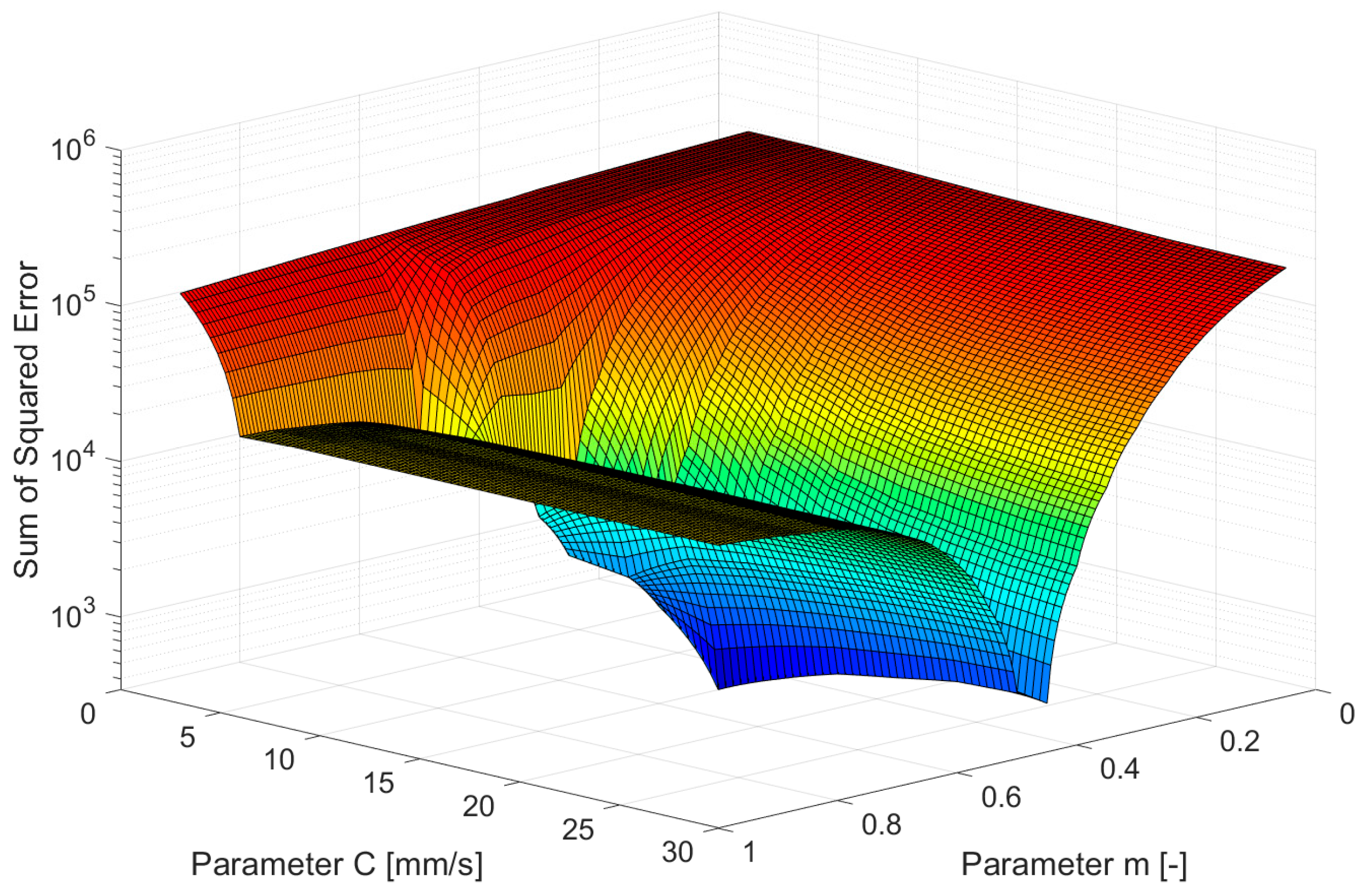
The results of previous works already showed that local minima in the cost function can occur during the inverse modeling of a two-parameter friction model, which influences the results of the inverse modeling. Therefore, before using a cost function, it makes sense to first investigate its course. For this purpose, simulation results with known friction parameters are used as a reference instead of experimental results. Subsequently, simulations are carried out with every possible combination of friction parameters, and the error value of the cost function is calculated. Plotting the error value of the cost function against each combination of friction parameters yields a cut through the cost function for the given reference data. For the creation of that cut, which is shown in Figure 3, simulation results of a simulation with m = 0.5 and C = 15 mm/s were chosen as reference data, using the simulation model with a tool speed of 30 mm/s.

However, the cut through the cost function described in Equation (2) has a large valley parallel to the axis of parameter C. Additionally, the global minimum does not differ significantly from the valley in terms of the resulting error value of the cost function. This can lead to problems in the convergence of the optimization algorithm. A valley with a low error value in this case means that different combinations of the parameters C and m lead to very similar evolutions of the sample contour so that the error value of the cost function differs only slightly from the global minimum and thus the actual solution. In this case, while m can be identified rather accurately, especially a variation of C has only a minor influence on the results due to the valley parallel to the axis of parameter C. In the conical tube-upsetting test, the specimen contour evolution is significantly influenced by the frictional stresses that occur. As mentioned, parameter m used in the friction model influences the term that considers the ratio of normal stress to yield stress, while parameter C influences the term that takes into account the prevailing relative velocity. Thus, if different values for C lead to nearly identical results, it is likely that the relative velocities occurring over the process vary only slightly. If this is the case, the friction model only has to describe one case correctly with the parameter C. This seems to be possible for several different values for C, hence, the valley in the cost function. Since parameter m can be identified accurately, the occurring normal stresses seem to vary enough along the forming process to allow only one accurate solution for m.

Figure 4 shows the average normal stress and the average relative velocity of the upper contact area over the process time of the simulation. It can be seen that the normal stresses increase from the beginning to the end of the process from 80 MPa to 180 MPa. The slight drop in the normal stress at 0.4 s process time is due to an intermediate remeshing. Remeshing is used because the degree of deformation is high, and there would otherwise be too much element distortion locally. The relative velocity, on the other hand, varies from values of approximately 5 mm/s up to approximately 12 mm/s. However, only towards the end of the forming process (≥0.4 s) an increase in the relative velocity above 7 mm/s can be recorded. Since this increase only occurs towards the end of the forming process, the change in relative velocity will have little influence on the change in the contour of the specimen since the influence also decreases with a decreasing remaining process time. Therefore, it is necessary to use a wider range of occurring relative velocities for the parameterization of the friction model so that the friction model must provide a valid solution for several cases, which in turn is only possible with a specific value for C.

4. Inverse Approach Using Multiple Upsetting Tests with Two Different Tool Velocities

In order to increase the range of relative velocities that are included in the inverse modeling, either the process windows occurring in the test must be extended, or several tests with different process conditions have to be used for the modeling. Occurring relative velocities are simple to adjust since these are significantly influenced by the tool speed and can, therefore, be changed by adjusting the punch speed. Here, on the one hand, it is possible to dynamically change the tool speed over the course of the test or to use several tests with different tool speeds as a basis for the inverse modeling. The use of one experiment with a dynamic velocity profile offers the advantage that only one experiment is included in the inverse modeling, which means that only one FE model has to be calculated per iteration. The use of two experiments with two different velocities offers the advantage of a generally larger database for inverse modeling. On the other hand, two FE models have to be calculated for each iteration of the inverse modeling, and when using experimental data as objective, the measured data of both experiments may be influenced by measurement uncertainties and fluctuations. However, since the use of two experiments and, thus, a generally larger database significantly increases the probability of obtaining a cost function with a unique minimum, this strategy was pursued in this work.

For this purpose, the inverse modeling was adapted in such a way that a test with 30 mm/s and a test with 60 mm/s tool speed are now taken into account, as shown in Figure 5. Therefore, a second simulation model with adapted tool speed must be used, which is additionally calculated for each iteration. The cost function must also be adapted accordingly to take into account the development of the specimen contour over the forming process with equal weighting for both tests:

$$\mathsf{\Phi }=\sqrt{{\displaystyle \sum }_{i=1}^t\left\{{\displaystyle \frac{1}{n}}{\displaystyle \sum }_{j=1}^n{\left(r_{ij}^{obj}-r_{ij}^{sim,30 \mathrm{mm}/\mathrm{s}}\right)}^2\right\} +{\displaystyle \sum }_{k=1}^u\left\{{\displaystyle \frac{1}{m}}{\displaystyle \sum }_{l=1}^m{\left(r_{kl}^{obj}-r_{kl}^{sim, 60 \mathrm{mm}/\mathrm{s}}\right)}^2\right\} }$$

(3)

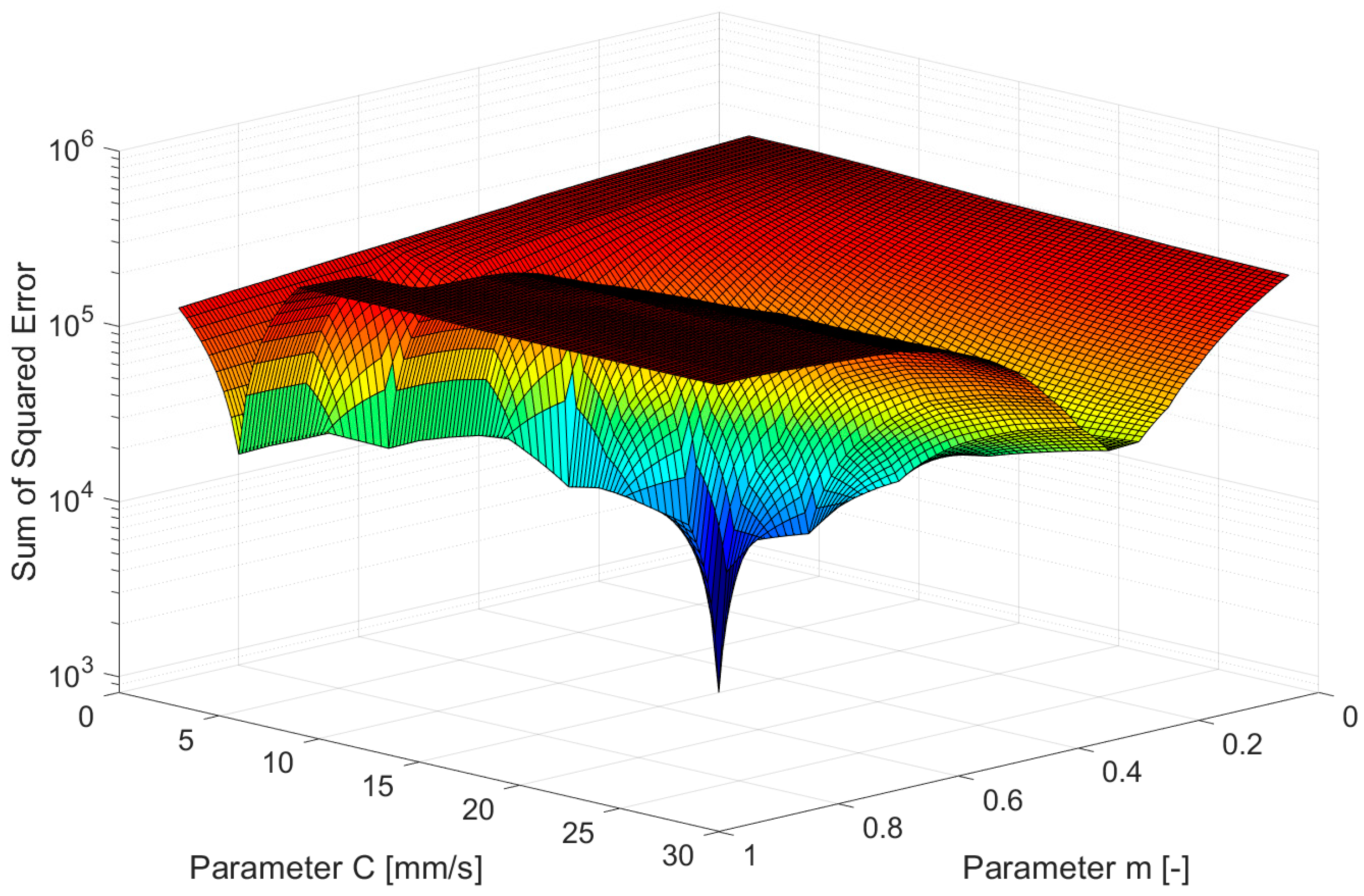
In order to investigate the course of the cost function, a cut through the cost function is created again. For this purpose, data must now be given for both models (30 mm/s and 60 mm/s) to which the cost function compares the results of the simulation models. Thus, to create the cut, simulation results of the conical tube-upsetting test were used again, with parameters set at m = 0.5 and C = 15 mm/s. Then, the value of the cost function was again calculated for all possible combinations of m and C. The corresponding error map is shown in Figure 6. There is a clear improvement in the course of the cost function compared to the cost function from Equation (2), which only considers a test with constant tool speed. There is no more deep valley, but only a global minimum at the point of the parameter combination used as objective data. Thus, the developed cost function seems to provide a promising approach for the unambiguous inverse parameterization of the chosen two-parameter friction model.

Of course, the use of simulation results as objective data serves only to investigate the course of the cost function under ideal conditions. To validate the methodology under real conditions, conical tube-upsetting tests were carried out, on the basis of which the friction model is to be parameterized by means of inverse modeling.

5. Experimental Procedure

Figure 7 shows the setup used to perform the conical tube-upsetting tests. The flat upsetting punch and the upper conical punch are each mounted on heatable elements in order to be able to heat the punches to temperatures of up to 300 °C. This allows for typical hot forging conditions to be reproduced. A centering device centered on the upper conical punch is used to center the specimen to the upper conical punch before starting the test to ensure homogeneous forming. A PLC (Programmable Logic Controller) spray system is used to apply lubricant. The spray head of the system can be swiveled under the conical punch by means of a pneumatically swiveling arm in order to coat the conical punch with a reproducible amount of lubricant at a defined system pressure and programmed pre-blow, spray, and post-blow times. A blue line laser (scanCONTROL 2750-100(506) by Micro-Epsilon Messtechnik GmbH & Co. KG, Ortenburg, Germany) with a measurement accuracy of 15 µm, which is aligned by means of a camera tripod and a reference specimen, records the outer specimen contour of the specimen with a measuring frequency of approx. 100 Hz throughout the entire test. The specimens used have an outer diameter of 30 mm and an inner diameter of 15 mm, the specimen height is 30 mm, and the cone angle is 10°. Before the start of the test, the specimen is heated in an external radiation furnace, which has been calibrated to a temperature of 1000 °C, for 10 min and then placed on the lower upsetting punch. At the same time, the swivel arm of the spray system is swiveled under the conical punch and sprayed twice with lubricant at a pressure of 2 bar and a spray time of 150 ms each. The lubricant used was Lubrodal from Fuchs Lubritech in a mixing ratio with water of 1:9. The stamps were heated to a temperature of 300 °C. Before starting the test, the specimen was centered by means of the centering device and then upset at punch velocity of 30 or 60 mm/s up to a relative height reduction of 50%. Four tests were carried out for each of the two tested velocities.

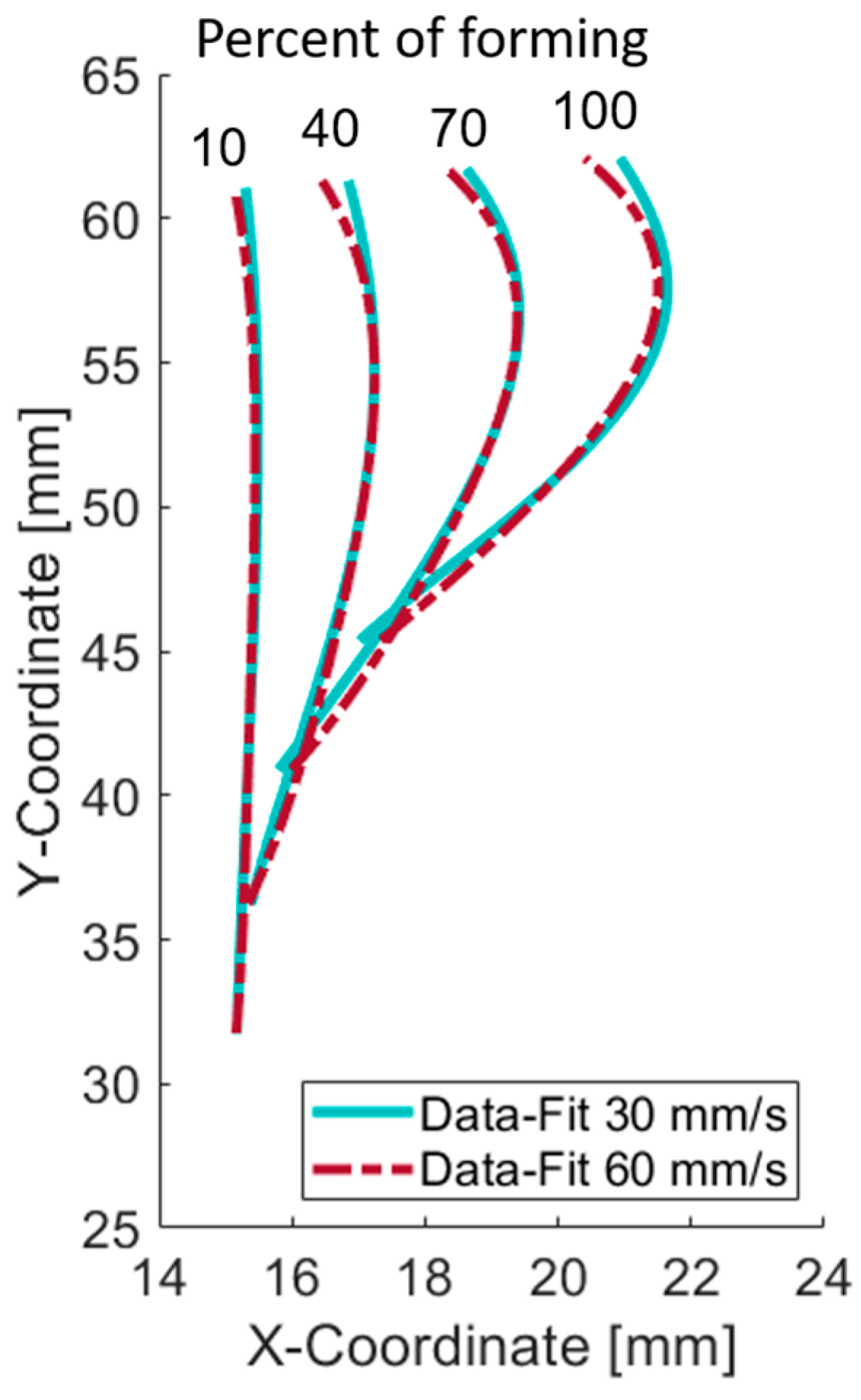
For the evaluation of the experiments, the sample contour was extracted from the laser measurement data at 10 equidistant time points from the beginning to the end of the experiment. The experiments show good reproducibility; therefore, the experimental data of the four experiments were jointly fitted to a 4th degree polynomial for each time point. Also, a clear difference regarding the evolution of the specimen contour can be seen for the experiments conducted at 30 mm/s and at 60 mm/s, showing the influence of the tool speed and, thus, of the relative velocity in the contact area, see Figure 8.

6. Inverse Modeling Using Experimental Data

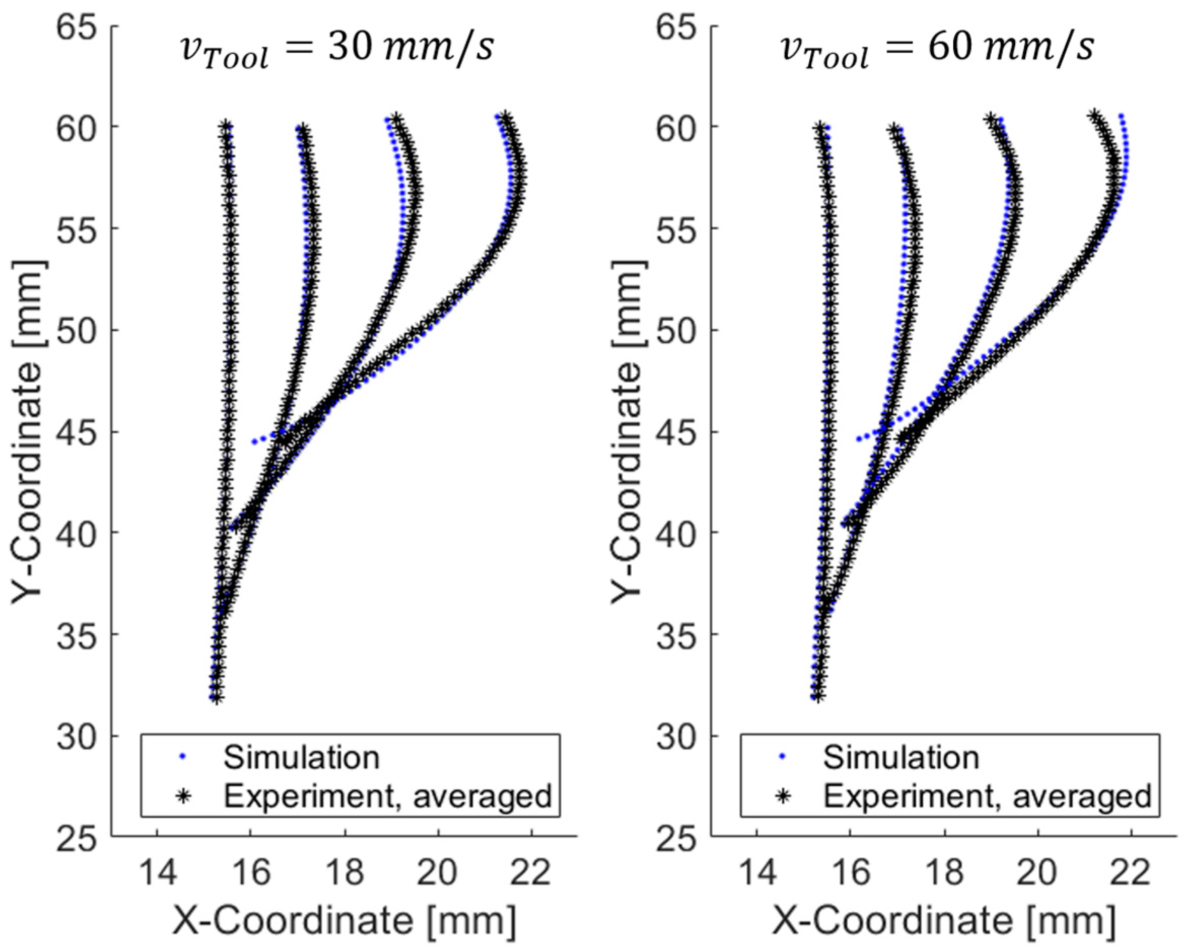
The averaged data from the tests at 30 mm/s and 60 mm/s were then used as objective data for inverse modeling, using Equation (3) as the cost function. As a starting point, the model parameters were set to m = 0.1 and C = 5.0 mm/s. The limits for the parameters were set to 0.01 < m < 1 and 1 mm/s < C < 150 mm/s. After 11 iterations, the optimization ended, resulting in final parameters of m = 0.232 and C = 85.0 mm/s. Thus, the final value for C exceeds the model author’s recommendation of the upper limit for the parameter. For the final parameters, the simulation results show a resulting maximum relative velocity of approximately 40 mm/s in the upper contact area. However, since it is just a recommendation, a reasonable upper limit for parameter C might be strongly dependent on the forming process in question. Figure 9 shows the comparison of both simulation models using the final parameters with the respective experimental data. Overall, both simulations are in good agreement with the experimental data. Minor deviations are to be expected for a comparison between simulation and experimental data. The biggest deviations can be seen at 100%, forming a tool velocity of 60 mm/s.

Increasing deviations towards the end of the forming process can be explained by frictional conditions having an increasing influence on the resulting specimen contour the further the forming process advances. For the conical tube-upsetting test, especially the upper part of the specimen is sensitive to friction. The lower the friction, the greater the resulting change in radius (X-coordinate). Especially for the later forming stages, it can be observed that the simulation underestimates the experimental displacement in the X-direction for 30 mm/s while it overestimates the displacement in the X-direction for 60 mm/s. One possible explanation is that the used friction model is not completely capable of describing the velocity dependency for the given process and process conditions. Secondly, deviations could also be caused by experimental uncertainties. Finally, the finally determined parameters of the friction model might not be the optimal solution, i.e., the global minimum of the cost function.

Since the focus of this work lies in method development, validating the determined parameters in terms of being the cost functions minimum is necessary. Therefore, another cut through the cost function was calculated, this time using the experimental data as an objective. The calculated cut is shown in Figure 10. The cut shows a minimum of around m ≈ 0.23 and C ≈ 90 mm/s. This confirms that the proposed method is capable of finding the minimum for experimental data, not exactly, but at least with reasonable accuracy. It is also noteworthy that the cut again shows a valley parallel to the axis of parameter C. The valley explains why the optimization process had trouble finding the global minimum of the cost function. It also supports the thesis that the used model cannot perfectly describe the velocity dependency for both experiments with one value of C, either due to the nature of the model or due to experimental inaccuracies. The model has a velocity dependency and was originally developed and validated for processes with a higher velocity, so it cannot be ruled out that the friction model cannot optimally map the existing conditions. However, small inaccuracies can also occur due to the experimental procedure, such as the centering or transferring time of the specimen. Nevertheless, this suggests that the proposed method is well capable of determining the parameters of a two-parameter friction model.

7. Conclusions

The goal of this work was to develop a methodology for the calibration of two-parameter friction models using inverse modeling of conical tube-upsetting tests. The conical tube-upsetting test is a laboratory test for the investigation of friction under process conditions of bulk metal forming.

An inverse method was presented, where the developing outer contour of the conical tube-upsetting test is compared to an FE model. The difference between simulation and experimental objective data is calculated, which is, in turn, minimized by an optimization algorithm. The method was investigated under ideal conditions, using simulation results as objective data for the cost function. As for friction modeling, a two-parameter model was chosen. The results for this approach suggest that the relative velocities occurring during forming did not vary enough throughout the process to result in a unique solution for the model parameters. Therefore, the used cost function was adjusted, considering two tests with different tool velocities and, thus, different relative velocities. Using simulation results as objective data, the method suggested an improvement towards the first approach, resulting in a unique solution for the identification of the model parameters.

In the next step, experimental data were generated, conducting conical tube-upsetting tests at two different tool velocities to serve as the objective for the optimization process. For this, the algorithm was also able to determine optimal parameters. An investigation of the shape of the cost function confirms that the developed method is capable of finding the global minimum of the cost function within reasonable accuracy. Thus, the presented method gives a promising approach to the calibration of two-parameter friction models.

In general, the basic principles of the presented approach could be transferred to other friction models or laboratory tests in the future. For future work, the application of the developed method for the determination of model parameters for friction-sensitive forming processes is planned.

References

1. Bay, N. Friction Stress and Normal Stress in Bulk Metal-Forming Processes. J. Mech. Work. Technol. 1987, 14, 203–223. [Google Scholar] [CrossRef]
2. Nielsen, C.V.; Bay, N. Overview of friction modelling in metal forming processes. Procedia Eng. 2017, 207, 2257–2262. [Google Scholar] [CrossRef]
3. Orowan, E. The Calculation of Roll Pressure in Hot and Cold Flat Rolling. Proc. Inst. Mech. Eng. 1943, 150, 140–167. [Google Scholar] [CrossRef]
4. Bay, N.; Wanheim, T. Real Area of Contact and Friction Stress at High Pressure Sliding Contact. Wear 1976, 38, 201–209. [Google Scholar] [CrossRef]
5. Bay, N.; Wanheim, T. Contact Phenomena under Bulk Plastic Deformation Conditions. In Proceedings of the Third International Conference on Technology of Plasticity: Advanced Technology of Plasticity, Kyoto, Japan, 1–6 July 1990; Japan Society for Technology of Plasticity: Tokyo, Japan, 1990; pp. 1677–1691. [Google Scholar]
6. Chen, C.C.; Kobayashi, S. Rigid Plastic Finite Element Analysis of Ring Compression. Appl. Numer. Methods Form. Process. 1978, 28, 163–174. [Google Scholar]
7. Behrens, B.-A.; Alasti, M.; Bouguecha, A.; Hadifi, T.; Mielke, J.; Schäfer, F. Numerical and experimental investigations on the extension of friction and heat transfer models for an improved simulation of hot forging processes. Int. J. Mater. Form. 2009, 2, 121–124. [Google Scholar] [CrossRef]
8. Behren Bouguecha, A.; Mielke, J.; Hirt, G.; Bambach, M.; Al Baouni, M.S.H.; Demant, A. Verbesserte numerische Prozesssimulation mittels eines innovativen Reibgesetzes für die Warmmassivumformung: Improved numerical process simulation by means of an innovative friction law for hot forging. Schmiede-J. März 2010, 20–24. [Google Scholar]
9. Behrens, B.-A.; Bouguecha, A.; Hadifi, T.; Mielke, J. Advanced friction modeling for bulk metal forming processes. Prod. Eng. 2011, 5, 621–627. [Google Scholar] [CrossRef]
10. Tan, X. Comparisons of friction models in bulk metal forming. Tribol. Int. 2002, 35, 385–393. [Google Scholar] [CrossRef]
11. Joun, M.; Moon, H.; Choi, I.; Lee, M.; Jun, B. Effects of Friction Laws on Metal Forming Processes. Tribol. Int. 2009, 42, 311–319. [Google Scholar] [CrossRef]
12. Henke, T.; Hirt, G.; Bambach, M. Randwertermittlung für die robuste Auslegung von Schmiedeprozessen. Wt Werkstattstech. Online 2013, 103, 783–788. [Google Scholar] [CrossRef]
13. Lenard, J.G. Tribology in Metal Rolling Keynote Presentation Forming Group F. CIRP Ann. 2000, 49, 567–590. [Google Scholar] [CrossRef]
14. Dellah, A.; Wild, P.M.; Moore, T.N.; Shalaby, M.; Jeswiet, J. An Embedded Friction Sensor Based on a Strain-Gauged Diaphragm. J. Manuf. Sci. Eng. 2002, 124, 523–527. [Google Scholar] [CrossRef]
15. Masters, I.G.; Williams, D.K.; Roy, R. Friction behaviour in strip draw test of pre-stretched high strength automotive aluminium alloys. Int. J. Mach. Tools Manuf. 2013, 73, 17–24. [Google Scholar] [CrossRef]
16. Mandic, V.; Stefanovic, M. Friction Studies Utilizing the Ring—Compression Test—Part I. Tribol. Ind. 2003, 25, 33–40. [Google Scholar]
17. Mandic, V.; Stefanovic, M. Friction Studies Utilizing the Ring—Compression Test—Part II. Tribol. Ind. 2003, 25, 76–82. [Google Scholar]
18. Plančak, M.; Car, Z.; Kršulja, M.; Vilotić, D.; Kačmarčik, I.; Movrin, D. Possibilities To Measure Contact Friction In Bulk Metal Forming. Teh. Vjesn. Tech. Gaz. 2012, 19, 727–734. [Google Scholar]
19. Male, A.T.; DePierre, V. The Validity of Mathematical Solutions for Determining Friction From the Ring Compression Test. J. Lubr. Technol. 1970, 92, 389–395. [Google Scholar] [CrossRef]
20. Kopp, R.; Al Baouni, M.S.H.; Volles, R. Conical Tube Upsetting Test—A New Method for Accurate Determination of The Friction Coefficient. In Proceedings of the 8th International Conference on Technology of Plasticity, Verona, Italy, 9–13 October 2005. [Google Scholar]
21. Kopp, R.; Philipp, F.-D. Physical parameters and boundary conditions for the numerical simulation of hot forming processes. Steel Res. 1992, 63, 392–398. [Google Scholar] [CrossRef]
22. Teller, M.; Klubakov, A.; Franzke, M.; Lohmar, J.; Hirt, G. Extended Conical Tube-Upsetting Test to Investigate the Evolution of Friction Conditions. Key Eng. Mater. 2016, 716, 157–164. [Google Scholar] [CrossRef]
23. Szeliga, D.; Gawad, J.; Pietrzyk, M. Inverse analysis for identification of rheological and friction models in metal forming. Comput. Methods Appl. Mech. Eng. 2006, 195, 6778–6798. [Google Scholar] [CrossRef]
24. Szeliga, D.; Gawąd, J.; Pietrzyk, M. Parameters identification of material models based on the inverse analysis. Int. J. Appl. Math. Comput. Sci. 2004, 14, 549–556. [Google Scholar]
25. Cho, H.; Ngalle, G.; Altan, T. Simultaneous Determination of Flow Stress and Interface Friction by Finite Element Based Inverse Analysis Technique. CIRP Ann. 2003, 52, 221–224. [Google Scholar] [CrossRef]
26. Henze, M.; Teller, M.; Hirt, G. Parametrization of Bi-Parametric Friction Models Through Inverse Modelling of Conical Tube-Upsetting Tests. AIP Conf. Proc. 2019, 2113, 120002. [Google Scholar]
27. Spittel, M.; Spittel, T. Steel symbol/number: 18CrNiMo7–6/1.6587, In Metal Forming Data of Ferrous Alloys—Deformation Behaviour; Martienssen, W., Warlimont, H., Eds.; Springer: Berlin/Heidelberg, Germany, 2009; pp. 984–989. [Google Scholar] [CrossRef]
28. Byrd, R.H.; Schnabel, R.B.; Shultz, G.A. Approximate solution of the trust region problem by minimization over two-dimensional subspaces. Math. Program. 1988, 40, 247–263. [Google Scholar] [CrossRef]
29. MathWorks. Optimization Toolbox: User’s Guide. Available online: https://de.mathworks.com/help/optim/ug/least-squares-model-fitting-algorithms.html (accessed on 14 November 2024).
30. Moré, J.J.; Sorensen, D.C. Computing a Trust Region Step. SIAM J. Sci. Stat. Comput. 1983, 4, 553–572. [Google Scholar] [CrossRef]
Figure 1. Specimen before and after compression and schematic of the experimental setup for the conical tube-upsetting test.
Metals 14 01355 g001
Figure 2. Flow chart for the inverse modeling of conical tube-upsetting test.
Metals 14 01355 g002
Figure 3. Cut through the cost function using the numerical data at m = 0.5 and C = 15 mm/s as objective and calculated Equation (2) with a tool speed of 30 mm/s.
Metals 14 01355 g003
Figure 4. Average normal stress and average relative velocity in upper contact surface for a simulation of a conical tube-upsetting test with a tool speed of 30 mm/s (m = 0.5; C = 30 mm/s).
Metals 14 01355 g004
Figure 5. Flow chart for the inverse modeling of conical tube-upsetting test using two tests with different velocities.
Metals 14 01355 g005
Figure 6. Cut through the cost function using the numerical data at m = 0.5 and C = 15 mm/s as objective and calculated Equation (3) with a tool speed of 30 mm/s and 60 mm/s.
Metals 14 01355 g006
Figure 7. Experimental setup used for the conical tube-upsetting tests while lubricating the upper punch (left) and prior to deformation of a specimen (right).
Metals 14 01355 g007
Figure 8. Comparison of outer specimen contour at 10%, 40%, 70%, and 100% of forming for fitted experimental data with different tool velocities.
Metals 14 01355 g008
Figure 9. Comparison of outer specimen contour at 10%, 40%, 70%, and 100% of forming for simulation and experiment at 30 mm/s tool velocity (left) and 60 mm/s tool velocity (right) with m = 0.232 and C = 85.0 mm/s.
Metals 14 01355 g009
Figure 10. Cut through the cost function using Equation (3) and the experimental data as objective with a tool speed of 30 mm/s and 60 mm/s.
Metals 14 01355 g010