Article

Study on the Process Window in Wire Arc Additive Manufacturing of a High Relative Density Aluminum Alloy

1
School of Mechanical Engineering, Xi’an Jiaotong University, Xi’an 710049, China
2
National Innovation Institute of Additive Manufacturing, Xi’an 710100, China
*
Author to whom correspondence should be addressed.
Metals 2024, 14(3), 330; https://doi.org/10.3390/met14030330
Submission received: 8 February 2024 / Revised: 8 March 2024 / Accepted: 10 March 2024 / Published: 13 March 2024

Abstract

:
In recent years, there has been a heightened focus on multiplex porosity due to its significant adverse impact on the mechanical properties of aluminum alloy components produced through wire arc additive manufacturing (WAAM). This study investigates the impacts of the process parameters and dimension parameters on the relative densities of WAAM 2219 aluminum alloy components by conducting experiments and investigates the changes in high relative density process windows with different dimension parameters. The findings reveal a hierarchy in the influence of various parameters on the relative density of the 2219 aluminum alloy: travel speed (TS), wire feed speed (WFS), the number of printed layers (L), interlayer cooling time (ICT), and theoretical length of weld (TLW). A series of data for analysis was produced through a designed experiment procedure, and on the basis of this, by integrating the data augmentation method with the eXtreme Gradient Boosting (XGBoost) algorithm, the relationship among the process parameters, dimension parameters, and relative density was modeled. Furthermore, through leveraging the established model, we analyzed the changes in the optimized process window corresponding to a high relative density with the L. The optimal windows of WFS and TS change when the L reaches a certain value. In contrast, the optimal window of ICT remains consistent despite an increase in the L. Finally, the relative density and mechanical properties of the formed 20-layer specimens within the model-derived window were verified. The relative density of the specimens within the window reached 98.77%, the ultimate tensile strength (UTS) reached 279.96 MPa, and the yield strength (YS) reached 132.77 MPa. This work offers valuable insights for exploring the process window and selecting process parameters through a more economical and faster approach in WAAM aluminum components.

1. Introduction

Wire arc additive manufacturing (WAAM) uses arc welding as a heat source and filler wire as a feedstock to manufacture a component using the layer-by-layer deposition method [1], which can realize the manufacturing of large-sized parts [2] and is widely used in the marine, aerospace, and automotive fields [3,4,5]. However, various defects, such as a high porosity, residual stress, and cracking, constrain the application of this promising AM method [5]. The 2219 aluminum alloy is an age-hardening Al–Cu alloy, which has good mechanical properties in the temperature range of −250–300 °C [6,7]. Spherical θ″-Al2Cu particles and flaky-like θ′-Al2Cu precipitates are components of the main strengthening phases, and the α-Al + θ-Al2Cu eutectic phase has an important effect on the properties of the alloy [8,9]. Generally, the α-Al phase presents columnar and equiaxed dendrites, the network-like α-Al + θ-Al2Cu eutectic phases are distributed along grain boundaries and interdendrite regions, and θ′ and θ″ are distributed in the Cu-rich region near the eutectic α-Al + θ-Al2Cu [9]. For aluminum alloys, multiplex porosities threaten the quality significantly. They exhibit different quantitative and morphological characteristics at different positions of the components, while their quantitative and morphological characteristics change after heat treatment [10]. In addition, deposited alloys also show different defect levels under different process parameters [11].
Ryan et al. [12] investigated the effects of wire batches, cold metal transfer (CMT) transfer modes, wire feed speed (WFS), and travel speed (TS) on the porosity of the WAAM 2319 aluminum alloy. The results showed that the surface finish of the wire affects the wire surface’s hydrogen content and arc stability, which affects the porosity. Hauser et al. [13] showed that a higher shielding gas flow rate inhibits a decrease in porosity in the molten pool, resulting in a higher porosity inside the WAAM aluminum alloy component. Derekar et al. [14] investigated the effects of different interlayer temperatures on the porosity, and the results showed that the specimens at higher interlayer temperatures had a lower porosity. At present, the acquisition of optimized process parameters usually relies on experiments [15,16,17] or numerical calculations [18,19], which are costly. In addition, most studies do not consider variations of optimal process parameters with different size parameters. At the same time, due to the complex formation mechanism, it is difficult to simulate the pore defects in WAAM components by building physical models.
Machine learning (ML) methods do not need to consider the actual physical process and have a good learning ability for nonlinear processes. The application of ML in the field of additive manufacturing has gradually increased in recent years. Xiao et al. [20] used neural networks to establish a bidirectional prediction model between the WAAM process parameters and weld morphology, which can realize back calculations of the optimized process parameters from the desired process quality level. Dharmawan et al. [21] used reinforcement learning to correct the prediction of the layer heights for each layer in the WAAM process and obtained a WAAM bronze block with a flatter upper surface. Ling et al. [22] combined physical modeling and ANN to achieve the predictions of the microstructure and hardness of WAAM low-carbon steel components. In the LPBF process, Tapia et al. [23] used Gaussian regression to realize the prediction of the porosity under any combination of laser power and scanning speed in the LPBF process. Liu et al. [24] used Gaussian regression to predict the relative density of the AlSi10Mg sample manufactured by LPBF and obtained a new process window. The new process window can obtain samples with a high tensile strength and elongation without heat treatment. Compared with the application of machine learning in laser additive manufacturing, its application in WAAM is mostly in the optimization of the specimen’s morphology, and there are few studies on the optimization of the relative density.
This paper studies the acquisition of the process window for a WAAM aluminum alloy with a high relative density as well as variations of process windows with different dimension parameters (number of printing layers (L)). In this study, we research the impacts of different process parameters and dimension parameters on the relative density of WAAM 2219 aluminum alloy. Combined with a generative adversarial network with a gradient penalty term (WGAN-GP), the model of the process parameters, dimension parameters, and relative density was established using eXtreme Gradient Boosting (XGBoost). Then, variations of the optimized window of process parameters with different numbers of printed layers (Ls) were analyzed based on the model. Finally, the relative density and mechanical properties of the samples corresponding to the window obtained using the model were verified.

2. Theory and Methods

2.1. Experimental Methods

In this section, orthogonal experiments were designed to study the effects of the process parameters and size parameters on the relative densities of the deposited alloys. In order to analyze the spatial distribution of the pore defects and microstructures in the sample, a CT test was performed on the top–middle area of the sample, the 5 mm × 5 mm × 5 mm squares were extracted from each sample, and their microstructure was observed under an optical microscope. In addition, the verification experiment settings for the relative density and mechanical properties of the sample in the optimal process window obtained later are also explained in this section. The material used for the experiment was GR-2319 aluminum wire, and the substrate used was a 100 mm × 100 mm × 20 mm 2219-T6 aluminum alloy plate. The composition of the wire is listed in Table 1. The manufacturing process was carried out using the CMT additive manufacturing system, which is mainly composed of a Fronius-CMT Advanced 4000, a wire feeder, and a KUKA KR16 robot. The CMT-P mode was used in the wire and arc additive manufacturing (WAAM) process, the shielding gas was 99.99% Ar, and the flow rate of the shielding gas was 25 L·min−1.
The relative density of the WAAM walls stable section was measured using the Archimedes drainage method according to the GB/T 3850-2015 standard [25], and the theoretical density of the material, ρtheory = 2.84 g·cm−3. Before the relative density test, the unstable areas at the arc starting and arc quenching points were removed. The surface of the samples was polished with 80# sandpaper, and then the samples were cleaned in an alcohol solution for 5 min using an ultrasonic cleaning machine. The relative density was measured using a DH-220MN electronic balance. In the as-deposited thin-walled walls, the pore diameter in the top region is the largest [8]. Therefore, after testing the relative density, a column with a length of 15 mm and a height equal to the width of the deposited sample was taken from the top of each sample for CT testing, to characterize the spatial distribution characteristics of the pores. The CT model used was the Phoenix v|tome|x m, in which the maximum detection size is Φ400 mm × H420 mm, and the resolution during detection was set to 17 μm. The microstructures of the samples and the two-dimensional morphologies of the pores were observed with a Zeiss Axio Vert.A1 inverted optical microscope. The metallographic sample was polished with 80#, 240#, 400#, 800#, 1200#, and 2000# sandpaper, and after polishing, the surface was etched with Keller’s reagent. The sampling position of each test in the experiment is shown in Figure 1. For the mechanical properties of the experiment in accordance with Figure 2, to prepare the tensile specimens, an Instron 5982 mechanical testing machine was used at room temperature to carry out the mechanical property testing, at tensile rate of 0.5 mm·min−1. The wire feed speed (WFS), travel speed (TS), interlayer cooling time (ICT), the number of printed layers (L), and theoretical length of weld (TLW) were selected as variables to design orthogonal experiments, where the TLW is the distance from the arc starting point to the arc extinguishing point. The values of each parameter are listed in Table 2.

2.2. eXtreme Gradient Boosting Algorithm

The relationship model between the printing parameters and the relative density was established using the eXtreme Gradient Boosting (XGBoost) method, which is an integrated algorithm based on the idea of boosting and consists of multiple regression trees. Each tree is trained in turn during the training process, and the result of the last tree is the final result of the XGBoost model, which is expressed as follows:
y ^ i ( K ) = k = 1 K f k ( x i ) = k = 1 K 1 f k ( x i ) + f K ( x i )
where  y ^ i ( K )  is the predicted value of the model for sample i, and K is the total number of trees. The objective function of XGBoost can be described by:
( w 1 * , w 2 * , , w m * ) = arg min i = 1 N L ( y i , y ^ i ( k ) ) + k = 1 K Ω ( f k )
where w1*, w2*, and wm* denote the output results of the nodes, and K is the current total number of trees. The expression of the regular term  k = 1 K Ω ( f k )  is described as follows:
k = 1 K Ω ( f k ) = k = 1 K 1 Ω ( f k ) + Ω ( f K )
Ω ( f K ) = γ T + 1 2 λ j = 1 T w j 2
where T is the number of leaf nodes in the current tree, and wj denotes the value of the jth leaf node. λ and γ are hyperparameters.
Expanding the first term in Equation (2) using a 2nd-order Taylor expansion results in a final objective function of XGBoost as follows:
O b j k = γ T + j = 1 T [ G j w j + 1 2 ( H j + λ ) w j 2 ]
In the formula,  G j = i I j L ( y i , y ^ i ( k 1 ) )  and  H j = i I j L ( y i , y ( k 1 ) ) . The optimal tree structure is determined by calculating the gain after node splitting under different splitting methods. The greater the gain, the better the current way of dividing nodes. The gain of XGBoost is described as follows:
g a i n = O b j * f O b j * b
where Obj*f is the objective function value before the node splits, and Obj*b is the objective function value after the node splits. Specific theoretical references to XGBoost are found in [26,27].
The implementation of the model relied on Python 3.10 and the XGboost library. The mean squared error loss function was chosen as the loss function for the XGBoost model during the model building process, and the genetic algorithm integrated with the Geatpy library was utilized for hyper-parameter optimization in the hyper-parameter optimization process. The data obtained from the experiments were divided into a training set and a test set according to a ratio of 8:2. The 10-fold cross-validation was used for training, and the mean absolute error (MAE) and coefficient of determination (R2) were used to evaluate the model, in which
M A E = 1 m i = 1 m | y i y ^ i |
R 2 = 1 i = 1 m ( y i y ^ i ) 2 i = 1 m ( y i y ¯ ) 2

2.3. Wasserstein Generative Adversarial Networks with Gradient Penalty Terms

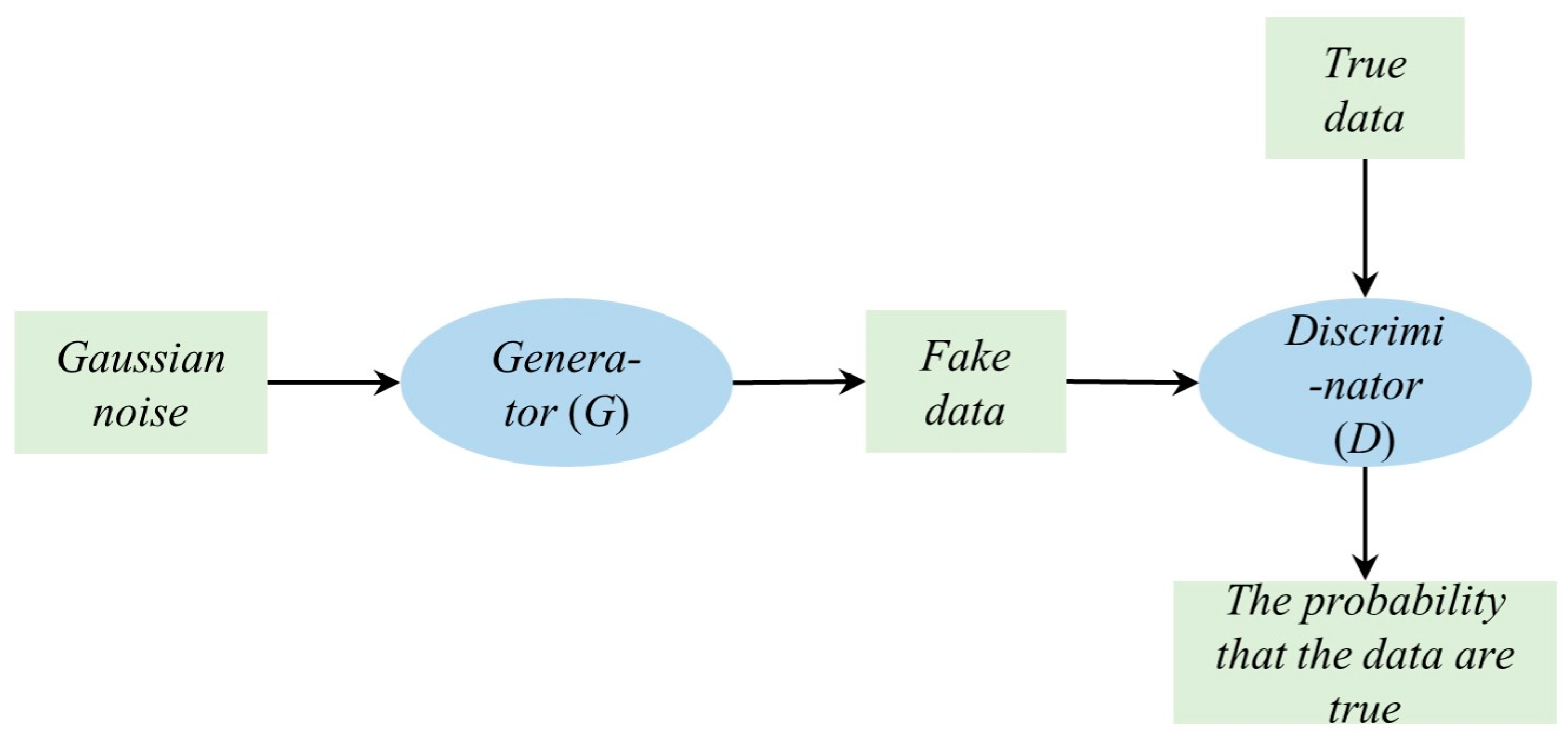
In order to improve the generalization performance of the model, data augmentation was performed on the training set data using the Wasserstein generative adversarial network with a gradient penalty term (WGAN-GP), which was implemented in the Keras framework. Wasserstein distance and gradient penalty terms are introduced into WGAN-GP to avoid gradient disappearance and model training difficulties during generative adversarial network (GAN) training [28]. Figure 3 shows the structure of the WGAN-GP. In the training process, the noise is input to the generator, which learns the distribution of the real data and outputs data similar to the real data. The real data and the generated data are used as inputs to the discriminator, which outputs the probability that the samples are real data. The target of the generator is to make the discriminator unable to clearly distinguish whether the sample is real data or generated data, whereas the target of the discriminator is to be able to correctly distinguish real data and generated data as much as possible. The objective loss function of the WGAN-GP is described as follows [28,29]:
L = E x ˜ ~ g [ D ( x ˜ ) ] E x ~ r [ D ( x ) ] + λ E x ^ ~ x ^ [ ( | | x ^ D ( x ^ ) | | 2 1 ) 2 ]
where  x ˜  is the generated data, x is the real data,  g  and  r  denote the geometric edges of all possible joint distributions of the generated data and the real data, and  x ^  is the straight line uniform sampling distribution between  g  and  r  pairs of sampling points. When the discriminator cannot distinguish between the real data and the generated data, the training is over, and the objective loss function oscillates around 0 at this time.
The real data were vectors (WFS, TS, L, ICT, TLW, and relative density)T, the input to the generator was a 6-dimensional gaussian noise, and the output was the “generated data”, whose “shape” was the same as the real data. The input to the discriminator was the real data and the generated data, and the output was the probability of representing the generated input data as real data. The generator and discriminator of the WGAN-GP were constructed using a one-dimensional convolutional network and a fully connected layer. The specific composition of the WGAN-GP is presented in Table 3. The hybrid data obtained by splicing the generated data with the real data were used to train the print parameter–relative density relationship model. To ensure the quality of the data used to train the model, the hybrid data were sorted according to their similarity, and the data with a higher similarity were selected for training the model. The similarity was calculated using the following equations [28]:
( X i t r u e , X j f a k e ) = k = 1 n ( x i , k t r u e x j , k f a k e ) 2 + ( y i t r u e y j f a k e ) 2 = ( ( x i , 1 t r u e x j , 1 f a k e ) 2 + + ( x i , n t r u e x j , n f a k e ) 2 + ( y i t r u e y j f a k e ) 2
S i m j = max { 1 1 + d i s ( X 1 t r u e , X j f a k e ) , 1 1 + d i s ( X 2 t r u e , X j f a k e ) , , 1 1 + d i s ( X n t r u e , X j f a k e ) }
where dis(Xitrue, Xjfake) is the distance between the real data and the generated data, Simj is the similarity of sample j among the mixed data, and n indicates the number of real samples. When the similarity of a sample in the mixed data is 1, it indicates that the sample is real data.

3. Results and Discussion

3.1. Effects of Print Parameters on Relative Density

The values of the relative density measured of the experiment are summarized in Table 4. In order to analyze the influence of each parameter on the relative density, a range analysis was carried out, and the results are displayed in Table 5. In Table 5, K1jK4j is the sum of the relative density measured for each parameter at different levels. k1jk4j is the mean value of the relative density measured for each parameter at different levels. j represents different parameters. As a mixed orthogonal table was used in the experiment, the final range R′ was converted using the following equation:
R = d R r
where d is the conversion coefficient, which is 0.45 for the WFS, TS, L, and ICT, and 0.71 for the TLW. R is the original range. r is the number of repetitions of the same level experiment, which is 8 for the WFS, TS, L, and ICT, and 2 for the TLW. As can be seen from the table, the TS has the greatest influence on the relative densities of the specimens, corresponding to a range of 0.91, and the TLW has the smallest influence on the relative density, with a range of only 0.03. At the same time, the L has a greater influence on the relative densities of the specimens, with a range of 0.64. The order of the parameter ranges, from the largest to the smallest, is as follows: TS > WFS > L > ICT >TLW.
Figure 4 shows the microstructures of the samples, which were observed using an optical microscope. The samples were reordered according to the size of the heat input (HI). The heat input is calculated as follows [30]:
H I = η U i I i T S
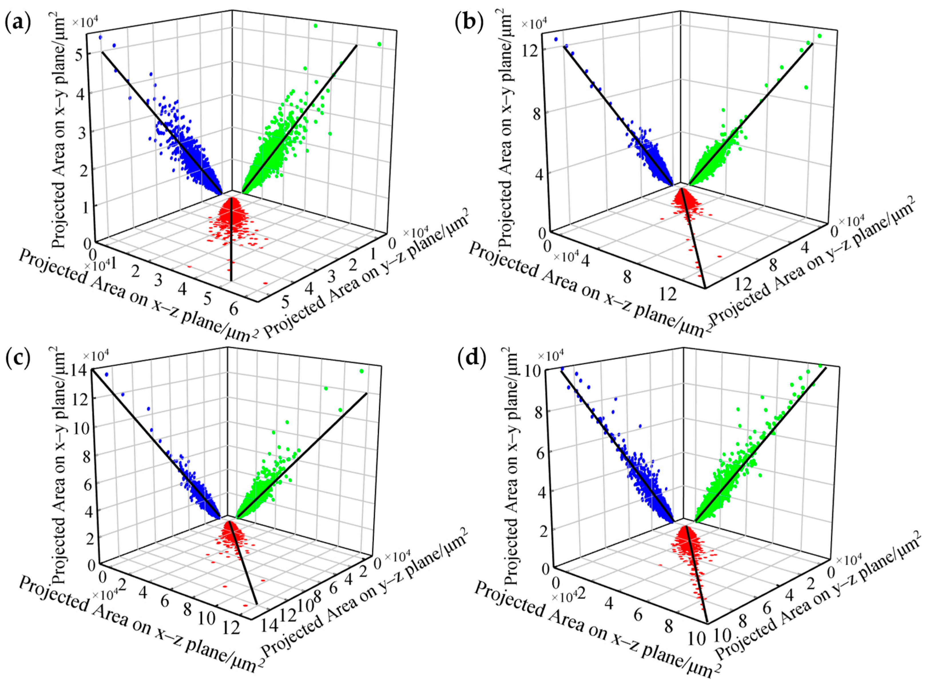
where η is thermal efficiency, η = 0.8 [29]. Ui is the voltage, and Ii is the current. TS is the travel speed. As can be seen from Figure 4, in the two-dimensional plane, the pores in the sample are usually circular in shape. Gu et al. [10] pointed out that spherical or irregularly shaped micropore defects are primarily formed by the entrapped hydrogen. This indicates that the pore defects in the sample are mainly hydrogen pores. Sanaei et al. [31] determined the expansion plane of the defect by comparing the projected area of the defect on the orthogonal plane of space. Figure 5 shows the projected area distribution of the pore defects on the spatial reference plane. The points falling on the black line in Figure 5 indicate that the projected areas of the pore defects on the two adjacent reference planes are equal, and such defects do not show obvious expansion planes. By comparing the projected areas of all samples defects, it is found that most samples have the same projected areas on the three datum planes, and this distribution is shown in Figure 5a,b. However, the defects in samples 1 and 17 have a larger projected area on the x–y plane than on the x–z and y–z planes. This indicates that the defects in samples 1 and 17 spread along the x–y plane. Wu et al. [32] pointed out that the maximum dimension direction of unfused defects is usually approximately perpendicular to the direction of accumulation. It is further indicated that unfused defects occured in samples 1 and 17. According to the experimental parameters, the L of sample 1 is the minimum value (5 layers), while the interlayer cooling time of sample 17 is the maximum value (180 s). In addition, the heat input of the two samples is less than 400 J·mm−1, which makes the samples 1 and 17 have a large temperature gradient at the same time as having a low energy input, resulting in the defects in the samples, mainly unfused defects.
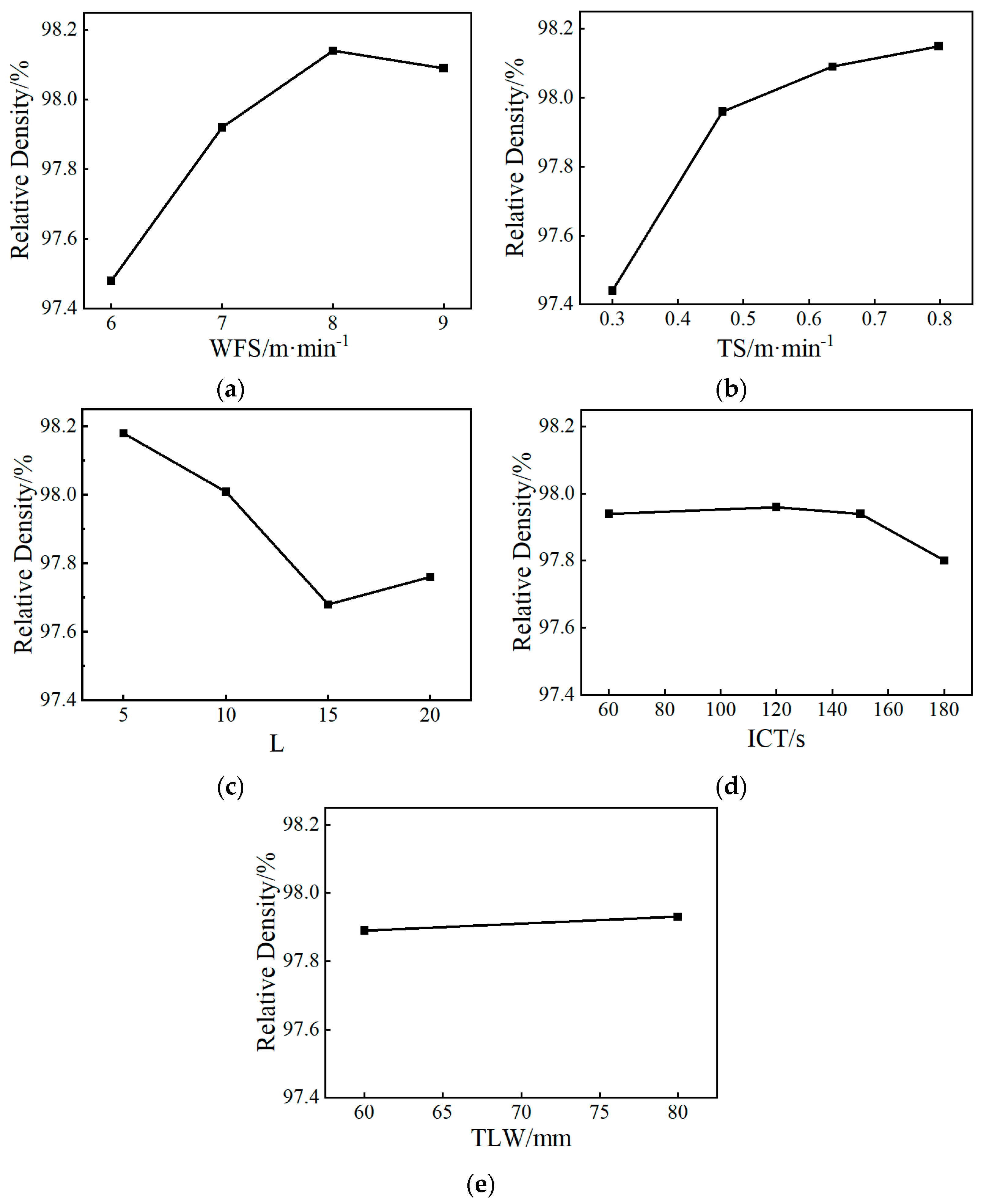
Figure 6 shows the variations in relative densities with the WFS, TS, L, ICT, and TLW. As the WFS increases, the relative density increases and then decreases, achieving a maximum value at 8 m·min−1. The smaller the WFS, the smaller the voltage and current. As can be seen from Equation (13), the lower the voltage and voltage, the smaller the HI. The analyses in Figure 4 and Figure 5 show that when the heat input is not very large and the temperature gradient is large, unfused defects may occur in the sample. Therefore, a smaller WFS reduces the line energy in the manufacturing process, increasing the likelihood of unfused defects. However, too large of a WFS will increase the temperature of the molten pool. The solubility of the hydrogen in Al–Cu alloys increases with an increasing temperature [33]. The high melt pool temperature causes the melt pool precipitate too much hydrogen and form hydrogen pores to reduce the relative density. When the TS increases, the heat input decreases, and the melt pool becomes shallower. This is more conducive to the overflow of gas pores, and the pores precipitated during metal solidification decrease, resulting in an increase in the relative density. With the increase in the L, the solidification rate of the molten pool slows down, and the dissolved hydrogen in the melt pool increases, but the solidification time is not enough to make the pores escape. The formation of hydrogen pores causes the relative density to decrease, and the lowest value is achieved in 15 layers. After 15 layers, the heat accumulation effect obviously prolongs the solidification time, allowing some pores to escape and increasing the relative density. When the ICT is between 60–150 s, the change in the ICT has little effect on the relative density. When the ICT between layers increases from 150 s to 180 s, the temperature gradient between the current layer and the previous layer increases, and the cooling rate of the melt pool becomes larger, so that some pores are unable to escape and the relative density decreases. In addition, under the combination of a high cooling rate and a low heat input, unfused defects may also appear in the sample. When the TLW increases, the arc time becomes longer. The temperature of the specimen is higher, which slows down the solidification of the melt pool to a certain extent. This is conducive to the loss of some pores and makes the relative density of the specimen increase slightly.

3.2. Modeling of Process Parameter–Relative Density Relationships

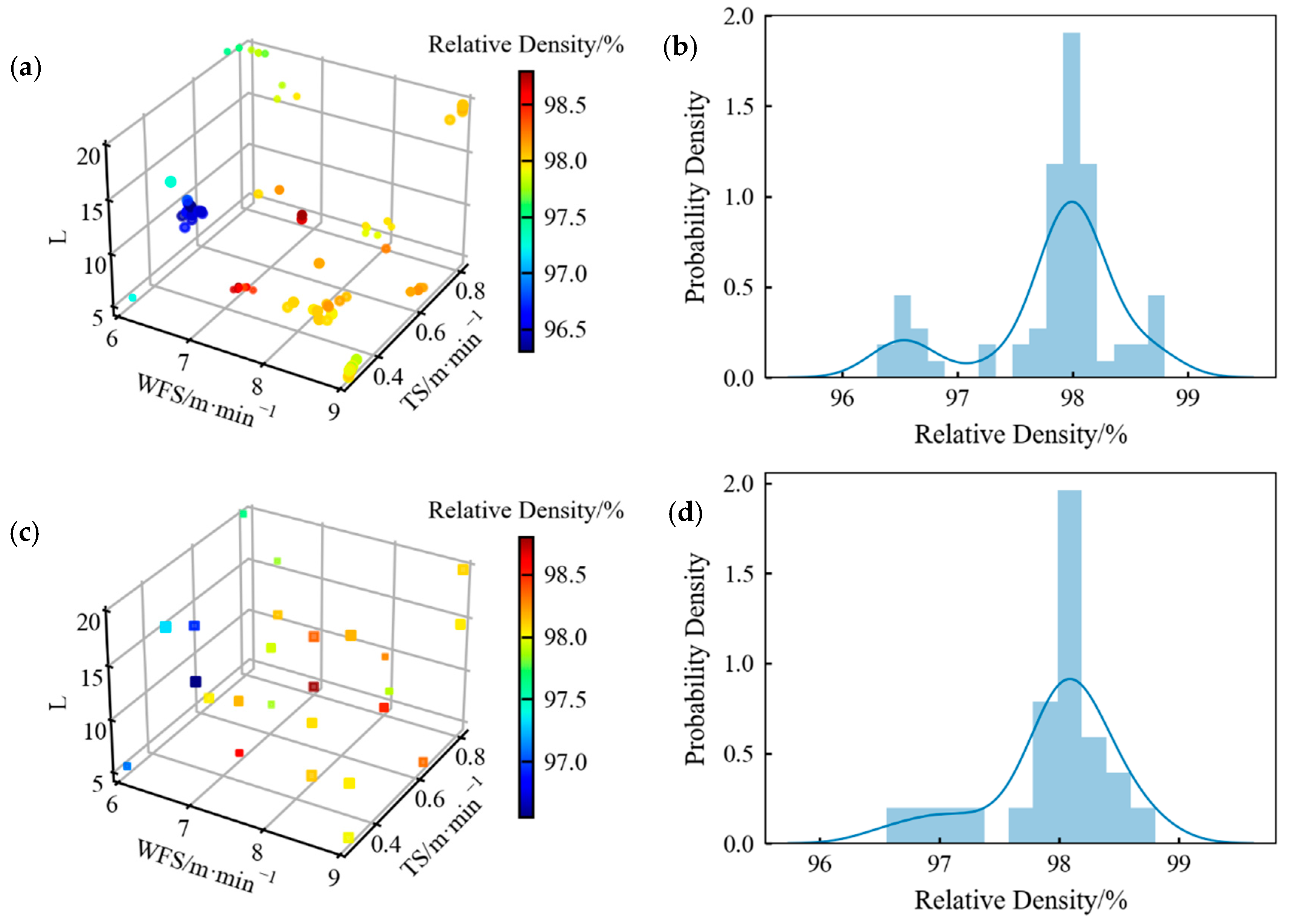
Figure 7 shows the distribution of 75 sets of generated data using the WGAN-GP method and 25 training sets obtained from the experiment. It can be seen that the generated data have a similar distribution to the real data. Based on the similarity ranking of the hybrid data, the performance of the models on the test set were examined by adding different amounts of generated data to the training set. The results show that the model performs best on the test set when the generated data/real data = 1:1 in the training set.
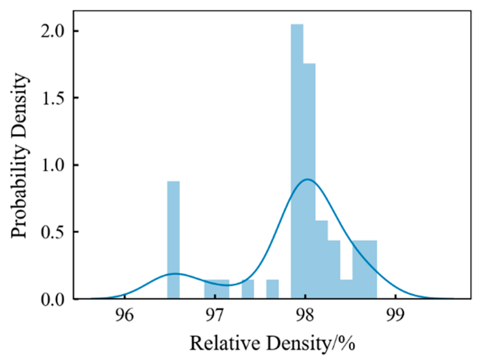
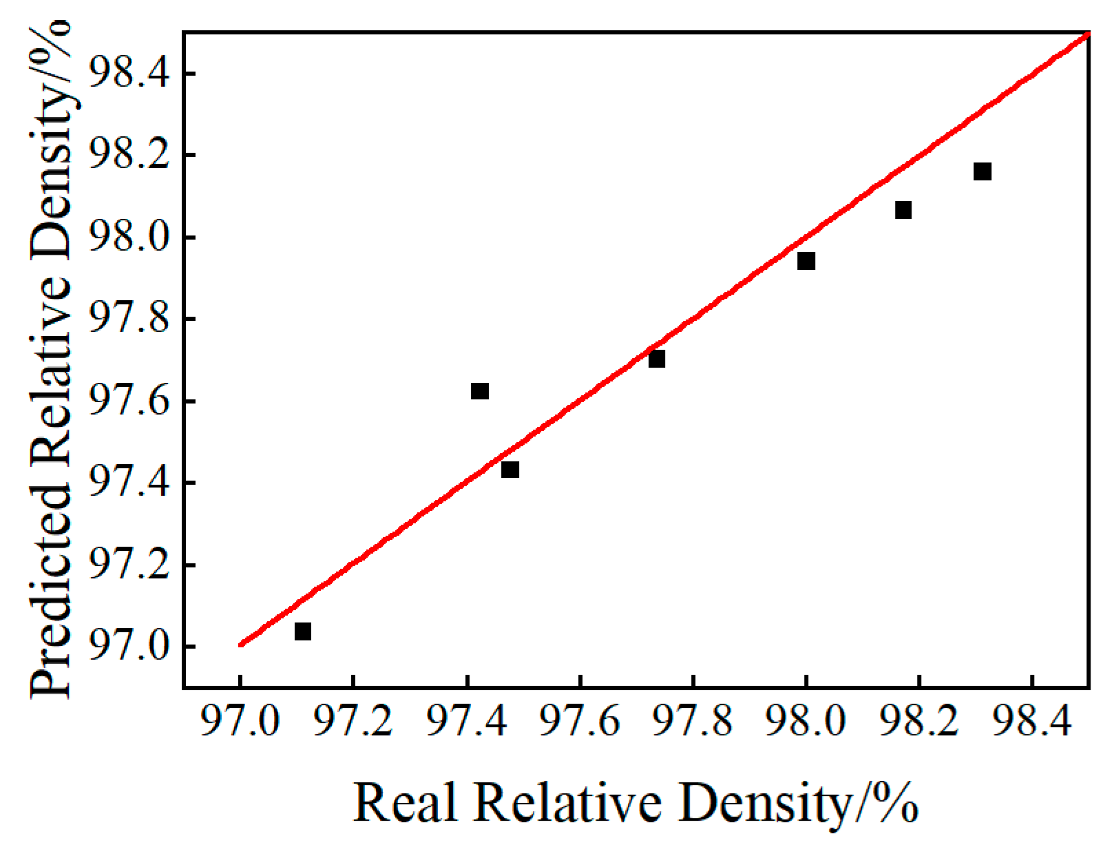
The performance of the models on the test set in the three cases of whether the data in the training set were augmented and whether the data were augmented with a similarity ranking is compared in Table 6. It demonstrates that the model with data augmentation and a similarity ranking of the data in the training set performs the best on the test set, with an R2 = 0.924, and MAE = 0.096. Figure 8 shows the probability density map of the relative density distribution of the hybrid data set corresponding to the best model. The distribution of the relative density in the mixed training set of the best model is similar to that in the training set consisting only of real data. Figure 9 shows the difference between the experimental values of the relative density on the test set and calculated values by the best model. The solid red line in the graph indicates that the calculated values are equal to the experimental values. As can be seen from Figure 9, the difference between the calculated values and the actual values is small, which is consistent with the results in Table 6.

3.3. High Relative Density Process Window Reliability Verification

The result of the range analysis suggests that the L has a greater impact on the relative density, with a range of 0.64, and the change in the TLW has a smaller impact on the relative density, with a range of only 0.03. Therefore, the changes in the process parameters window for a high relative density with different Ls have been analyzed. Figure 10 shows the relative densities calculated using the model when the TLW is 80 mm, and when the L, WFS, TS, and ICT are varied between 5–20 layers, 6–9 m·min−1, 0.3–0.798 m·min−1, and 60–180 s, respectively.
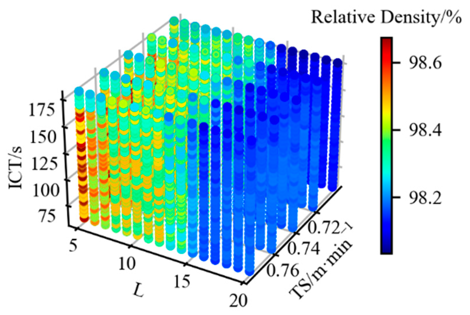
The relative densities of the samples increase with the increase in the TS. When the L is between 5 and 7, the TS window with a high relative density is 0.4–0.798 m·min−1, and when the L is larger than 7, it is 0.72–0.798 m·min−1. The relative density first increases and then decreases with an increase in the WFS. When the L is less than or equal to 15, the WFS window with a high relative density is 7–7.5 m·min−1, and when the L is larger than 15, the WFS window with a high relative density is 7.1~8 m·min−1. Although the generated data enhance the generalization performance of the model, there is still a limitation in the distribution of the data to maintain the similarity with the experimental data. This makes it so that there is no relative density greater than 98.5% with the model calculations when the L is larger than 15. In addition, when the L is less than or equal to 15, the relative density at a WFS between 7.5–8 m·min−1 is second only to that between 7–7.5 m·min−1 and is higher than at other WFS intervals. When the L increases, the relative density decreases first, and the relative density is the smallest at 16 layers. Then, it increases with an increase in the L. From the result of the range analysis, it is known that the effect of the ICT on the relative density is smaller than those of the WFS and TS, which makes the change in the relative density with the ICT in Figure 10b not show an obvious demarcation line. In order to further study the ICT window change, the relative density calculated using the model was visualized, where the WFS and TS are in the range of 7–8 m·min−1 and 0.72–0.798 m·min−1, respectively. The results are shown in Figure 11. As can be seen from Figure 11, the relative density change with the ICT is roughly bounded by 156 s. Although the relative density fluctuates greatly under the influence of the WFS and TS when the ICT is less than 156 s, the overall performance is still higher than when the ICT is greater than 156 s.
The process parameter windows corresponding to the 20-layer samples obtained above are listed in Table 7. In order to verify the validity of the obtained process windows, three 20-layer samples with a TLW of 100 mm were fabricated by selecting three groups of parameters in the windows of Table 7. The relative density and the mechanical properties of the specimens were tested. The results are summarized in Table 8. Figure 12a shows the engineering stress–engineering strain curves of the three tensile specimens. Due to Portevin–Le Chatelier (PLC) effect, the engineering stress–engineering strain curves of the three samples all show serrated characteristics. The interaction between the moving dislocation and the atoms of the diffused solute are thought to be the main cause of the PLC effect [34]. This appears in Al–Cu alloys as a moving dislocation in the α-Al matrix phase interacting with solute Cu atoms [9,35].
In the uniform plastic deformation stage, the relationship among the true stress (σT), true strain (εT), engineering stress (σE), and engineering strain (εE) can be expressed as:
σ T = σ E ( 1 + ε E )
ε T = ln ( 1 + ε E )
Figure 12b shows the true stress–true strain curves before necking begins. In addition, the Hollomon equation is satisfied between the true stress and the true strain, which is expressed as follows [9]:
σ T = K ε T n
where K is the strength coefficient, and n is the strain-hardening exponent. A logarithmic transformation of Equation (16) gives the following equation:
ln σ T = n ln ε T + ln K
Figure 12c shows the lnσT–lnεT relationship curves. The n values of different samples were obtained by fitting the lnσT–lnεT curves. In general, a higher n value means that the material is able to achieve sufficient work hardening in critical areas, and the material has a better formability [36]. As can be seen from Figure 12c, the n value S3 is the largest, which is 0.266. Additionally, the size of the n value corresponds to the elongation (εef).
Due to the small size of the data set and the low repeatability of the metal additive manufacturing process, the relative densities of the three samples in the verification experiment are higher than the relative density calculated using the model in Figure 10. The maximum value of the relative densities in the verification experiment can reach 98.77%. That is, the porosity is 1.23%, which is better than the porosity (1.52%) obtained by using the percentage of the area from the statistics of Fang et al. [37]. The ultimate tensile strength (UTS) can reach 279.96 MPa, which is better than the 274 MPa proposed by Fang et al. [38], and the yield strength is all greater than 110 MPa, indicating that the process window obtained from the proposed model can produce the thin-walled components of the WAAM 2219 aluminum alloy with a higher relative density and better mechanical properties.

4. Conclusions

In this research, we studied the influences of different dimension parameters and process parameters on the relative density of 2219 aluminum alloy thin-walled components manufactured using WAAM. And the relationship among the process parameters, dimensional parameters, and relative density was modeled on the basis of the experimental data combined with the data augmentation method. In addition, variations of the high relative density process window were investigated based on the obtained relationship model, and the obtained process window was experimentally verified.
The results show that the influence of each parameter on the relative density is in the following order: TS > WFS > L > ICT > TLW. The relative density of the sample increased first, and then decreased with an increase in the WFS and increased with an increase in the TS. When the WFS was 6 m·min−1, the relative density of the sample was smaller than when the WFS was 9 m·min−1. When the L increased, the relative density of the sample first decreased and then increased. In addition, an excessive ICT would reduce the relative density, while the TLW had little effect on the relative density. When the heat input of the sample was not large and the cooling rate of the molten pool was high, the pore defects in the sample were mainly unfused defects. Data augmentation of the experimentally obtained small data set can effectively improve the generalization performance of the proposed parameter–relative density relationship model. With the change in the L, the process window of the WFS changed at 15 layers and the process window of the TS changed at 7 layers, but the process window of the ICT did not change significantly. The relative density of the specimens in the validation experiment can reach 98.77%, and the UTS can reach 279.96 Mpa.
This work can provide some guidance in the selection of process parameters for WAAM aluminum alloy components. Future work will carry out high-throughput experiments to obtain larger data sets for modeling, in order to achieve the goal of reducing the error caused by a low repeatability of the manufacturing process and improving the accuracy of the model.

Author Contributions

W.G. and B.L.: conceptualization and funding acquisition; Y.W. (Yajun Wu), Z.L. and Y.W. (Yuzhong Wang): writing—original draft and investigation; Y.W. (Yajun Wu): analyzing, modeling, and visualization; W.G., Y.W. (Yajun Wu), Z.L. and Y.W. (Yuzhong Wang): writing, review, and editing. All authors have read and agreed to the published version of the manuscript.

Funding

This work was financially supported by the National Key Research and Development Program of China [grant number 2021YFB1715600].

Data Availability Statement

The original contributions presented in the study are included in the article, further inquiries can be directed to the corresponding author.

Acknowledgments

This work was supported by the National Innovation Institute of Additive Manufacturing, China.

Conflicts of Interest

The authors declare no conflicts of interest.

References

  1. Kumar Sinha, A.; Pramanik, S.; Yagati, K.P. Research Progress in Arc Based Additive Manufacturing of Aluminium Alloys—A Review. Measurement 2022, 200, 111672. [Google Scholar] [CrossRef]
  2. Bartsch, H.; Kühne, R.; Citarelli, S.; Schaffrath, S.; Feldmann, M. Fatigue Analysis of Wire Arc Additive Manufactured (3D Printed) Components with Unmilled Surface. Structures 2021, 31, 576–589. [Google Scholar] [CrossRef]
  3. Vishnukumar, M.; Pramod, R.; Rajesh Kannan, A. Wire Arc Additive Manufacturing for Repairing Aluminium Structures in Marine Applications. Mater. Lett. 2021, 299, 130112. [Google Scholar] [CrossRef]
  4. Bermingham, M.J.; Nicastro, L.; Kent, D.; Chen, Y.; Dargusch, M.S. Optimising the Mechanical Properties of Ti-6Al-4V Components Produced by Wire + Arc Additive Manufacturing with Post-Process Heat Treatments. J. Alloys Compd. 2018, 753, 247–255. [Google Scholar] [CrossRef]
  5. Wu, B.; Pan, Z.; Ding, D.; Cuiuri, D.; Li, H.; Xu, J.; Norrish, J. A Review of the Wire Arc Additive Manufacturing of Metals: Properties, Defects and Quality Improvement. J. Manuf. Process. 2018, 35, 127–139. [Google Scholar] [CrossRef]
  6. Li, Q.; Wu, A.; Li, Y.; Wang, G.; Yan, D.; Liu, J. Influence of Temperature Cycles on the Microstructures and Mechanical Properties of the Partially Melted Zone in the Fusion Welded Joints of 2219 Aluminum Alloy. Mater. Sci. Eng. A 2015, 623, 38–48. [Google Scholar] [CrossRef]
  7. Zhou, Y.; Lin, X.; Kang, N.; Huang, W.; Wang, J.; Wang, Z. Influence of Travel Speed on Microstructure and Mechanical Properties of Wire + Arc Additively Manufactured 2219 Aluminum Alloy. J. Mater. Sci. Technol. 2020, 37, 143–153. [Google Scholar] [CrossRef]
  8. Hu, Y.; Deng, X.; Kan, Q.; Wu, S.; Li, Y.; Lei, L.; Wang, L.; Kang, G. Influence of Temperature on Deformation and Damage Mechanisms of Wire + Arc Additively Manufactured 2219 Aluminum Alloy. Eng. Fract. Mech. 2023, 292, 109675. [Google Scholar] [CrossRef]
  9. Wang, Z.; Lin, X.; Wang, L.; Cao, Y.; Zhou, Y.; Huang, W. Microstructure Evolution and Mechanical Properties of the Wire + Arc Additive Manufacturing Al-Cu Alloy. Addit. Manuf. 2021, 47, 102298. [Google Scholar] [CrossRef]
  10. Gu, J.; Gao, M.; Yang, S.; Bai, J.; Ding, J.; Fang, X. Pore Formation and Evolution in Wire + Arc Additively Manufactured 2319 Al Alloy. Addit. Manuf. 2019, 30, 100900. [Google Scholar] [CrossRef]
  11. Li, Q.; Feng, C.; Liu, B.; Zhou, Q.; Hu, W.; Wang, F. Influence of WAAM Process Parameters on Micro Porosities of Additively Manufactured 2219Aluminum Alloy. Aerosp. Mater. Technol. 2022, 52, 129–133. [Google Scholar]
  12. Ryan, E.M.; Sabin, T.J.; Watts, J.F.; Whiting, M.J. The Influence of Build Parameters and Wire Batch on Porosity of Wire and Arc Additive Manufactured Aluminium Alloy 2319. J. Mater. Process. Technol. 2018, 262, 577–584. [Google Scholar] [CrossRef]
  13. Hauser, T.; Reisch, R.T.; Breese, P.P.; Lutz, B.S.; Pantano, M.; Nalam, Y.; Bela, K.; Kamps, T.; Volpp, J.; Kaplan, A.F.H. Porosity in Wire Arc Additive Manufacturing of Aluminium Alloys. Addit. Manuf. 2021, 41, 101993. [Google Scholar] [CrossRef]
  14. Derekar, K.; Lawrence, J.; Melton, G.; Addison, A.; Zhang, X.; Xu, L. Influence of Interpass Temperature on Wire Arc Additive Manufacturing (WAAM) of Aluminium Alloy Components. MATEC Web Conf. 2019, 269, 05001. [Google Scholar] [CrossRef]
  15. Le, V.T.; Mai, D.S.; Doan, T.K.; Paris, H. Wire and Arc Additive Manufacturing of 308L Stainless Steel Components: Optimization of Processing Parameters and Material Properties. Eng. Sci. Technol. Int. J. 2021, 24, 1015–1026. [Google Scholar] [CrossRef]
  16. Naveen Srinivas, M.; Vimal, K.E.K.; Manikandan, N.; Sritharanandh, G. Parametric Optimization and Multiple Regression Modelling for Fabrication of Aluminium Alloy Thin Plate Using Wire Arc Additive Manufacturing. Int. J. Interact. Des. Manuf. IJIDeM 2022, 1–11. [Google Scholar] [CrossRef]
  17. Ni, M.; Zhou, Y.; Hu, Z.; Qin, X.; Xiong, X.; Ji, F. Forming Optimization for WAAM with Weaving Deposition on Curved Surfaces. Int. J. Mech. Sci. 2023, 252, 108366. [Google Scholar] [CrossRef]
  18. Ouyang, J.; Li, M.; Lian, Y.; Peng, S.; Liu, C. A Fast Prediction Model for Liquid Metal Transfer Modes during the Wire Arc Additive Manufacturing Process. Materials 2023, 16, 2911. [Google Scholar] [CrossRef]
  19. Singh Sivam Sundarlingam Paramasivam, S.; Damodar Sawant, L.; Natarajan, H.; Sumanth, U.; Pratap Singh, K. Numerical Simulation Process Parameter Optimization in Metal Additive Manufacturing for Getting Better Quality of Products. Mater. Today Proc. 2022, 66, 850–857. [Google Scholar] [CrossRef]
  20. Xiao, X.; Waddell, C.; Hamilton, C.; Xiao, H. Quality Prediction and Control in Wire Arc Additive Manufacturing via Novel Machine Learning Framework. Micromachines 2022, 13, 137. [Google Scholar] [CrossRef]
  21. Dharmawan, A.G.; Xiong, Y.; Foong, S.; Song Soh, G. A Model-Based Reinforcement Learning and Correction Framework for Process Control of Robotic Wire Arc Additive Manufacturing. In Proceedings of the 2020 IEEE International Conference on Robotics and Automation (ICRA), Paris, France, 31 May–31 August 2020; pp. 4030–4036. [Google Scholar] [CrossRef]
  22. Ling, Y.; Ni, J.; Antonissen, J.; Ben Hamouda, H.; Vande Voorde, J.; Abdel Wahab, M. Numerical Prediction of Microstructure and Hardness for Low Carbon Steel Wire Arc Additive Manufacturing Components. Simul. Model. Pract. Theory 2023, 122, 102664. [Google Scholar] [CrossRef]
  23. Tapia, G.; Elwany, A.H.; Sang, H. Prediction of Porosity in Metal-Based Additive Manufacturing Using Spatial Gaussian Process Models. Addit. Manuf. 2016, 12, 282–290. [Google Scholar] [CrossRef]
  24. Liu, Q.; Wu, H.; Paul, M.J.; He, P.; Peng, Z.; Gludovatz, B.; Kruzic, J.J.; Wang, C.H.; Li, X. Machine-Learning Assisted Laser Powder Bed Fusion Process Optimization for AlSi10Mg: New Microstructure Description Indices and Fracture Mechanisms. Acta Mater. 2020, 201, 316–328. [Google Scholar] [CrossRef]
  25. GB/T 3850-2015; Impermeable Sintered Metal Materials and Hardmetals—Determination of Density. General Administration of Quality Supervision, Inspection and Quarantine of the People’s Republic of China; Standardization Administration of the People’s Republic of China: Beijing, China, 2015.
  26. Chen, T.; Guestrin, C. XGBoost: A Scalable Tree Boosting System. In Proceedings of the 22nd ACM SIGKDD International Conference on Knowledge Discovery and Data Mining, San Francisco, CA, USA, 13–17 August 2016; pp. 785–794. [Google Scholar] [CrossRef]
  27. Pan, B. Application of XGBoost Algorithm in Hourly PM2.5 Concentration Prediction. IOP Conf. Ser. Earth Environ. Sci. 2018, 113, 012127. [Google Scholar] [CrossRef]
  28. Ding, P. Modeling Method for Complex Industrial Process Based on GANs Data Augmentation. Master’s Thesis, China University of Mining and Technology, Xuzhou, China, 2021. Available online: https://kns.cnki.net/KCMS/detail/detail.aspx?dbcode=CMFD&dbname=CMFD202201&filename=1021774558.nh&v= (accessed on 18 February 2023).
  29. Fu, W.; Zhang, D.; Fu, Y.; Li, J.; Xie, Y. Arrears Prediction for Electricity Customer through Wgan-Gp. In Proceedings of the 2017 IEEE 2nd Information Technology, Networking, Electronic and Automation Control Conference (ITNEC), Chengdu, China, 15–17 December 2017; IEEE: Chengdu, China, 2017; pp. 1667–1670. [Google Scholar] [CrossRef]
  30. Cong, B.; Ouyang, R.; Qi, B.; Ding, J. Influence of Cold Metal Transfer Process and Its Heat Input on Weld Bead Geometry and Porosity of Aluminum-Copper Alloy Welds. Rare Met. Mater. Eng. 2016, 45, 606–611. [Google Scholar] [CrossRef]
  31. Sanaei, N.; Fatemi, A.; Phan, N. Defect Characteristics and Analysis of Their Variability in Metal L-PBF Additive Manufacturing. Mater. Des. 2019, 182, 108091. [Google Scholar] [CrossRef]
  32. Wu, S.; Hu, Y.; Yang, B.; Zhang, H.; Guo, G.; Kang, G. Review on Defect Characterization and Structural Integrity Assessment Method of Additively Manufactured Materials. J. Mech. Eng. 2021, 57, 3–34. [Google Scholar]
  33. Jiang, G.; Liu, Y.; Li, Y.; Su, Y.; Guo, J. A model for calculating solubility of hydrogen in molten aluminum alloys. Acta Metall. Sin. 2008, 44, 129–133. [Google Scholar]
  34. Hsu, W.-C.; Shen, T.-E.; Liang, Y.-C.; Yeh, J.-W.; Tsai, C.-W. In Situ Analysis of the Portevin-Le Chatelier Effect from Low to High-Entropy Alloy in Equal HfNbTaTiZr System. Acta Mater. 2023, 253, 118981. [Google Scholar] [CrossRef]
  35. Nie, X.; Zhang, H.; Zhu, H.; Hu, Z.; Qi, Y.; Zeng, X. On the Role of Zr Content into Portevin-Le Chatelier (PLC) Effect of Selective Laser Melted High Strength Al-Cu-Mg-Mn Alloy. Mater. Lett. 2019, 248, 5–7. [Google Scholar] [CrossRef]
  36. Uijl, N.J.D.; Carless, L.J. Advanced Metal-Forming Technologies for Automotive Applications. In Advanced Materials in Automotive Engineering; Woodhead Publishing: Sawston, UK, 2012; pp. 28–56. [Google Scholar] [CrossRef]
  37. Fang, X.; Zhang, L.; Li, H.; Li, C.; Huang, K.; Lu, B. Microstructure Evolution and Mechanical Behavior of 2219 Aluminum Alloys Additively Fabricated by the Cold Metal Transfer Process. Materials 2018, 11, 812. [Google Scholar] [CrossRef] [PubMed]
  38. Fang, Y.; Wang, L.; Sun, L.; Lyu, F.; Zhang, J.; Zhan, X. Influence of Heat Flow on the Grain Morphology and Porosity of Wire Arc Additive Manufactured 2319 Aluminum Alloy. Met. Mater. Int. 2023, 1–13. [Google Scholar] [CrossRef]
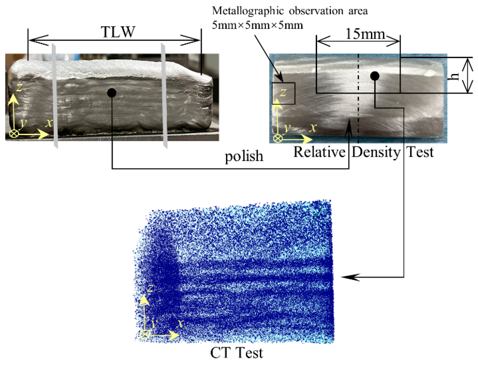
Figure 1. Relative density, CT test, and optical microscope observation area.
Metals 14 00330 g001
Figure 2. Tensile samples. (a) The position of tensile samples, (b) the size of tensile samples.
Metals 14 00330 g002
Figure 3. WGAN-GP structures.
Metals 14 00330 g003
Figure 4. The optical microscope images.
Metals 14 00330 g004
Figure 5. The projected area distribution of pore defects on the spatial reference plane: (a) sample 26, HI = 144.79 J·mm−1; (b) sample 27, HI = 445.54 J·mm−1; (c) sample 1, HI = 385.15 J·mm−1; (d) sample 17, HI = 246.90 J·mm−1.
Metals 14 00330 g005
Figure 6. Relative density variations with process parameters: (a) WFS, (b) TS, (c) L, (d) ICT, and (e) TLW.
Metals 14 00330 g006
Figure 7. Generated data vs. real data distribution. (a) Spatial distribution of generated data. (b) Probability density distribution of the generated relative density. (c) Spatial distribution of real data. (d) Probability density distribution of the real relative density. The size of the dots in (a,c) indicates the size of the ICT, and the transparency represents the size of the TLW.
Metals 14 00330 g007
Figure 8. The best model corresponds to the relative density probability distribution of the training set.
Metals 14 00330 g008
Figure 9. Performance of the best model on the test set.
Metals 14 00330 g009
Figure 10. Process window variation with L: (a,b) visualization of WFS and TS windows, and (c) ICT window visualization. The size of the dots in (a,b) indicates the size of the ICT, and the size of the dots in (c) indicates the size of the WFS.
Metals 14 00330 g010
Figure 11. Visualization of ICT window at WFS in the range of 7–8 m·min−1 and TS in the range of 0.72–0.798 m·min−1. The size of the dots indicates the size of WFS.
Metals 14 00330 g011
Figure 12. (a) Engineering stress–strain curves; (b) true stress (σT)–true strain curves (εT); (c) lnσT–lnεT curves. The dashed lines in (c) represent the fitting curves of lnεT and lnσT, which is the same color as the solid line and represents different samples.
Metals 14 00330 g012
Table 1. Composition of GR-2319 (wt %).
SiFeCuMnMgZnTiVZrAl
0.20.35.8–6.80.20–0.400.020.100.1–0.20.05–0.150.1–0.25other
Table 2. Processing parameters.
ParametersLevel
1234
WFS/m·min−16789
TS/m·min−10.3000.4680.6360.798
L5101520
ICT/s60120150180
TLW/mm6080//
Table 3. WGAN-GP architecture.
Network LayerNumber of KernelKernel SizeOutput SizeActivation FunctionD/G
Fully connected layer//(None, 6)reluG
Reshape layer//(None, 6, 1)/
1D convolutional layer323(None, 6, 32)relu
1D convolutional layer13(None, 6, 1)tanh
Input layer//(None, 6, 1)/D
1D convolutional layer323(None, 6, 32)leakyrelu
Flatten layer//(None, 192)/
Fully connected layer//(None, 64)/
Dropout layer//(None, 64)/
Fully connected layer//(None, 1)/
Table 4. The relative densities for different parameter combinations.
SampleWFS/m·min−1TS/m·min−1LICT/sTLW/mmRelative Density/%
160.3005606097.06
260.63651508098.02
370.4685606098.59
470.79851508098.80
580.46851808098.13
680.79851206098.49
790.30051808098.01
890.63651206098.35
960.300101208097.11
1060.636101806097.74
1170.468101208098.17
1270.798101806098.38
1380.468101506098.07
1480.79810608098.30
1590.300101506098.03
1690.63610608098.31
1760.468151806097.32
1860.798151208097.42
1970.300151806096.56
2070.636151208098.14
2180.30015608097.86
2280.636151506098.17
2390.46815608097.90
2490.798151506098.04
2560.468201508097.48
2660.79820606097.65
2770.300201508096.90
2870.63620606097.85
2980.300201206097.95
3080.636201808098.17
3190.468201206098.00
3290.798201808098.10
Table 5. Relative density range analysis.
FactorsWFS/m·min−1TS/m·min−1LICT/sTLW/mm
K1j779.806779.483785.452783.5171566.258
K2j783.374783.642784.103783.6401566.812
K3j785.151784.755781.414783.511/
K4j784.741785.191782.102782.403/
k1j97.47697.43598.18197.94097.891
k2j97.92297.95598.01397.95597.926
k3j98.14498.09497.67797.938/
k4j98.09398.14997.76397.800/
Original range (R)0.6680.7140.5040.1550.035
Range after conversion (R′)0.850.910.640.200.03
Table 6. Performance of the model on the test set, from the training set with or without data augmentation and similarity ranking.
Data EnhancementSimilarity OrderingMAER2
NoNo0.1380.816
YesNo0.1130.870
YesYes0.0960.924
Table 7. High relative density process window for 20-layer specimens.
Process ParametersLower LimitUpper Limit
WFS/m·min−17.18.0
TS/m·min−10.7200.798
ICT/s60156
Table 8. High relative density process window validation experiments.
SpecimenWFS
/m·min−1
TS
/m·min−1
ICT/sRelative
Density/%
UTS/MPaYS/MPaεef/%
S17.10.7209098.77267.76123.228.47
S27.50.7599098.49251.24129.527.18
S38.00.7989098.63279.96132.7711.43
Disclaimer/Publisher’s Note: The statements, opinions and data contained in all publications are solely those of the individual author(s) and contributor(s) and not of MDPI and/or the editor(s). MDPI and/or the editor(s) disclaim responsibility for any injury to people or property resulting from any ideas, methods, instructions or products referred to in the content.