
Modeling Metallic Fatigue Data Using the Birnbaum–Saunders Distribution

Abstract
:1. Introduction
2. Model Calibration and Comparison for Dataset 1
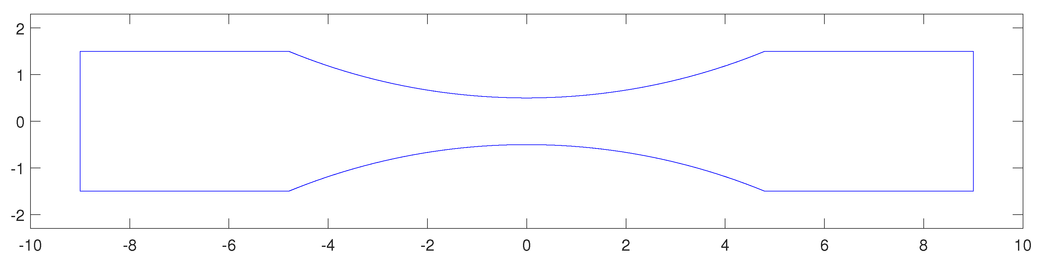
2.1. Description of Dataset 1
- Maximum stress, , measured in ksi units;
- Cycle ratio, R, defined as the minimum to maximum stress ratio. The ratio R is positive when the experiment corresponds to tension–tension loading and negative when the experiment corresponds to tension–compression loading;
- Fatigue-life, N, defined as the number of load cycles at which fatigue failure occurred; and
- A binary variable (0/1) to denote whether the test stopped before failure (run-out).
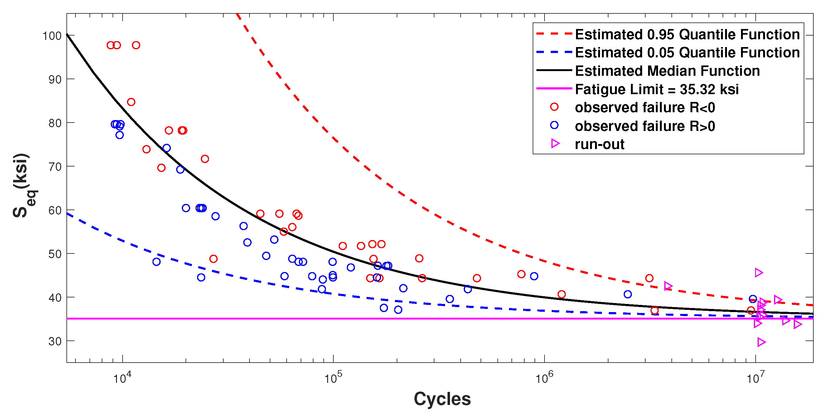
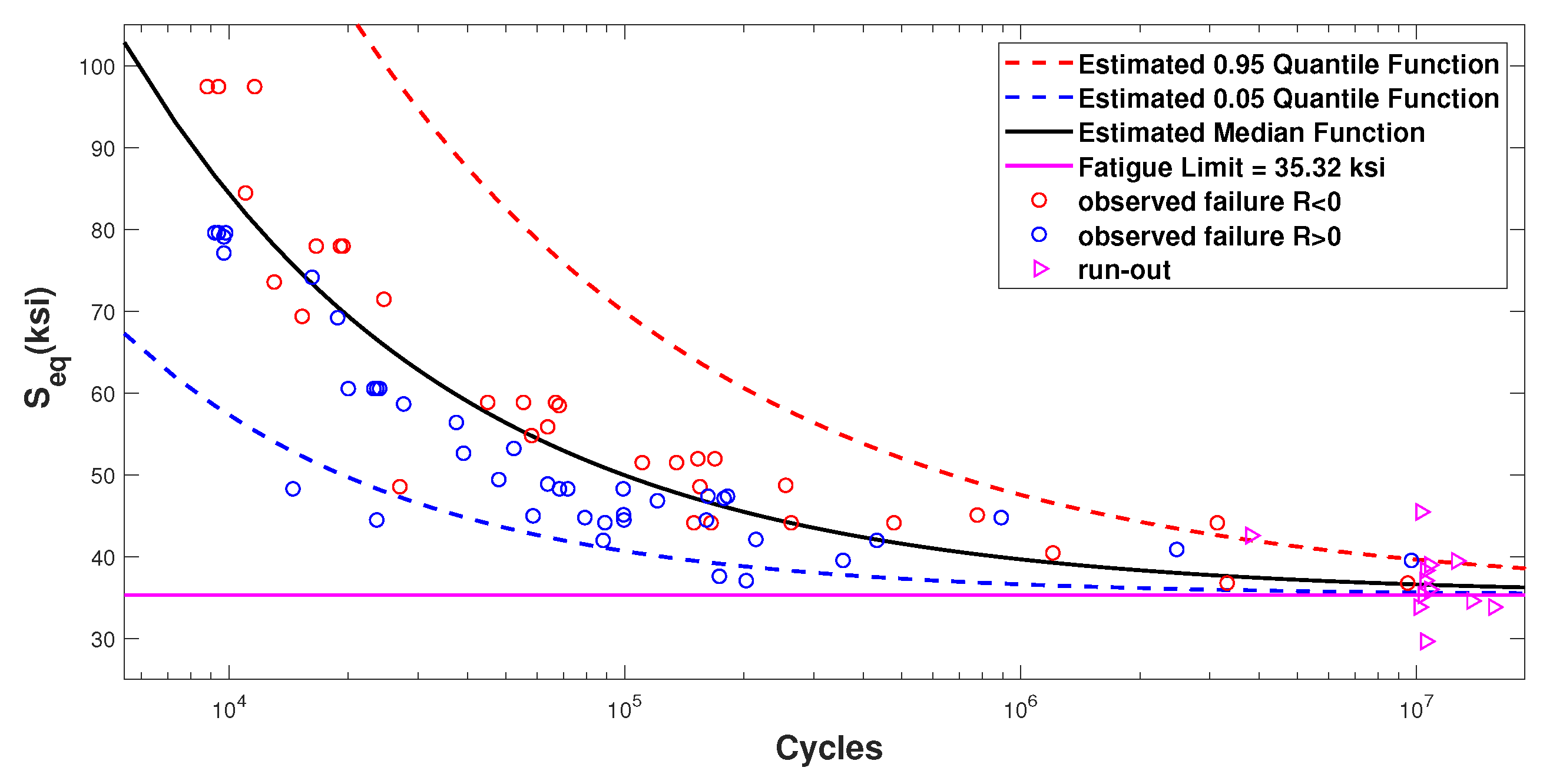
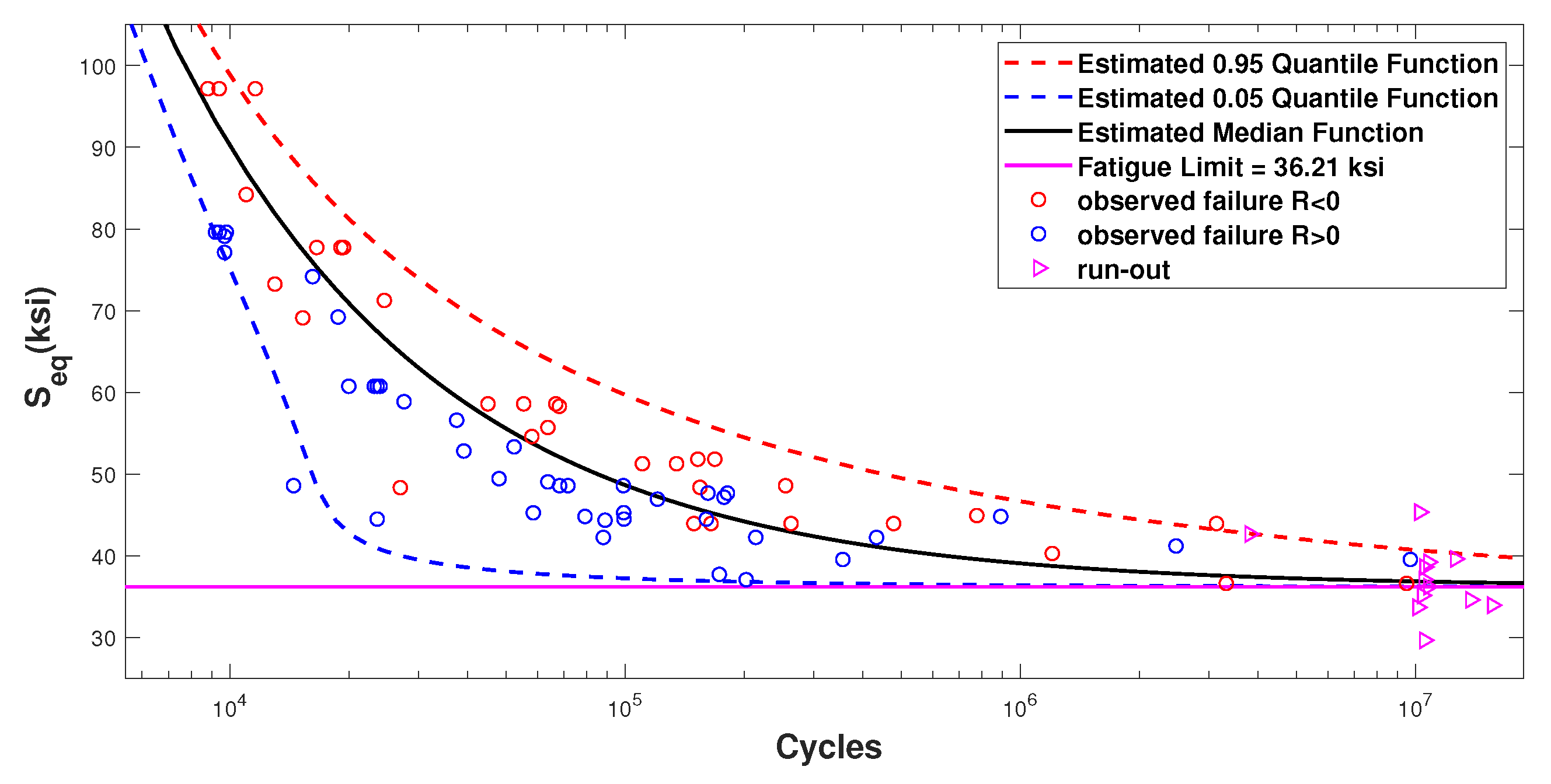
2.2. Fatigue-Limit Models
2.2.1. Model Ia
2.2.2. Model IIa
2.2.3. Model IIIa
2.2.4. Model Ib
2.2.5. Model IIb
2.2.6. Model IIIb
2.3. Model Comparison
3. Analysis of the Stress Ratio Effect and Equivalent Stress for Dataset 1
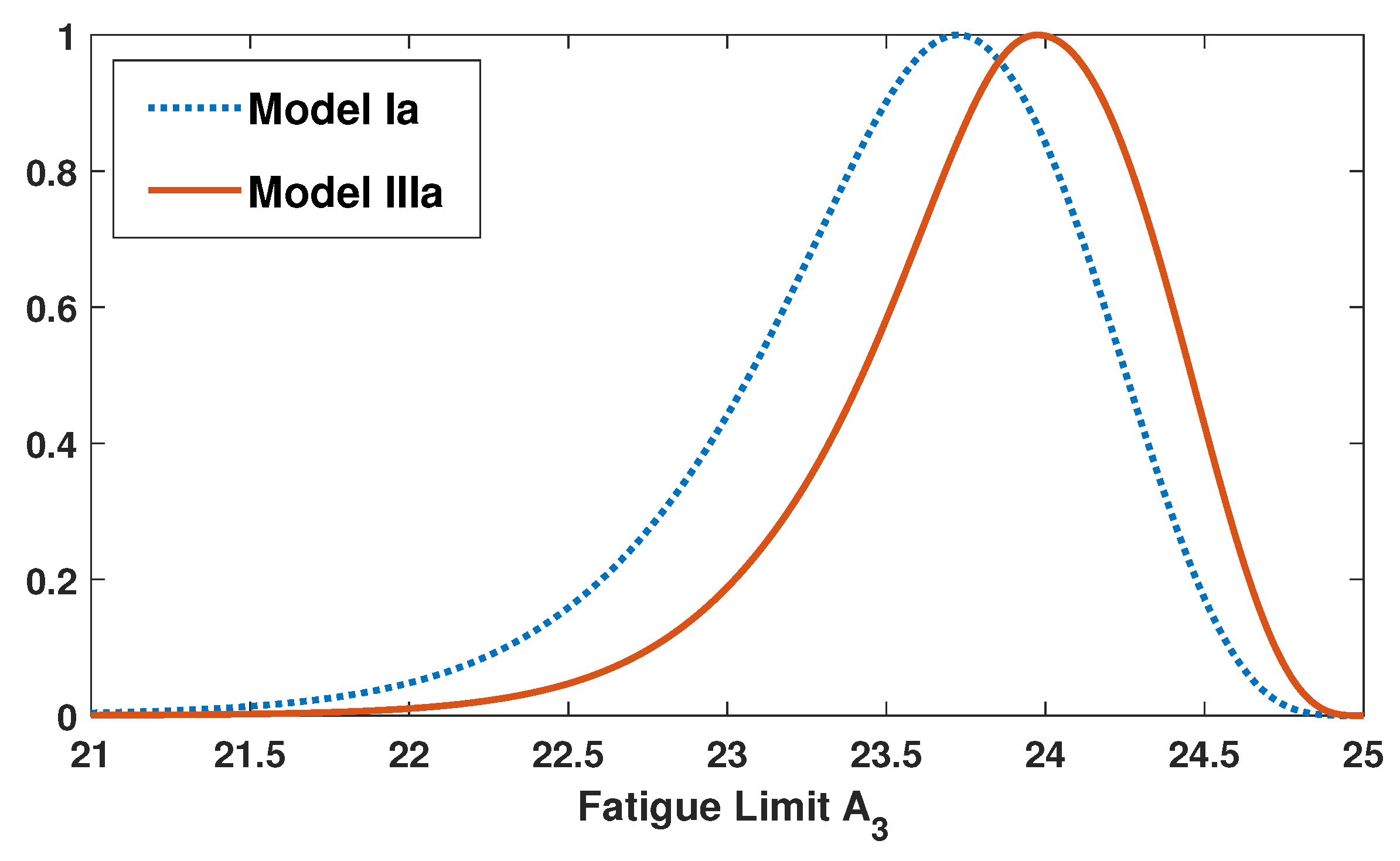
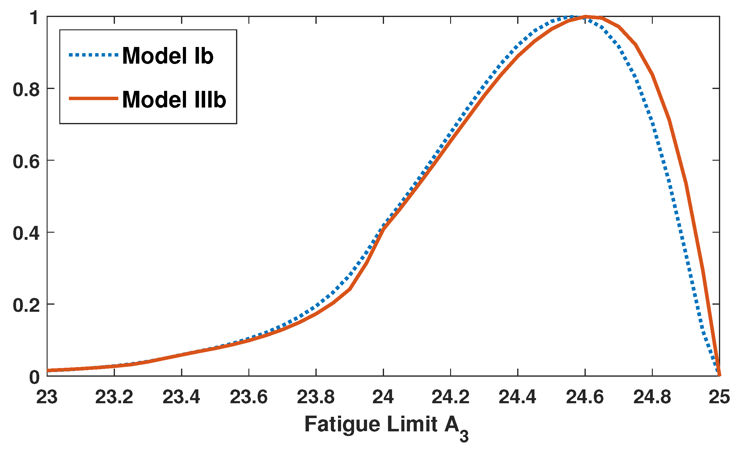
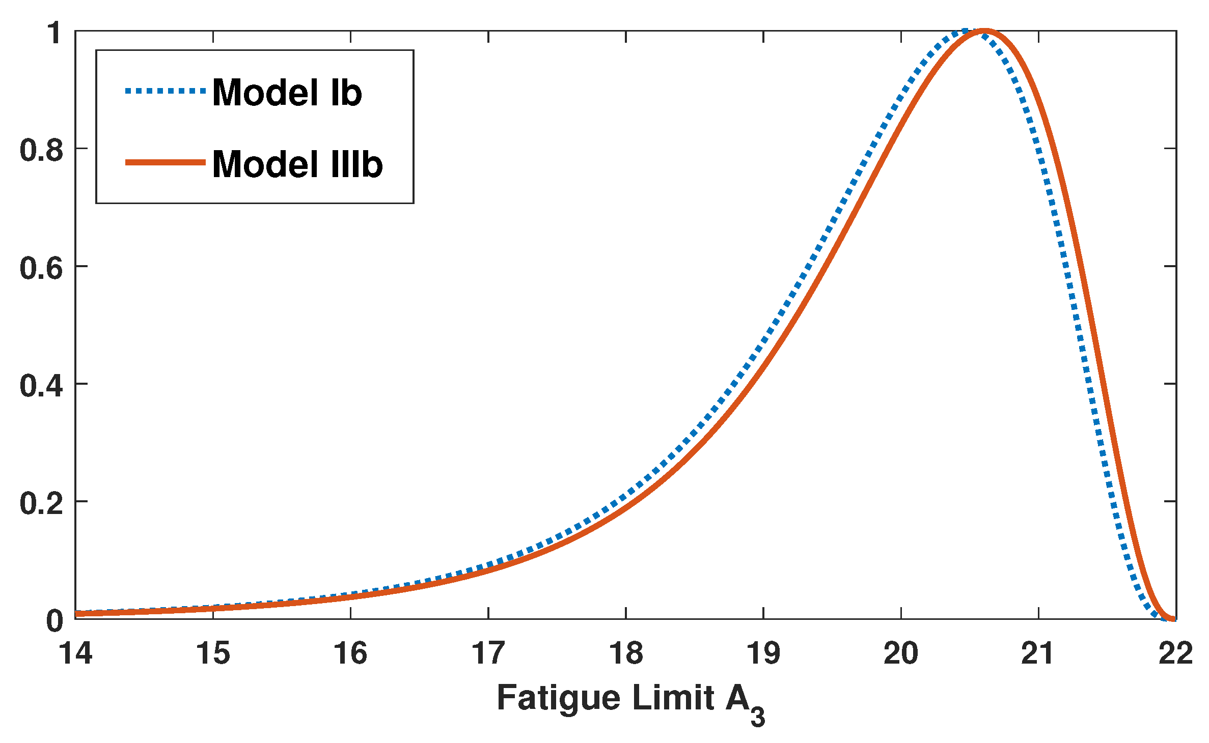
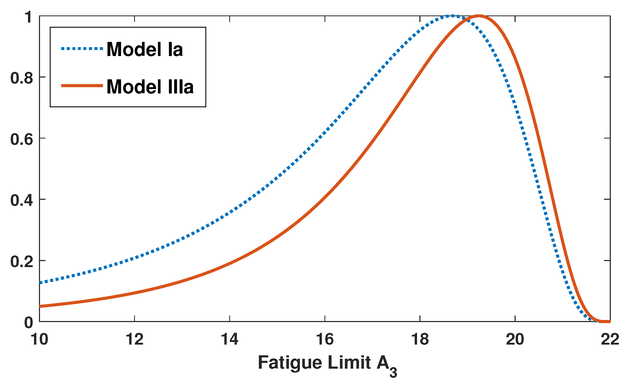
3.1. Profile Likelihood
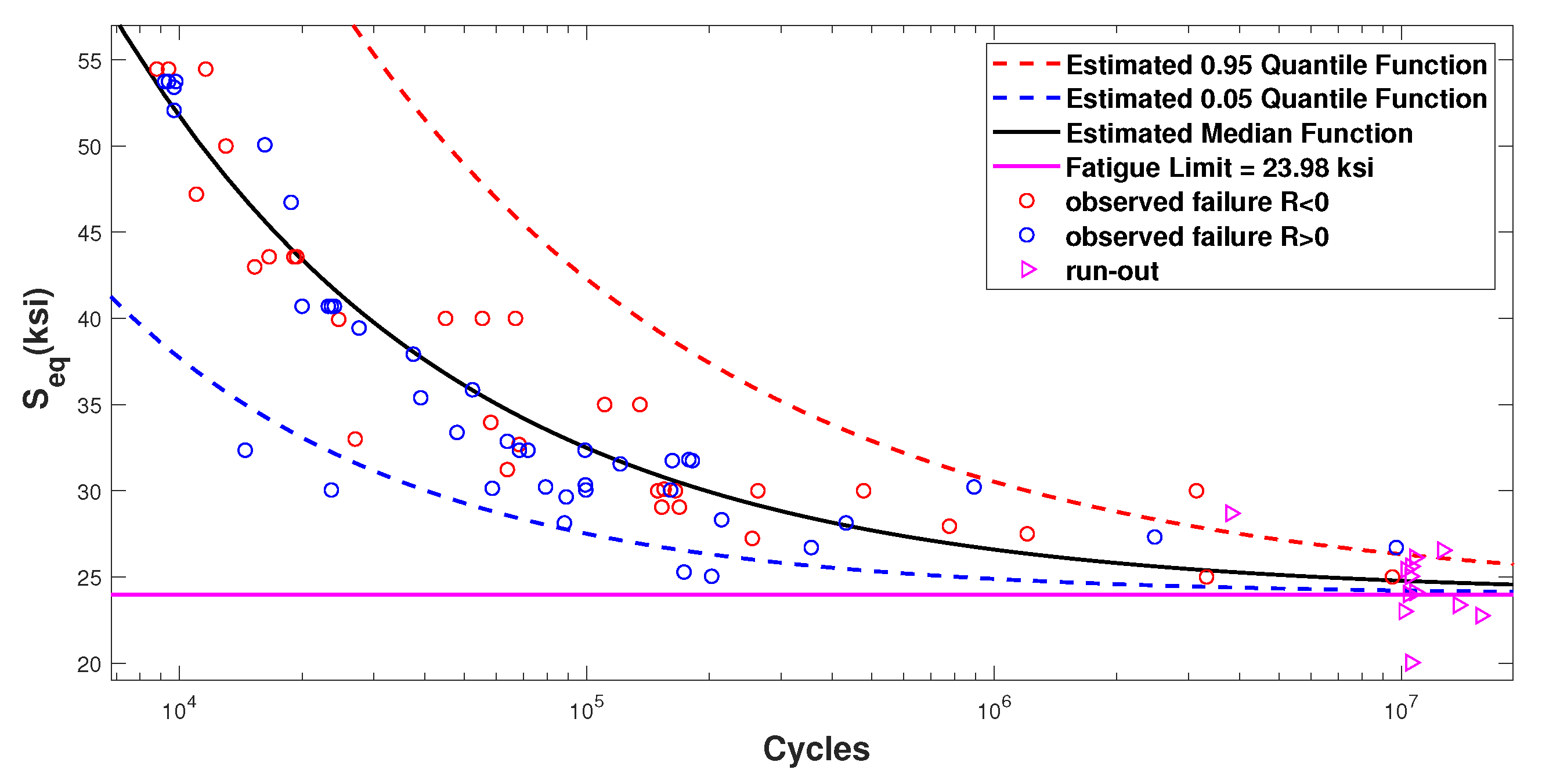
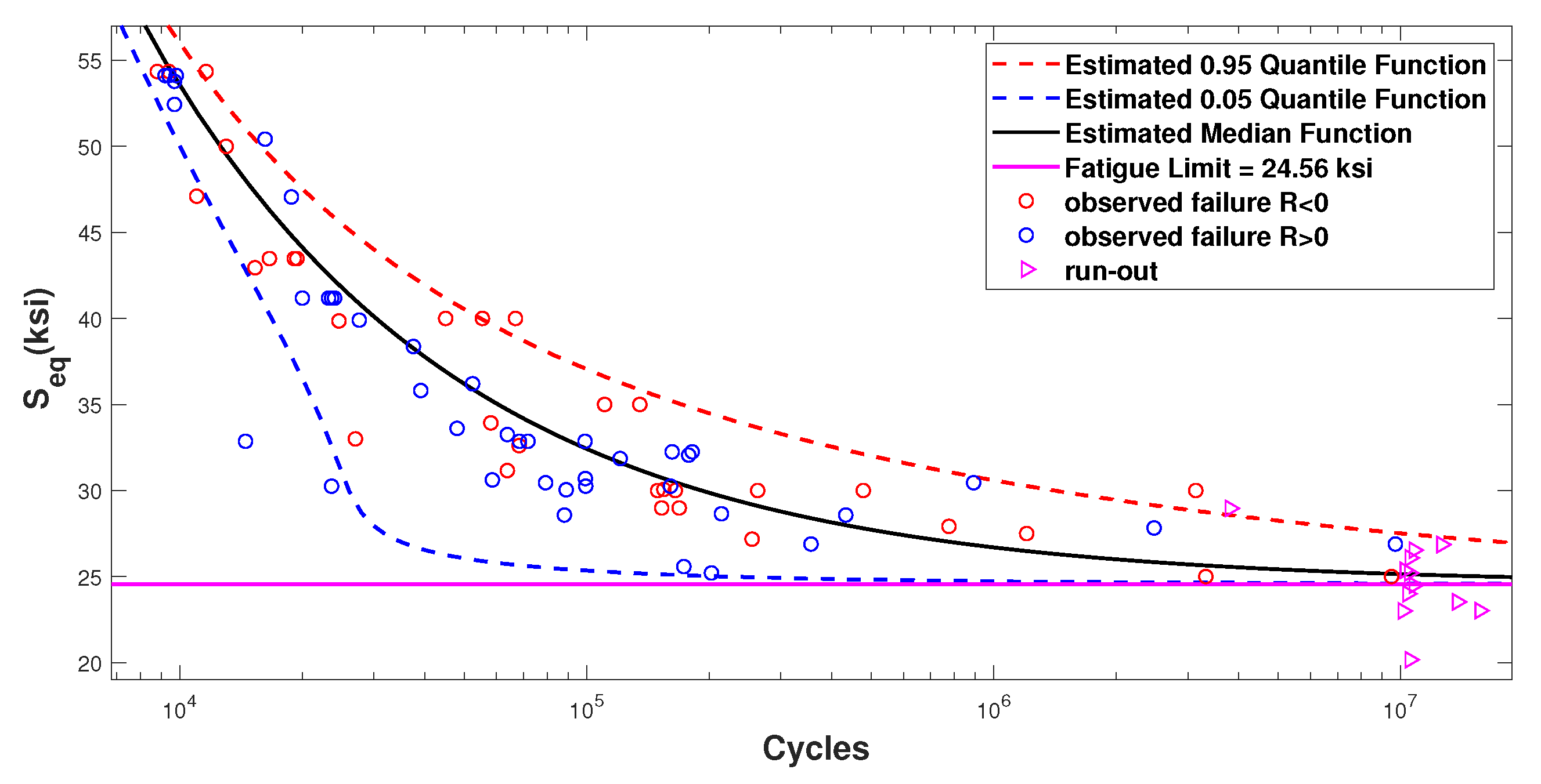
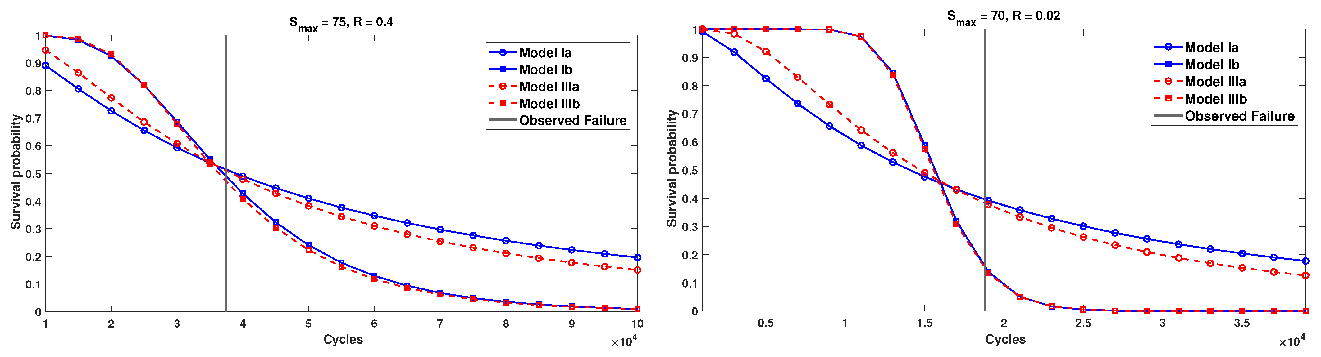
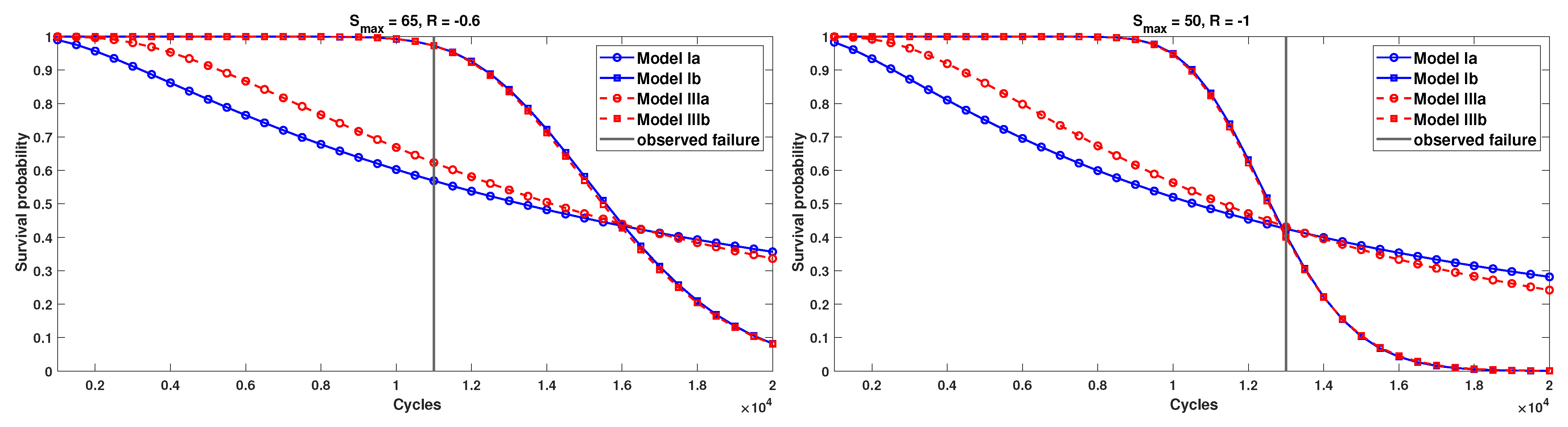
3.2. Survival Functions
4. Model Calibration and Comparison for Dataset 2
4.1. Description of Dataset 2
4.2. Profile Likelihood and Confidence Intervals
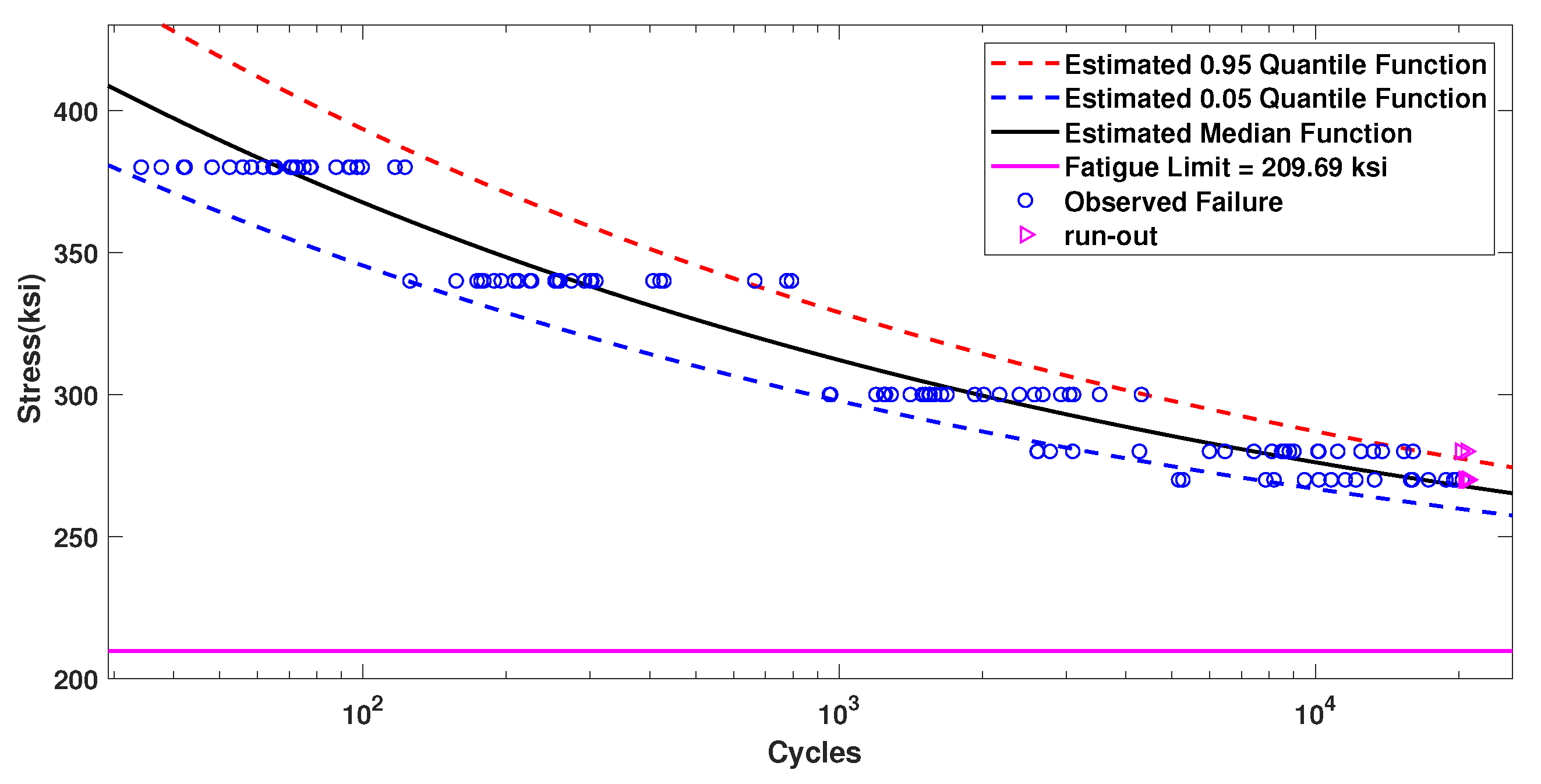
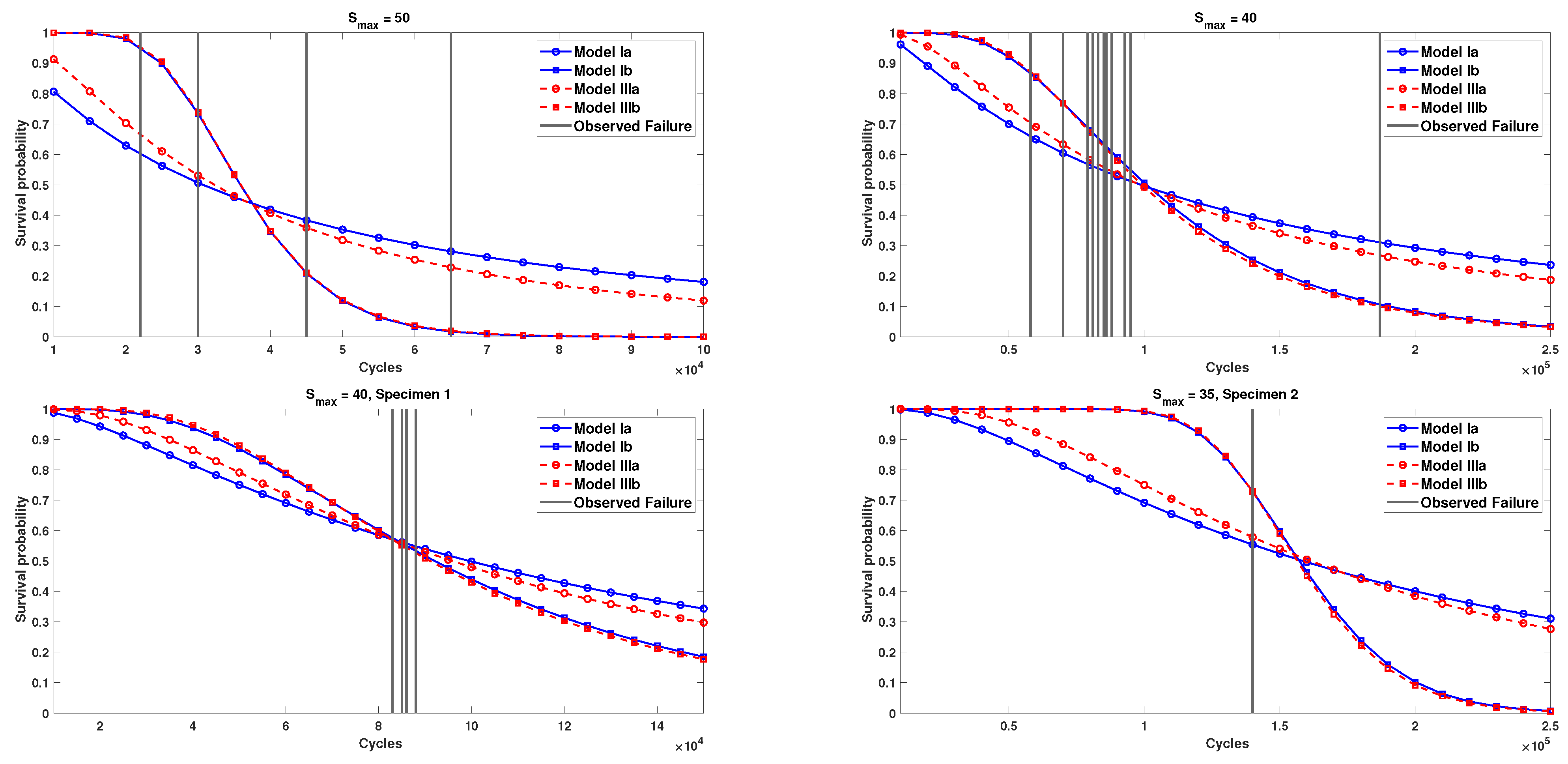
4.3. Survival Functions
5. Model Calibration and Comparison for Dataset 3
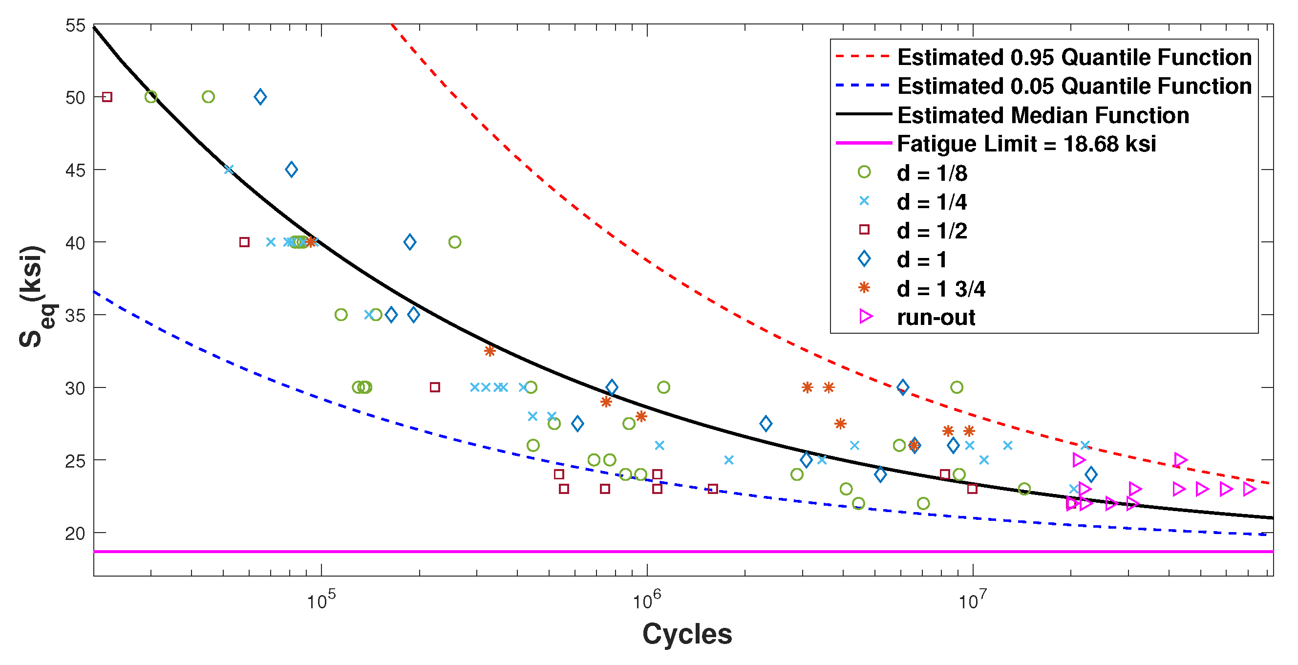
Description of Dataset 3
6. Conclusions
Author Contributions
Funding
Data Availability Statement
Acknowledgments
Conflicts of Interest
References
- Schijve, J. Fatigue of structures and materials in the 20th century and the state of the art. Int. J. Fatigue 2003, 25, 679–702. [Google Scholar] [CrossRef]
- Schijve, J. Fatigue of Structures and Materials, 2nd ed.; Springer: Berlin/Heidelberg, Germany, 2009. [Google Scholar]
- Fatemi, A.; Yang, L. Cumulative fatigue damage and life prediction theories: A survey of the state of the art for homogeneous materials. Int. J. Fatigue 1998, 20, 9–34. [Google Scholar] [CrossRef]
- Murakami, Y.; Takagi, T.; Wada, K.; Matsunaga, H. Essential structure of SN curve: Prediction of fatigue life and fatigue limit of defective materials and nature of scatter. Int. J. Fatigue 2021, 146, 106138. [Google Scholar] [CrossRef]
- Askes, H.; Susmel, L. Understanding cracked materials: Is linear elastic fracture mechanics obsolete? Fatigue Fract. Eng. Mater. Struct. 2015, 38, 154–160. [Google Scholar] [CrossRef]
- He, H.; Liu, H.; Mura, A.; Zhu, C. Gear bending fatigue life prediction based on continuum damage mechanics and linear elastic fracture mechanics. Meccanica 2023, 58, 119–135. [Google Scholar] [CrossRef]
- Yue, F.; Wu, Z. Fracture mechanical analysis of thin-walled cylindrical shells with cracks. Metals 2021, 11, 592. [Google Scholar] [CrossRef]
- Rahim, M.R.B.A.; Schmauder, S.; Manurung, Y.H.; Binkele, P.; Dusza, J.; Csanádi, T.; Ahmad, M.I.M.; Mat, M.F.; Dogahe, K.J. Assessing Fatigue Life Cycles of Material X10CrMoVNb9-1 through a Combination of Experimental and Finite Element Analysis. Metals 2023, 13, 1947. [Google Scholar] [CrossRef]
- MIL-STD-1530C; Department of Defense Standard Practice: Aircraft Structural Integrity Program (ASIP). U.S. Department of Defense: Washington, DC, USA, 2016.
- Ritchie, R.O.; Liu, D. Introduction to Fracture Mechanics; Elsevier: Amsterdam, The Netherlands, 2021. [Google Scholar]
- Berens, A.; Hovey, P.; Skinn, D. Risk Analysis for Aging Aircraft Fleets-Volume 1: Analysis, WL-TR-91-3066; Technical Report; Flight Dynamics Directorate, Wright Laboratory, Air Force Systems Command, Wright-Patterson Air Force Base: Dayton, OH, USA, 1991. [Google Scholar]
- Main, B.; Molent, L.; Singh, R.; Barter, S. Fatigue crack growth lessons from thirty-five years of the Royal Australian Air Force F/A-18 A/B hornet aircraft structural integrity program. Int. J. Fatigue 2020, 133, 105426. [Google Scholar] [CrossRef]
- White, P.; Molent, L.; Barter, S. Interpreting fatigue test results using a probabilistic fracture approach. Int. J. Fatigue 2005, 27, 752–767. [Google Scholar] [CrossRef]
- Gallagher, J.; Molent, L. The equivalence of EPS and EIFS based on the same crack growth life data. Int. J. Fatigue 2015, 80, 162–170. [Google Scholar] [CrossRef]
- Liang, Y.; Dávila, C.; Iarve, E. A reduced-input cohesive zone model with regularized extended finite element method for fatigue analysis of laminated composites in Abaqus. Compos. Struct. 2021, 275, 114494. [Google Scholar] [CrossRef]
- Babuska, I.; Sawlan, Z.; Scavino, M.; Szabó, B.; Tempone, R. Bayesian inference and model comparison for metallic fatigue data. Comput. Methods Appl. Mech. Eng. 2016, 304, 171–196. [Google Scholar] [CrossRef]
- Pascual, F.G.; Meeker, W.Q. Analysis of fatigue data with runouts based on a model with nonconstant standard deviation and a fatigue limit parameter. J. Test. Eval. 1997, 25, 292–301. [Google Scholar] [CrossRef]
- Pascual, F.G.; Meeker, W.Q. Estimating fatigue curves with the random fatigue-limit model. Technometrics 1999, 41, 277–289. [Google Scholar] [CrossRef]
- Ryan, K.J. Estimating expected information gains for experimental designs with application to the random fatigue-limit model. J. Comput. Graph. Stat. 2003, 12, 585–603. [Google Scholar] [CrossRef]
- Schijve, J. A normal distribution or a Weibull distribution for fatigue lives. Fatigue Fract. Eng. Mater. Struct. 1993, 16, 851–859. [Google Scholar] [CrossRef]
- Zou, Q.; Wen, J. Bayesian model averaging for probabilistic SN curves with probability distribution model form uncertainty. Int. J. Fatigue 2023, 177, 107955. [Google Scholar] [CrossRef]
- Birnbaum, Z.; Saunders, S. A New Family of Life Distributions. J. Appl. Probab. 1969, 6, 319–327. [Google Scholar] [CrossRef]
- Birnbaum, Z.W.; Saunders, S.C. Estimation for a family of life distributions with applications to fatigue. J. Appl. Probab. 1969, 6, 328–347. [Google Scholar] [CrossRef]
- Engelhardt, M.; Bain, L.J.; Wright, F.T. Inferences on the Parameters of the Birnbaum–Saunders Fatigue life Distribution Based on Maximum likelihood Estimation. Technometrics 1981, 23, 251–256. [Google Scholar] [CrossRef]
- Achcar, J.A. Inferences for the Birnbaum–Saunders fatigue life model using Bayesian methods. Comput. Stat. Data Anal. 1993, 15, 367–380. [Google Scholar] [CrossRef]
- Tsionas, E.G. Bayesian inference in Birnbaum–Saunders regression. Commun. Stat.-Theory Methods 2001, 30, 179–193. [Google Scholar] [CrossRef]
- Xu, A.; Tang, Y. Bayesian analysis of Birnbaum–Saunders distribution with partial information. Comput. Stat. Data Anal. 2011, 55, 2324–2333. [Google Scholar] [CrossRef]
- Rieck, J.R.; Nedelman, J.R. A log-linear model for the Birnbaum–Saunders distribution. Technometrics 1991, 33, 51–60. [Google Scholar]
- Kundu, D. Bivariate log Birnbaum–Saunders distribution. Statistics 2015, 49, 900–917. [Google Scholar] [CrossRef]
- Leiva, V. The Birnbaum–Saunders Distribution; Academic Press: Cambridge, MA, USA, 2015. [Google Scholar]
- Balakrishnan, N.; Kundu, D. Birnbaum–Saunders distribution: A review of models, analysis, and applications. Appl. Stoch. Model. Bus. Ind. 2019, 35, 4–49. [Google Scholar] [CrossRef]
- Grover, H.J.; Bishop, S.M.; Jackson, L.R. Fatigue Strengths of Aircraft Materials: Axial-Load Fatigue Tests on Unnotched Sheet Specimens of 24S-T3 and 75S-T6 Aluminum Alloys and of SAE 4130 Steel; NACA TN 2324; National Advisory Committee on Aeronautics: Washington, DC, USA, 1951. [Google Scholar]
- Hyler, W.S.; Lewis, R.A.; Grover, H.J. Experimental Investigation of Notch-Size Effects on Rotating-Beam Fatigue Behavior of 75S-T6 Aluminum Alloys; NACA TN 3291; National Advisory Committee on Aeronauticss: Washington, DC, USA, 1954. [Google Scholar]
- Shimokawa, T.; Hamaguchi, Y. Statistical evaluation of fatigue life and fatigue strength in circular-hole notched specimens of a carbon eight-harness-satin/epoxy laminate. In Statistical Research on Fatigue and Fracture (A 88-51351 22-39); Elsevier Applied Science: London, UK; New York, NY, USA, 1987; pp. 159–176. [Google Scholar]
- Akaike, H. Information Theory and An Extension of the Maximum Likelihood Principle. In Breakthroughs in Statistics, Volume I; Springer: Berlin/Heidelberg, Germany, 1992; pp. 610–624. [Google Scholar]
- Schwarz, G. Estimating the dimension of a model. Ann. Stat. 1978, 6, 461–464. [Google Scholar] [CrossRef]
- Neath, A.A.; Cavanaugh, J.E. The Bayesian information criterion: Background, derivation, and applications. Wiley Interdiscip. Rev. Comput. Stat. 2012, 4, 199–203. [Google Scholar] [CrossRef]
- Burnham, K.P.; Anderson, D.R. Model Selection and Multimodel Inference, 2nd ed.; Springer: Berlin/Heidelberg, Germany, 2002. [Google Scholar]
- Walker, K. The effect of stress ratio during crack propagation and fatigue for 2024-T3 and 7075-T6 aluminum. Eff. Environ. Complex Load Hist. Fatigue Life 1970, 462, 1–14. [Google Scholar]
- Huang, X.; Moan, T. Improved modeling of the effect of R-ratio on crack growth rate. Int. J. Fatigue 2007, 29, 591–602. [Google Scholar] [CrossRef]
- Babuška, I.; Sawlan, Z.; Scavino, M.; Szabó, B.; Tempone, R. Spatial Poisson processes for fatigue crack initiation. Comput. Methods Appl. Mech. Eng. 2019, 345, 454–475. [Google Scholar] [CrossRef]
- Chen, J.; Liu, S.; Zhang, W.; Liu, Y. Uncertainty quantification of fatigue SN curves with sparse data using hierarchical Bayesian data augmentation. Int. J. Fatigue 2020, 134, 105511. [Google Scholar] [CrossRef]
- Meeker, W.Q.; Escobar, L.A.; Pascual, F.G.; Hong, Y.; Liu, P.; Falk, W.M.; Ananthasayanam, B. Modern Statistical Models and Methods for Estimating Fatigue-Life and Fatigue-Strength Distributions from Experimental Data. arXiv 2022, arXiv:2212.04550. [Google Scholar]
- Li, Y.Z.; Zhu, S.P.; Liao, D.; Niu, X.P. Probabilistic modeling of fatigue crack growth and experimental verification. Eng. Fail. Anal. 2020, 118, 104862. [Google Scholar] [CrossRef]
- Molent, L.; Wanhill, R. Management of airframe in-service pitting corrosion by decoupling fatigue and environment. Corros. Mater. Degrad. 2021, 2, 493–511. [Google Scholar] [CrossRef]
- Zhang, Y.; Zheng, K.; Heng, J.; Zhu, J. Corrosion-fatigue evaluation of uncoated weathering steel bridges. Appl. Sci. 2019, 9, 3461. [Google Scholar] [CrossRef]


| q | Max Log-Likelihood | |||||
|---|---|---|---|---|---|---|
| Model Ia | 7.38 | −2.01 | 35.04 | 0.5628 | 0.5274 | −950.16 |
| Model IIa | 18.81 | −5.68 | 33.11 | 0.5390 | 1.54 | −960.68 |
| Model IIIa | 7.22 | −1.90 | 35.32 | 0.5574 | 0.0933 | −938.90 |
| q | Max Log-Likelihood | ||||||
|---|---|---|---|---|---|---|---|
| Model Ib | 6.72 | −1.57 | 36.21 | 0.5510 | 4.55 | −2.89 | −920.51 |
| Model IIb | 16.56 | −4.26 | 35.51 | 0.5239 | 5.54 | −3.21 | −926.97 |
| Model IIIb | 6.70 | −1.56 | 36.24 | 0.5501 | 2.90 | −2.34 | −917.38 |
| Models | Ia | Ib | IIa | IIb | IIIa | IIIb |
|---|---|---|---|---|---|---|
| Maximum log−likelihood | −950.16 | −920.51 | −960.68 | −926.97 | −938.90 | −917.38 |
| Akaike information criterion (AIC) | 1910.3 | 1853.0 | 1931.4 | 1865.9 | 1887.8 | 1846.8 |
| Bayesian information criterion (BIC) | 1922.5 | 1867.7 | 1943.6 | 1880.6 | 1900.0 | 1861.4 |
| Akaike information criterion with correction | 1911.1 | 1854.1 | 1932.1 | 1867.0 | 1888.5 | 1847.8 |
| Model | Data | q | Max Log-Likelihood | |||||
|---|---|---|---|---|---|---|---|---|
| Ia | 7.94 | −2.10 | 61.43 | 1.37 | 0.3203 | — | −403.56 | |
| IIIa | 7.89 | −2.10 | 57.643 | 1.2753 | 0.0575 | — | −399.64 | |
| Ib | 7.44 | −1.86 | 52.56 | 1.12 | 5.23 | −3.09 | −392.86 | |
| IIIb | 7.41 | −1.85 | 52.06 | 1.0986 | 3.40 | −2.50 | −392.23 | |
| Ia | 6.93 | −1.84 | 34.86 | 0.6304 | 0.5561 | — | −531.21 | |
| IIIa | 6.75 | −1.71 | 35.18 | 0.6269 | 0.0974 | — | −523.95 | |
| Ib | 6.84 | −1.75 | 36.55 | 0.5410 | 8.11 | −5.07 | −500.46 | |
| IIIb | 6.75 | −1.69 | 36.62 | 0.5388 | 6.27 | −4.41 | −499.15 |
| Model | Data | q | Max Log-Likelihood | |||||
|---|---|---|---|---|---|---|---|---|
| Ia | 7.08 | −2.11 | 23.80 | 0.3679 | 0.3203 | — | −403.56 | |
| IIIa | 7.09 | −2.10 | 23.81 | 0.2754 | 0.0575 | — | −399.64 | |
| Ib | 6.82 | −1.86 | 24.26 | 0.1156 | 4.19 | −3.09 | −392.86 | |
| IIIb | 6.80 | −1.85 | 24.31 | 0.0986 | 2.57 | −2.50 | −392.23 | |
| Ia | 6.59 | −1.84 | 22.52 | −0.3696 | 0.5561 | — | −531.21 | |
| IIIa | 6.43 | −1.71 | 22.78 | −0.3732 | 0.0974 | — | −523.95 | |
| Ib | 6.56 | −1.75 | 25.12 | −0.4590 | 7.29 | −5.07 | −500.46 | |
| IIIb | 6.54 | −1.74 | 25.19 | −0.4607 | 5.68 | −4.49 | −499.13 |
| Model | q | Max Log-Likelihood | AIC | |||||
|---|---|---|---|---|---|---|---|---|
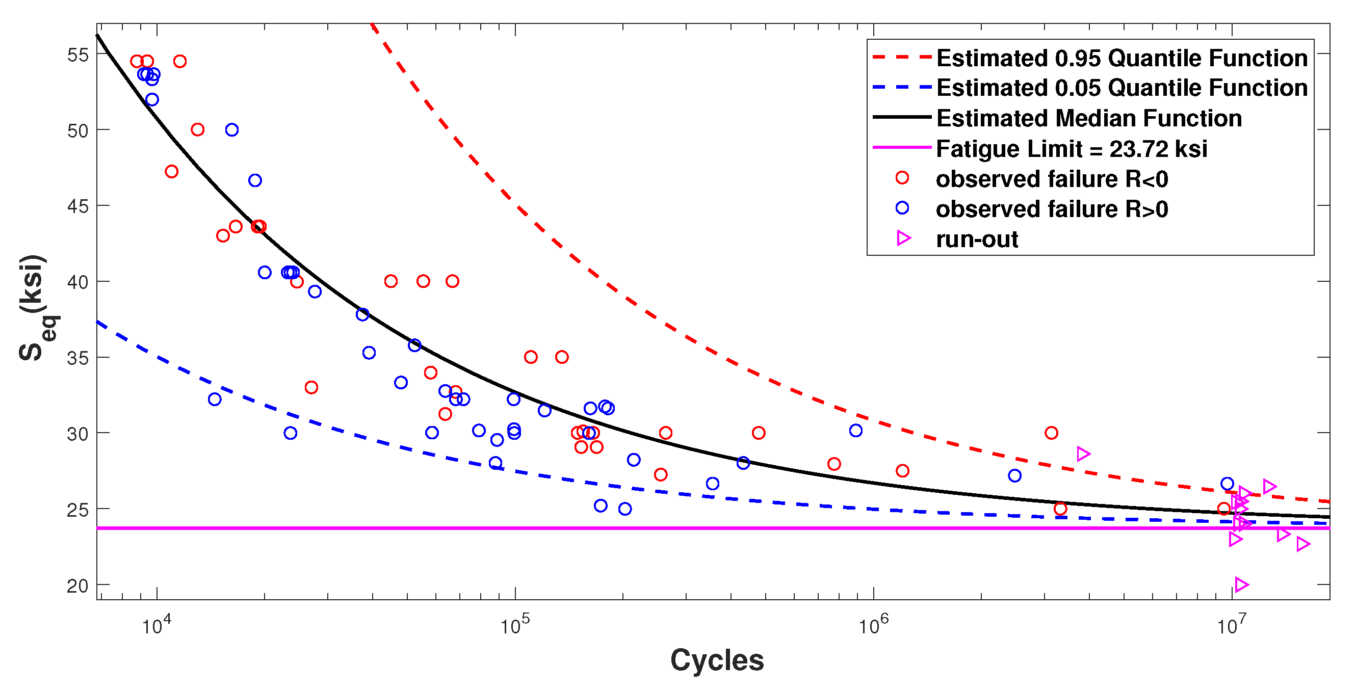
| Ia | 6.99 | −2.09 | 23.72 | 0.4310 | 0.4797 | — | −942.55 | 1895.1 |
| IIIa | 6.81 | −1.95 | 23.98 | 0.4336 | 0.0845 | — | −930.85 | 1871.7 |
| Ib | 6.58 | −1.76 | 24.56 | 0.4433 | 5.97 | −4.23 | −899.36 | 1810.7 |
| IIIb | 6.54 | −1.74 | 24.62 | 0.4436 | 4.38 | −3.65 | −897.67 | 1807.3 |
| Minimum-Section Diameter (Inches) | Number of Unnotched Specimens | Number of Run-Outs |
|---|---|---|
| 1/8 | 32 | 3 |
| 1/4 | 28 | 5 |
| 1/2 | 14 | 2 |
| 1 | 17 | 3 |
| 10 | 0 |
| Model | Specimen | Diameter | Max Log-Likelihood | |||||
|---|---|---|---|---|---|---|---|---|
| Ia | 1 | 1/8 | 7.20 | −1.73 | 21.17 | 0.4420 | — | −428.28 |
| Ib | 1 | 1/8 | 7.36 | −1.87 | 21.11 | 2.38 | −1.87 | −425.73 |
| IIIa | 1 | 1/8 | 7.17 | −1.72 | 21.23 | 0.0721 | — | −426.06 |
| IIIb | 1 | 1/8 | 7.28 | −1.82 | 21.21 | 0.88 | −1.38 | −424.62 |
| Ia | 2 | 1/4 | 8.21 | −2.69 | 21.86 | 0.4002 | — | −343.94 |
| Ib | 2 | 1/4 | 7.21 | −1.86 | 22.88 | 8.70 | −6.33 | −327.49 |
| IIIa | 2 | 1/4 | 7.96 | −2.48 | 22.16 | 0.0604 | — | −340.75 |
| IIIb | 2 | 1/4 | 7.20 | −1.85 | 22.91 | 6.86 | −5.62 | −326.85 |
| Ia | All | — | 9.03 | −3.04 | 18.68 | 0.5626 | — | −1357.8 |
| Ib | All | — | 8.23 | −2.50 | 20.49 | 3.39 | −2.53 | −1338.1 |
| IIIa | All | — | 8.73 | −2.84 | 19.24 | 0.0880 | — | −1349.6 |
| IIIb | All | — | 8.15 | −2.45 | 20.61 | 1.86 | −2.02 | −1336.1 |
| Model | |||||
|---|---|---|---|---|---|
| Ia | (7.9, 11.1) | (−4.3, −2.2) | (14.3, 21) | (0.49, 0.62) | — |
| Ib | (7.6, 9.2) | (−3.1, −2.1) | (18.5, 21.6) | (2.8, 4.6) | (−3.4, −2.1) |
| IIa | (7.8,10.3) | (−3.8, −2.2) | (15.7, 21.1) | (0.077, 0.096) | — |
| IIb | (7.6, 9.1) | (−3.1, −2.0) | (18.6, 21.7) | (1.3, 3) | (−2.9, −1.6) |
| Model | Max Log-Likelihood | |||||
|---|---|---|---|---|---|---|
| Ia | 31.56 | −5.32 | 209.69 | 0.4902 | — | −889.77 |
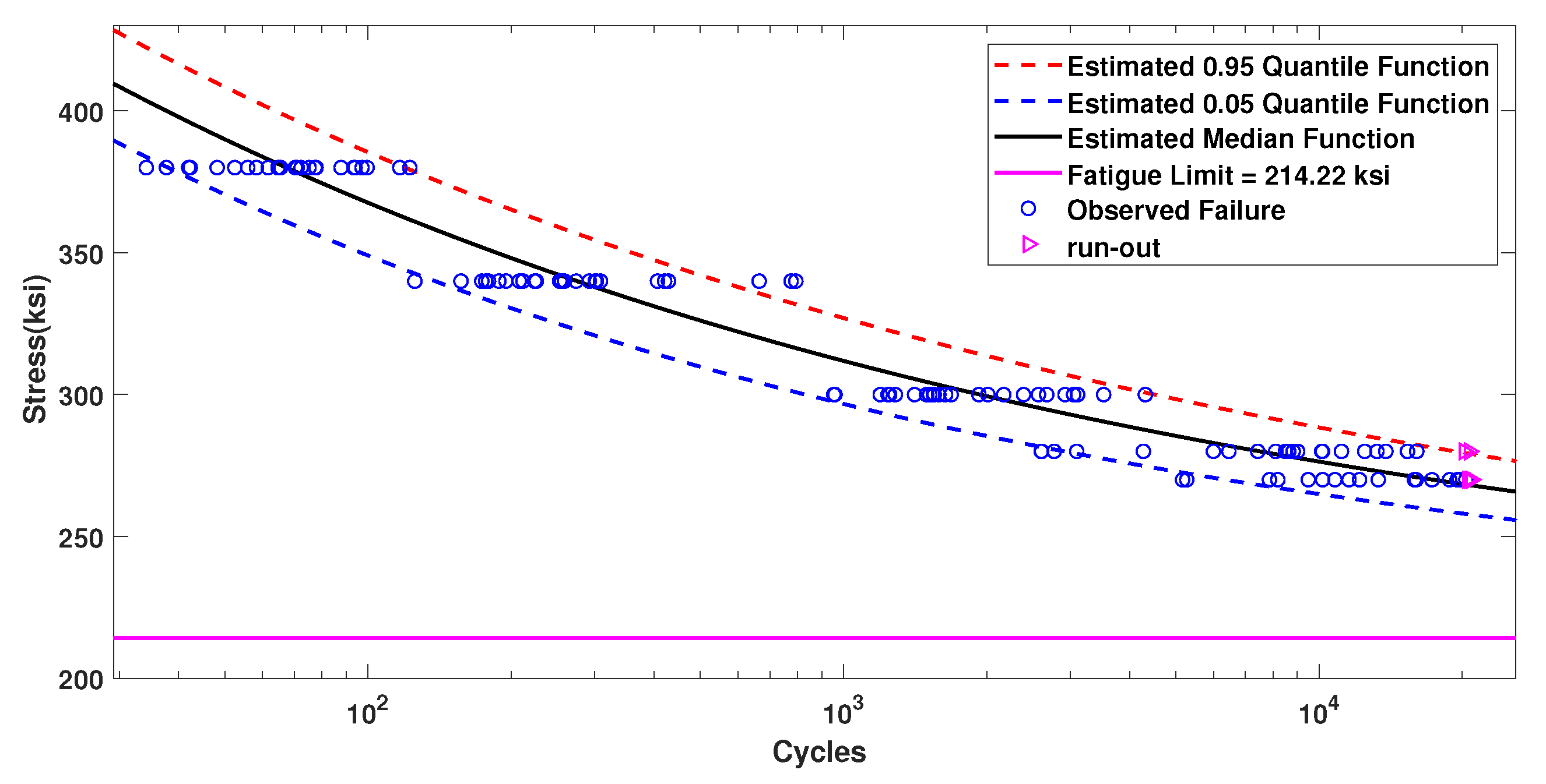
| Ib | 30.26 | −5.10 | 214.22 | 8.71 | −1.64 | −885.28 |
| IIa | 32.15 | −5.43 | 207.55 | 0.5031 | — | −889.90 |
| IIb | 30.77 | −5.18 | 212.45 | 9.01 | −1.69 | −885.17 |
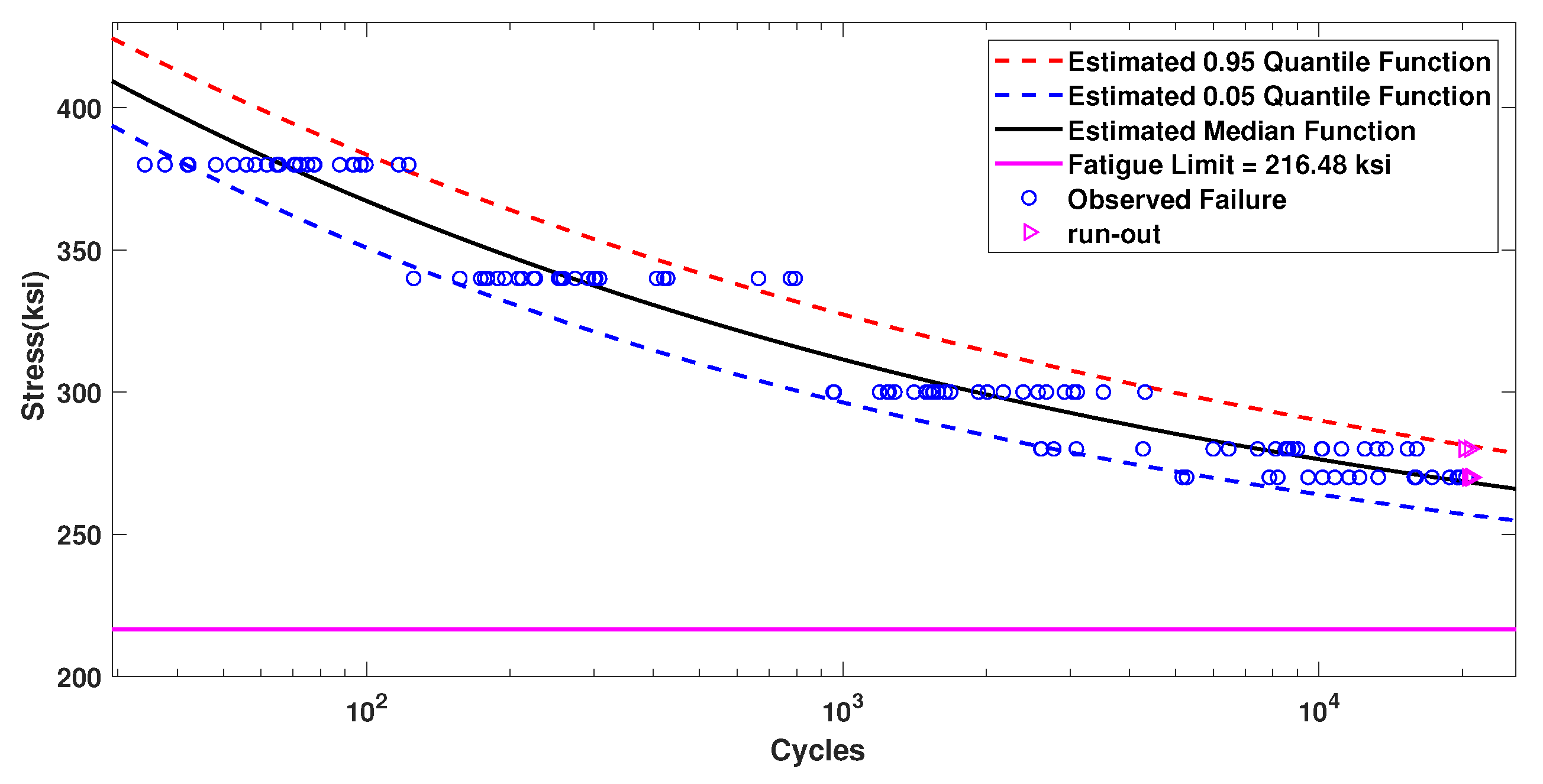
| IIIa | 29.63 | −4.99 | 216.48 | 0.0718 | — | −885.64 |
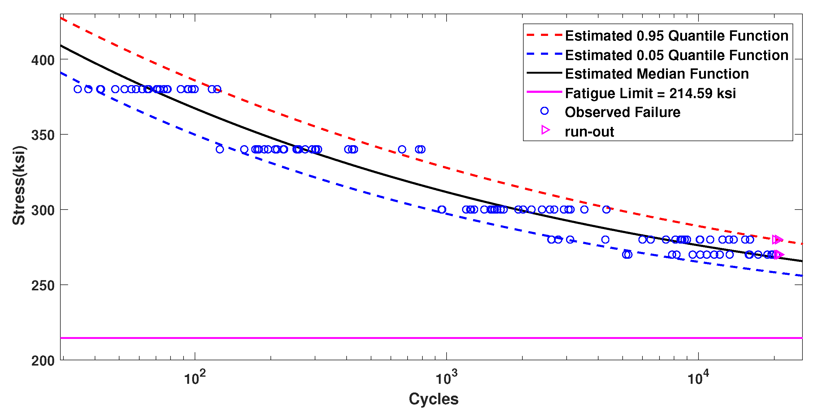
| IIIb | 30.14 | −5.08 | 214.59 | −6.84 | 0.73 | −884.67 |
| Models | Ia | Ib | IIa | IIb | IIIa | IIIb |
|---|---|---|---|---|---|---|
| Maximum log−likelihood | −889.77 | −885.28 | −889.90 | −885.17 | −885.64 | −884.67 |
| Akaike information criterion (AIC) | 1787.5 | 1780.6 | 1787.8 | 1780.3 | 1779.3 | 1779.3 |
| Bayesian information criterion (BIC) | 1798.9 | 1794.7 | 1799.1 | 1794.5 | 1790.6 | 1793.5 |
| Akaike information criterion with correction | 1787.9 | 1781.1 | 1788.1 | 1780.8 | 1779.6 | 1779.8 |
Disclaimer/Publisher’s Note: The statements, opinions and data contained in all publications are solely those of the individual author(s) and contributor(s) and not of MDPI and/or the editor(s). MDPI and/or the editor(s) disclaim responsibility for any injury to people or property resulting from any ideas, methods, instructions or products referred to in the content. |
© 2024 by the authors. Licensee MDPI, Basel, Switzerland. This article is an open access article distributed under the terms and conditions of the Creative Commons Attribution (CC BY) license (https://creativecommons.org/licenses/by/4.0/).
Share and Cite
Sawlan, Z.; Scavino, M.; Tempone, R. Modeling Metallic Fatigue Data Using the Birnbaum–Saunders Distribution. Metals 2024, 14, 508. https://doi.org/10.3390/met14050508
Sawlan Z, Scavino M, Tempone R. Modeling Metallic Fatigue Data Using the Birnbaum–Saunders Distribution. Metals. 2024; 14(5):508. https://doi.org/10.3390/met14050508
Chicago/Turabian StyleSawlan, Zaid, Marco Scavino, and Raúl Tempone. 2024. "Modeling Metallic Fatigue Data Using the Birnbaum–Saunders Distribution" Metals 14, no. 5: 508. https://doi.org/10.3390/met14050508