
Analysis of the Feeding Behavior in a Bottom-Blown Lead-Smelting Furnace
 and
and
Abstract
:1. Introduction
2. Model and Assumption
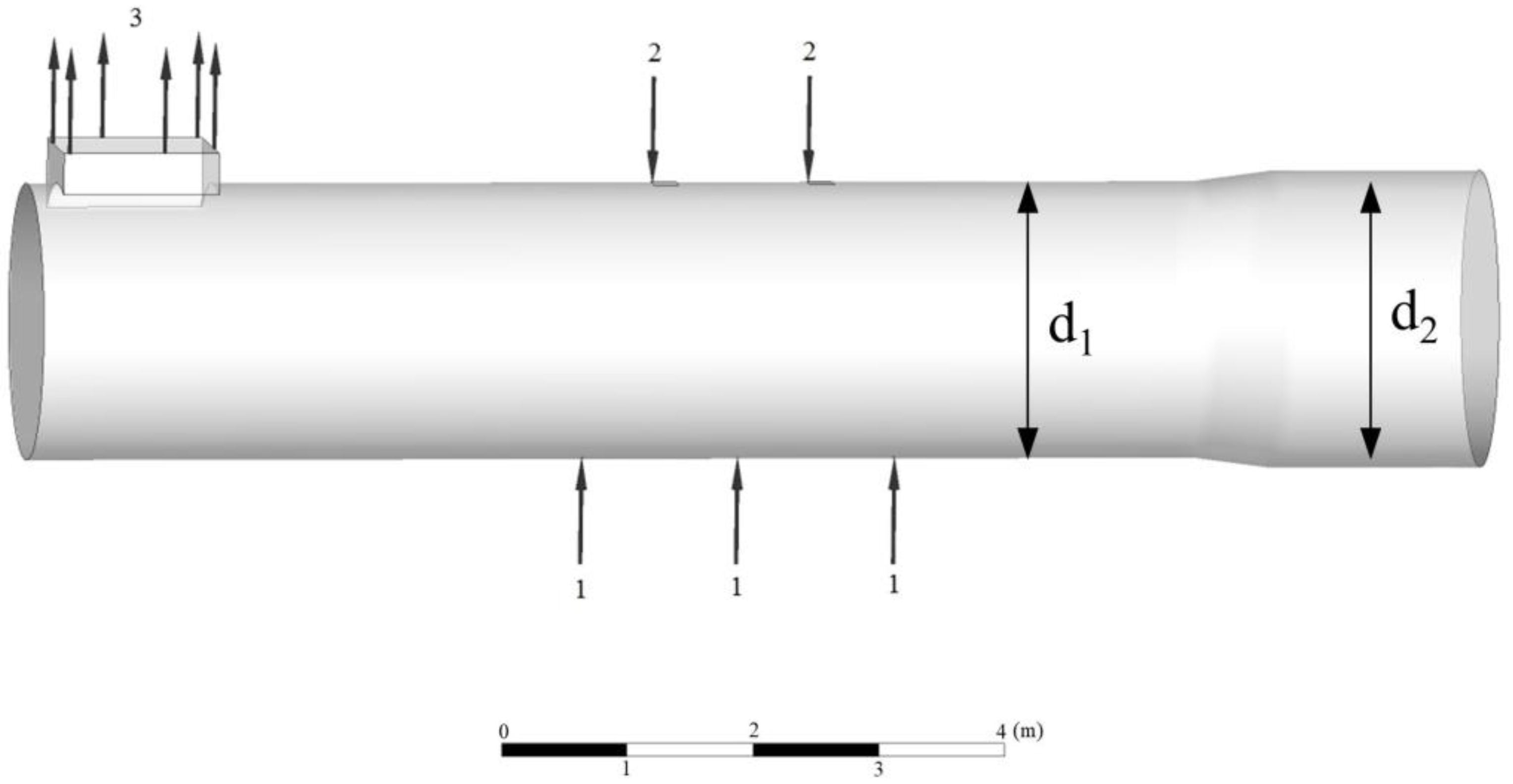
2.1. Geometric Models
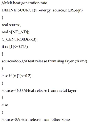
2.2. Mathematical Models
2.2.1. Continuous Phase Model
2.2.2. Turbulence Model
2.2.3. Discrete Phase Model
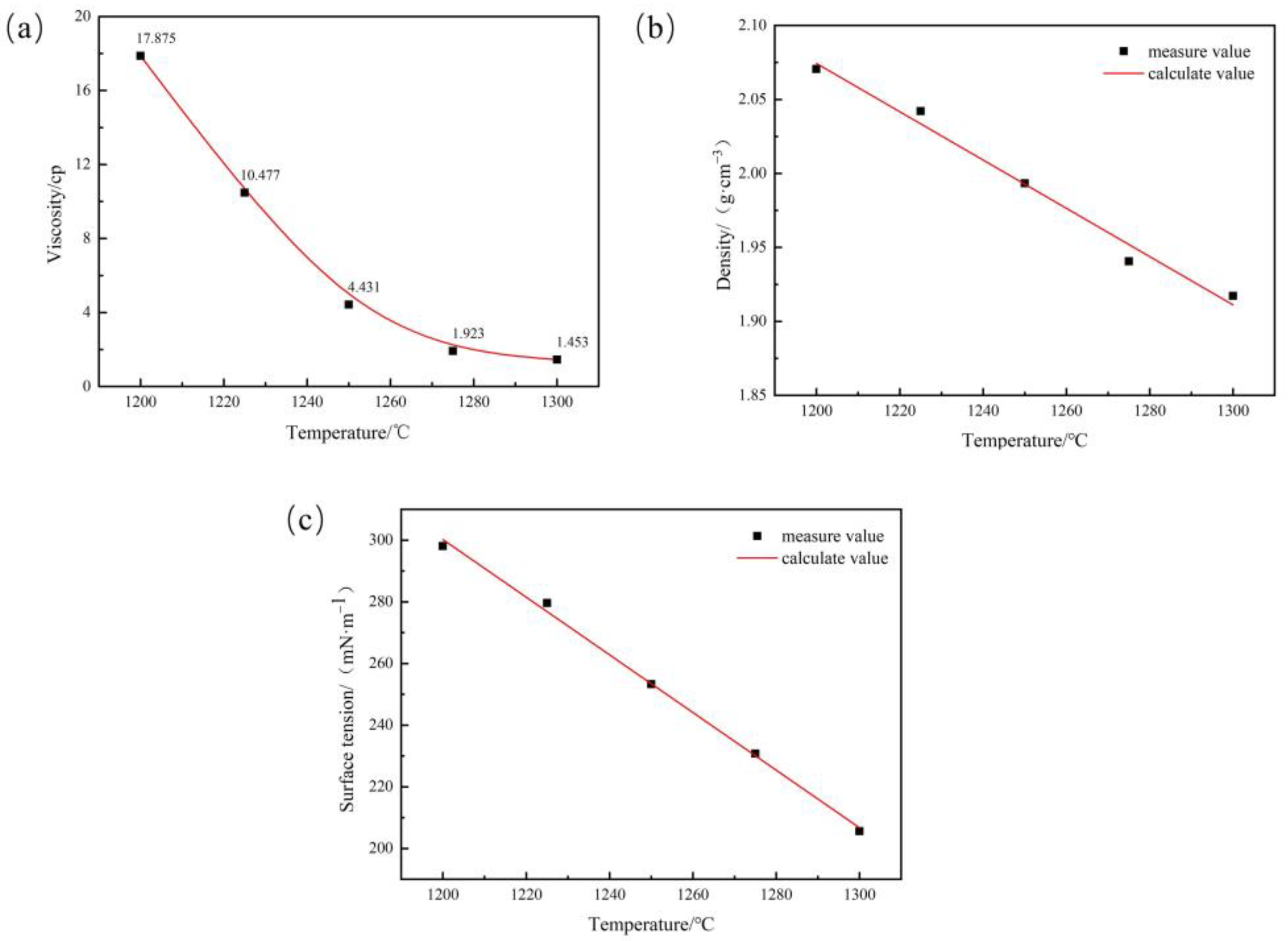
2.3. Physical Parameter Testing
2.4. Boundary Conditions and Solution Methods
3. Simulation Results
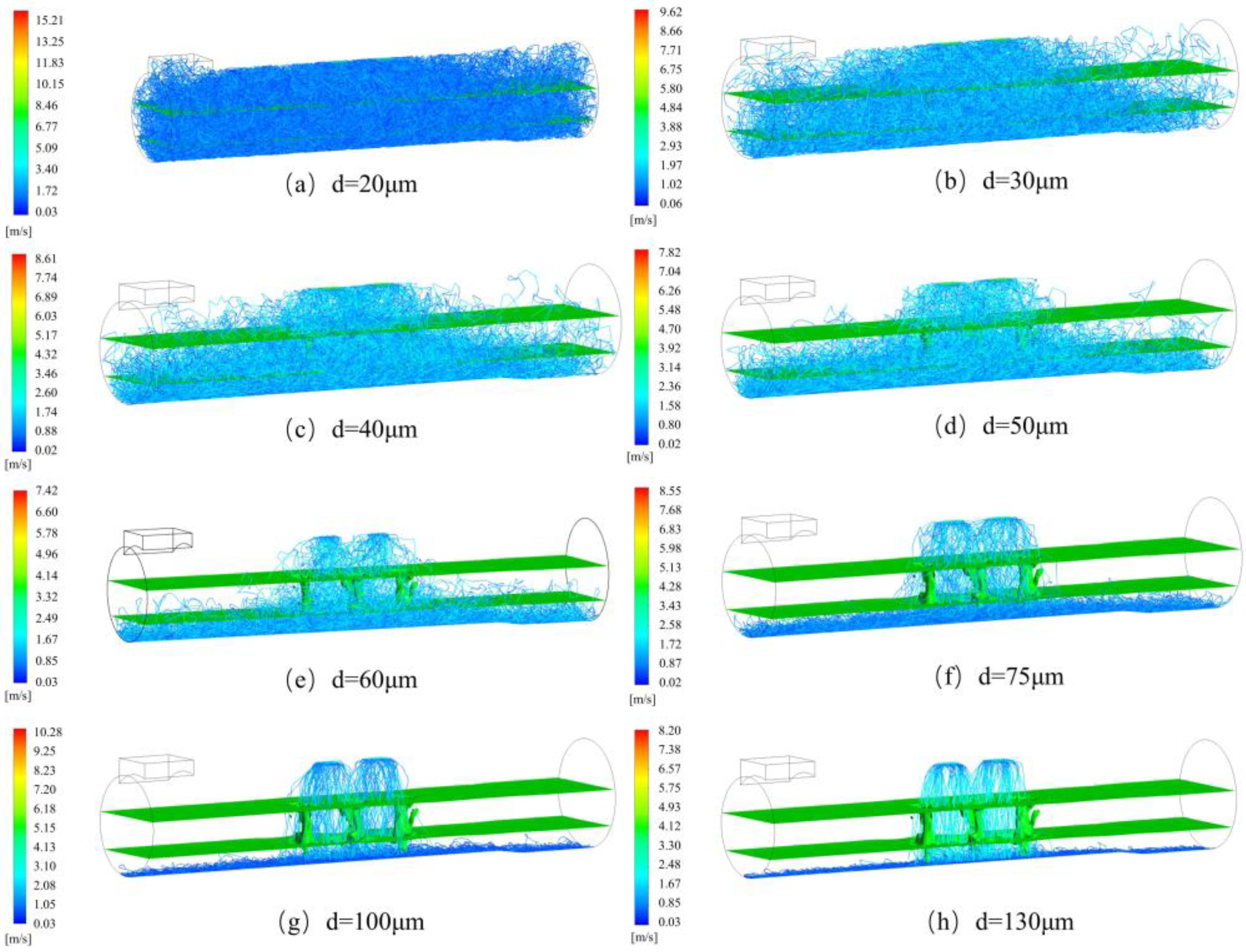
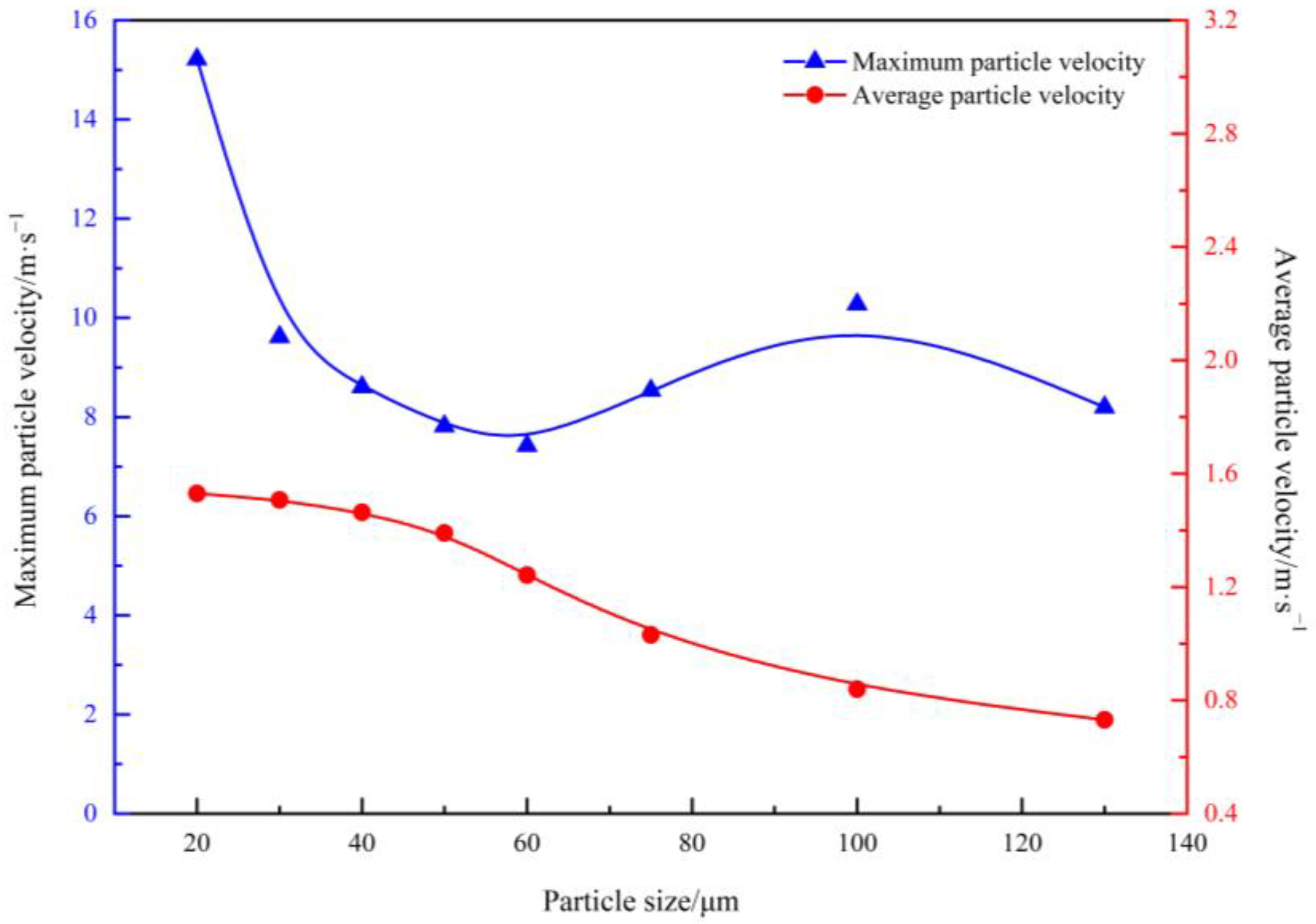
3.1. Particle Velocity Distribution
3.2. Particle Temperature Field Distribution
3.3. Particle Escape Rate and Distribution in Three Phases
4. Conclusions
- With an increase in the particle size, the average velocity of the particles decreased from 1.53 to 0.73 m/s. The maximum velocity of the particles decreased sharply in the interval of 20–40 μm, tended to level off in the interval of 40–70 μm, and decreased again in the interval of 70–130 μm. In addition, as the particle size increased, the diffusion position of the particles moved downward, from the gas layer to the metal layer.
- When the particle size was 20–50 μm, the average temperature increased with size, peaking at 970 K at 50 μm. For particles sized 50–130 μm, the average temperature decreased as the size increased, with the maximum temperature dropping from 1039 to 1020 K.
- The particle escape rate was above zero for sizes under 30 μm, with a high of 8.57% at 20 μm, causing significant material loss. Particles under 30 μm were found in the gas, slag, and matte phases, with over 20% in the gas phase. Particles over 75 μm were only in the matte phase and unevenly distributed. Particles sized 40–60 μm were in the slag and matte phases, which promoted particle reactions.
- Based on particle velocity, temperature, escape rate, and three-phase distribution, maintaining the particle size between 40–60 μm during feeding in bottom-blowing furnaces is optimal for the smelting reaction.
Author Contributions
Funding
Data Availability Statement
Conflicts of Interest
Appendix A
Appendix A1. Assumptions and Simplification
Appendix A2. Solution Method
Appendix A2.1. Boundary Conditions
Appendix A2.2. Solution Method

| Solver Type | Setting Value |
|---|---|
| Multiphase Flow Model | VOF Multiphase Flow Model |
| Turbulence Model | Standard κ-ε Turbulence Model, Standard Wall Function |
| Discrete Format | First-order Upwind Format |
| Solving Method | Standard SIMPLEC Algorithm |
| Momentum Equation | Second-order Upwind Format |
| Turbulent Kinetic Energy | First-order Upwind Format |
| Turbulent Dissipation Rate | First-order Upwind Format |
Appendix B
Appendix C
| Type | Setting Value |
|---|---|
| Multiphase flow model | Not selected |
| Energy model | Selected |
| Turbulence model | Standard turbulence model, standard wall function |
| Component equation | Finite reaction rate model |
| Discrete phase model | Selected |
| Type | Setting Value |
|---|---|
| Solver type | Based on pressure |
| Speed expression | Absolute speed |
| Gravity (m/s2) | X = 0, Y = −9.81, Z = 0 |
| Operating pressure | Atmospheric pressure |
| Type | Setting Value |
|---|---|
| Exchange source items | Selected |
| Particle calculation steps | 5000 |
| Integral scale | 5 |
| Resistance parameter | Sphere |
| Low-order format | Explicit |
| Whether to couple energy and matter | Not selected |
| Force model | Particle drag force, thermophoretic force, Stokes force, Brownian force |
| Jet type | Surface |
| Particle type | Burning |
| Particle size distribution | Unified diameter |
| Particle size (m) | 20 μm, 30 μm, 40 μm, 50 μm, 60 μm, 75 μm, 100 μm, 130 μm |
| Temperature (K) | 300 |
| Number of particles | 175 |
| Random orbit | Random discrete distribution trajectory model |
| Surface chemical reaction | customized |
Appendix D
Appendix E
Appendix F
Appendix G
| Solution Method | Set Value |
|---|---|
| Pressure–Velocity Coupling Method | SIMPLE |
| Gradient | Least Squares Element Method |
| Other Discretization | First Order Upwind Format |
| Factors | Set Value |
|---|---|
| Pressure | 0.3 |
| Density | 0.3 |
| Body Forces | 0.3 |
| Momentum | 0.3 |
| Turbulent Kinetic Energy | 0.3 |
| Turbulent Dissipation Rate | 0.3 |
| Turbulent Viscosity | 0.3 |
| Species | 0.3 |
| Energy | 0.3 |
| Discrete Phase Sources | 0.1 |
Appendix H
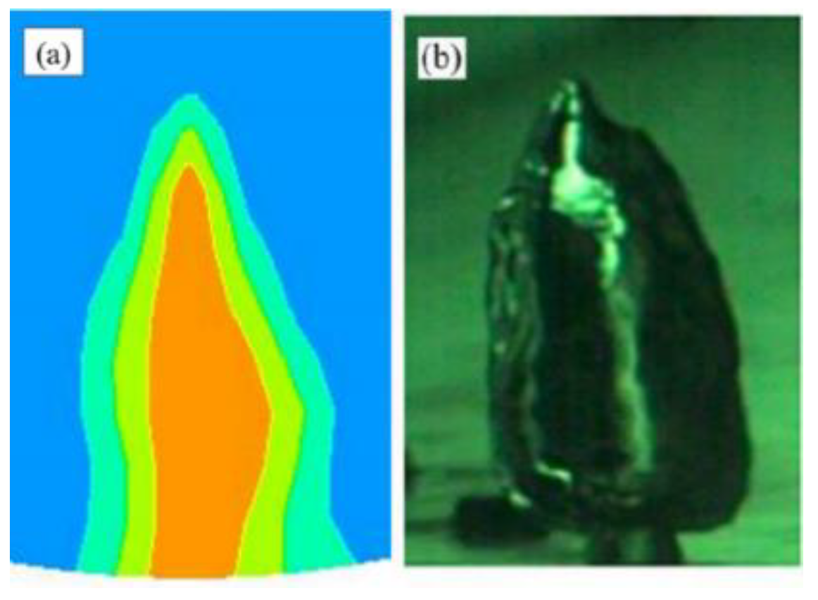
| Result | d1/d2 |
|---|---|
| Simulation | 6.5 |
| Literature | 6.7 [34] |
| Error/% | 2.99 |
References
- Sohn, H.Y.; Olivas-Martinez, M. Lead and zinc production. In Treatise on Process Metallurgy; Elsevier: Amsterdam, The Netherlands, 2024; pp. 605–624. [Google Scholar]
- Gao, G.; Wang, C.Y.; Yin, F.; Cheng, Y.X.; Yang, W.J. Situation and technology progress of lead smelting in China. Adv. Mater. Res. 2012, 581–582, 904–911. [Google Scholar] [CrossRef]
- Li, Y.G.; Jing, X.D. A decade’s production practice of JCC Kivcet technique. J. Phys. Conf. Ser. 2024, 2738, 012009. [Google Scholar]
- Li, J.D.; Zhou, P.; Liao, Z.; Chai, L.Y.; Zhou, C.Q.; Zhang, L. CFD modelling and optimization of oxygen supply mode in KIVCET smelting process. Trans. Nonferrous Met. Soc. China 2019, 29, 1560–1568. [Google Scholar] [CrossRef]
- Zhao, H.L.; Liu, F.Q.; Xiao, Y.D.; Sohn, H.Y. Computational fluid dynamics simulation of gas–matte–slag three-phase flow in an ISASMELT furnace. Metall. Mater. Trans. B 2021, 52, 3767–3776. [Google Scholar] [CrossRef]
- Zhao, H.L.; Lu, T.T.; Yin, P.; Mu, L.Z.; Liu, F.Q. An experimental and simulated study on gas-liquid flow and mixing behavior in an ISASMELT furnace. Metals 2019, 9, 565. [Google Scholar] [CrossRef]
- Rezende, J.; van Schalkwyk, R.F.; Reuter, M.A.; To Baben, M. A dynamic thermochemistry-based process model for lead smelting in the TSL process. J. Sustain. Metall. 2021, 7, 964–977. [Google Scholar] [CrossRef]
- Queneau, P.E. The QSL reactor for lead and its prospects for Ni, Cu and Fe. JOM 1989, 41, 30–35. [Google Scholar] [CrossRef]
- Song, K.Z.; Jokilaakso, A. CFD modeling of multiphase flow in an SKS furnace with new tuyere arrangements. Metall. Mater. Trans. B 2021, 53, 253–272. [Google Scholar] [CrossRef]
- Song, K.Z.; Jokilaakso, A. CFD modeling of multiphase flow in an SKS furnace: The effect of tuyere arrangements. Metall. Mater. Trans. B 2021, 52, 1772–1788. [Google Scholar] [CrossRef]
- Li, D.B.; Zhang, Z.X. The application of new lead smelting technology of oxidizing in bottom blowing furnace and reduction smelting in blast furnace. Nonferrous Met. Extr. Metall. 2003, 5, 12–13. [Google Scholar]
- Bai, L.; Xie, M.H. Pollution prevention and control measures for the bottom blowing furnace of a lead-smelting process, based on a mathematical model and simulation. J. Clean. Prod. 2017, 159, 432–445. [Google Scholar] [CrossRef]
- Jiang, B.C.; Guo, X.Y.; Wang, Q.M. Analysis of melt flow characteristics in large bottom-blowing furnace strengthened by oxygen lance jet at different positions. J. Sustain. Metall. 2023, 9, 1704–1715. [Google Scholar] [CrossRef]
- Chen, L.; Hao, Z.D.; Yang, T.Z.; Liu, W.F.; Zhang, D.C.; Zhang, L.; Bin, S.; Bin, W.D. A comparison study of the oxygen-rich side blow furnace and the oxygen-rich bottom blow furnace for liquid high lead slag reduction. JOM 2015, 67, 1123–1129. [Google Scholar] [CrossRef]
- Wang, W.; Mu, L.Z.; Zhao, H.L.; Cai, X.Y.; Liu, F.Q.; Sohn, H.Y. CFD Study on improvement of non-uniform stirring in a large bottom-blown copper smelting furnace. Min. Metall. Explor. 2024, 41, 1421–1435. [Google Scholar] [CrossRef]
- Shao, P.; Jiang, L.P. Flow and mixing behavior in a new bottom blown copper smelting furnace. Int. J. Mol. Sci. 2019, 20, 5757. [Google Scholar] [CrossRef] [PubMed]
- Wang, D.X.; Liu, Y.; Zhang, Z.M.; Zhang, T.A.; Li, X.L. PIV measurements on physical models of bottom blown oxygen copper smelting furnace. Can. Metall. Q. 2017, 56, 221–231. [Google Scholar] [CrossRef]
- Wang, W.; Cai, X.Y.; Mu, L.Z.; Lu, T.T.; Lv, C.; Zhao, H.L.; Sohn, H.Y. CFD simulation of the effects of mushroom heads in a bottom-blown copper smelting furnace. Metall. Mater. Trans. B 2023, 55, 694–708. [Google Scholar] [CrossRef]
- Cheng, D.; Xu, H.; Zhao, L.; Dong, H.; Zhang, Z. Effect of swirling gas inlet design on particle motion and decomposition in magnesite flash calciner. Chem. Eng. Res. Des. 2024, 206, 386–396. [Google Scholar] [CrossRef]
- Schmidt, A.; Montenegro, V.; Reuter, M.; Charitos, A.; Stelter, M.; Richter, A. CFD study on the physical behavior of flue dust in an industrial-scale copper waste heat boiler. Metall. Mater. Trans. B 2022, 53, 537–547. [Google Scholar] [CrossRef]
- Rajabi, N.; Ghodrat, M.; Moghiman, M. Numerical simulation of the effect of sulfide concentrate particle size on pollutant emission from flash smelting furnace. Int. J. Environ. Sci. Technol. 2021, 18, 2925–2936. [Google Scholar] [CrossRef]
- Duraisamy, K.; Iaccarino, G.; Xiao, H. Turbulence modeling in the age of data. Annu. Rev. Fluid Mech. 2019, 51, 357–377. [Google Scholar] [CrossRef]
- Patel, V.C.; Rodi, W.; Scheuerer, G. Turbulence models for near-wall and low Reynolds number flows-a review. AIAA J. 1985, 23, 1308–1319. [Google Scholar] [CrossRef]
- Nagano, Y.; Hishida, M. Improved form of the κ-ε model for wall turbulent shear flows. ASME J. Fluids Eng. 1987, 109, 156–160. [Google Scholar] [CrossRef]
- OuYang, K.; Dou, Z.; Zhang, T.; Liu, Y. Effect of ZnO/PbO and Fe/SiO2 ratio on viscosity of lead smelting slags. J. Min. Metall. Sect. B Metall. 2020, 56, 27–33. [Google Scholar] [CrossRef]
- Jensen, B.B.B. Numerical study of influence of inlet turbulence parameters on turbulence intensity in the flow domain: Incompressible flow in pipe system. Proc. Inst. Mech. Eng. Part E J. Process Mech. Eng. 2007, 221, 177–186. [Google Scholar] [CrossRef]
- Zamora, B.; Kaiser, A.S.; Viedma, A. On the effects of Rayleigh number and inlet turbulence intensity upon the buoyancy-induced mass flow rate in sloping and convergent channels. Int. J. Heat Mass Transf. 2008, 51, 4985–5000. [Google Scholar] [CrossRef]
- Minkowycz, W.J.; Abraham, J.P.; Sparrow, E.M. Numerical simulation of laminar breakdown and subsequent intermittent and turbulent flow in parallel-plate channels: Effects of inlet velocity profile and turbulence intensity. Int. J. Heat Mass Transf. 2009, 52, 4040–4046. [Google Scholar] [CrossRef]
- Chattopadhyay, H.; Murmu, S.C. Effect of inlet turbulence intensity on transport phenomena over bluff bodies. Int. J. Fluid Mech. Res. 2020, 47, 485–499. [Google Scholar] [CrossRef]
- Su, Y.; Davidson, J.H.; Kulacki, F.A. Numerical study on mixed convection from a constant wall temperature circular cylinder in zero-mean velocity oscillating cooling flows. Int. J. Heat Fluid Flow 2013, 44, 95–107. [Google Scholar] [CrossRef]
- Son, J.S.; Hanratty, T.J. Velocity gradients at the wall for flow around a cylinder at Reynolds numbers from 5 × 10³ to 105. J. Fluid Mech. 1969, 35, 353–368. [Google Scholar] [CrossRef]
- Kaya, F.; Karagoz, I.J.C.E. Performance analysis of numerical schemes in highly swirling turbulent flows in cyclones. Curr. Sci. 2008, 94, 1273–1278. [Google Scholar]
- Bal, M.; Kayansalçik, G.; Ertunç, Ö.; Böke, Y.E. Benchmark study of 2D and 3D VOF simulations of a simplex nozzle using a hybrid RANS-LES approach. Fuel 2022, 319, 123695. [Google Scholar] [CrossRef]
- Yan, H.J.; Xia, T.; Liu, L.; He, Q.A.; He, Z.J.; Li, Q.Q. Numerical simulation and structural optimization of gas-liquid two-phase flow in reduction furnace of lead-rich slag. Chin. J. Nonferrous Met. 2014, 24, 2642–2651. [Google Scholar]
- Yan, H.J.; Liu, F.K.; Zhang, Z.Y.; Gao, Q.; Liu, L.; Cui, Z.X.; Shen, D.B. Influence of lance arrangement on bottom-blowing bath smelting process. Chin. J. Nonferrous Met. 2012, 22, 2393–2400. [Google Scholar]
- Jiang, B.C.; Guo, X.Y.; Wang, Q.M. Two-dimensional analysis of melt pneumatic stirring in large bottom-blowing furnace based on CFD. Nonferrous Met. 2023, 6, 39–50. (In Chinese) [Google Scholar]
- Hu, H.; Yang, L.; Guo, Y.; Chen, F.; Wang, S.; Zheng, F.; Li, B. Numerical simulation of bottom-blowing stirring in different smelting stages of electric arc furnace steelmaking. Metals 2021, 11, 799. [Google Scholar] [CrossRef]


| Author | Focus Area | Ref. |
|---|---|---|
| Wang et al. | Used the VOF model to simulate the fluid flow in a copper bottom-blown smelting furnace, and improved the stirring effect in the molten bath by optimizing the oxygen injector arrangement and blowing parameters | [15] |
| Shao et al. | Developed a mathematical model to describe gas–liquid flow and mixing behavior in a bottom-blown oxygen–copper smelting furnace, and the model validation was carried out through a water model experiment | [16] |
| Wang et al. | Established a 1/5 scaled physical slice model of a bottom-blown oxygen–copper smelting furnace to investigate the flow field characteristics in the pool and in the freeboard above the pool | [17] |
| Wang et al. | Used The VOF multiphase flow model coupled with the standard κ-ε turbulence model to study the effects of the effect of radially and axially inclined mushroom heads on the flow distribution and the splash rate a bottom-blown copper smelting furnace | [18] |
| Cheng et al. | Used the discrete phase model (DPM) to analyze the effect of swirling gas inlet design on particle motion and decomposition in magnesia flash calciner (MFC) | [19] |
| Schmidt et al. | Predicted the size-dependent particle sedimentation and the risk areas for flue dust accretions by establishing a three-dimensional CFD model | [20] |
| Rajabi et al. | Studied the effects of sulfide concentrate particle size on pollutant emissions from a flash smelting furnace through numerical simulation | [21] |
| Equation | |||
|---|---|---|---|
| Continuity equation | 1 | 0 | 0 |
| Momentum equation | v | ||
| Energy equation | h | ||
| Species transport equation | Y1 |
| Type | Numerical Value |
|---|---|
| Metal density/g·cm−3 | 11.3406 |
| Metal viscosity/cP | 189.1 |
| Slag density/g·cm−3 | 1.9934 |
| Slag viscosity/cP | 1464 |
| Gas density/g·cm−3 | 1.02 × 10⁻³ |
| Gas viscosity/cP | 5.35 × 10⁻² |
| Particle Size/μm | Number Tracked | Escaped | Remained | Gas Phase | Slag Phase | Metal Phase | Particle Escape Rate/% |
|---|---|---|---|---|---|---|---|
| 20 | 175 | 15 | 160 | 42 | 84 | 35 | 8.57 |
| 30 | 175 | 2 | 173 | 35 | 82 | 56 | 1.14 |
| 40 | 175 | 0 | 175 | 0 | 91 | 84 | 0 |
| 50 | 175 | 0 | 175 | 0 | 70 | 105 | 0 |
| 60 | 175 | 0 | 175 | 0 | 56 | 119 | 0 |
| 75 | 175 | 0 | 175 | 0 | 0 | 175 | 0 |
| 100 | 175 | 0 | 175 | 0 | 0 | 175 | 0 |
| 130 | 175 | 0 | 175 | 0 | 0 | 175 | 0 |
Disclaimer/Publisher’s Note: The statements, opinions and data contained in all publications are solely those of the individual author(s) and contributor(s) and not of MDPI and/or the editor(s). MDPI and/or the editor(s) disclaim responsibility for any injury to people or property resulting from any ideas, methods, instructions or products referred to in the content. |
© 2024 by the authors. Licensee MDPI, Basel, Switzerland. This article is an open access article distributed under the terms and conditions of the Creative Commons Attribution (CC BY) license (https://creativecommons.org/licenses/by/4.0/).
Share and Cite
Sun, K.; Jie, X.; Zhang, Y.; Gao, W.; Northwood, D.O.; Waters, K.E.; Ma, H. Analysis of the Feeding Behavior in a Bottom-Blown Lead-Smelting Furnace. Metals 2024, 14, 906. https://doi.org/10.3390/met14080906
Sun K, Jie X, Zhang Y, Gao W, Northwood DO, Waters KE, Ma H. Analysis of the Feeding Behavior in a Bottom-Blown Lead-Smelting Furnace. Metals. 2024; 14(8):906. https://doi.org/10.3390/met14080906
Chicago/Turabian StyleSun, Kena, Xiaowu Jie, Yonglu Zhang, Wei Gao, Derek O. Northwood, Kristian E. Waters, and Hao Ma. 2024. "Analysis of the Feeding Behavior in a Bottom-Blown Lead-Smelting Furnace" Metals 14, no. 8: 906. https://doi.org/10.3390/met14080906