Modeling the Impact of Grain Size on Corrosion Behavior of Ni-Based Alloys in Molten Chloride Salt via Cellular Automata

Abstract

Molten chloride salts hold significant promise as both thermal transfer and storage media for next-generation concentrated solar power (CSP) systems. However, molten chlorides pose a considerable corrosion risk to structural materials, particularly Ni-based alloys. One approach to enhancing corrosion resistance is through the optimization of grain structure; however, it remains uncertain whether increasing or decreasing grain size enhances corrosion resistance. A cellular automata (CA) program was developed to evaluate the interplay between grain size and corrosion in Ni-based alloy. Our CA program tracks alloy composition, surface roughness, and thickness loss via a graphical user interface, displaying corrosion and diffusion status, and multiple user input cards for tuning the simulation. CA simulations of Inconel 625 indicate enhanced corrosion resistance with increased grain size, with passivating oxides offering limited protection. Additionally, the temporal evolution of alloy surface roughness demonstrates notable fluctuations, with abrupt increases attributed to corrosion along vertical grain boundaries and sudden decreases to grain detachment from the protective film.

1. Introduction

Concentrated solar power (CSP) has emerged as one of the most important renewable energy sources [1]. Benefiting from good thermal properties and low cost [2], molten chloride salts are a promising option for heat transfer and thermal storage media for next-generation CSP systems. But hot chloride salts are very corrosive to many components, such as piping, storage tanks, and heat exchangers. Ni-based alloys, such as Inconel 625, have shown excellent mechanical properties and good corrosion resistance, making them promising candidates for structural materials in CSP systems.

While promising, these alloys are still not corrosion-resistant enough to withstand long durations in high-temperature chloride salts. Research has shown that corrosion rates of Ni-based alloys in molten chloride salts typically exceed 100 $\mathsf{\mu }$m/year [3], much larger than the CSP target of 20 $\mathsf{\mu }$m/year. In the last decade, there have been multiple experimental studies on corrosion behaviors of Ni-based alloys in molten chloride salts attempting to improve corrosion resistance. For instance, Pragnya et al. evaluated the influence of H${ }_2$O and O${ }_2$ incorporated in the salt NaCl-KCl-MgCl${ }_2$ on the corrosion behavior of Inconel 625 at 700 ${ }^{°}$C [3]. The authors observed a five-fold increase in corrosion rate when the salts were exposed to air. Sun et al. explored the corrosion behavior of different Ni-based alloys in the salt NaCl-KCl-MgCl${ }_2$ at 700 ${ }^{°}$C and found that Ni-Mo-Cr alloys display better corrosion resistance than Ni-Fe-Cr alloys [4]. Corrosion resistance of Inconel 625, Hastelloy X, and Hastelloy B-3 in NaCl-CaCl${ }_2$-MgCl${ }_2$ with air at 600 ${ }^{°}$C was compared by Liu et al., reporting the corrosion resistance of the three alloys as Inconel 625 > Hastelloy X > Hastelloy B-3 [5]. Ravi Shankar et al. evaluated the corrosion resistance of steels (2.25 Cr-1 Mo, 9 Cr-1 Mo) and Ni-based alloys (600, 625, 690) in LiCl-KCl molten salt at 600 ${ }^{°}$C; the mass loss indicates that Ni-alloys are more corrosion-resistant than either steel composition [6]. Tests by Cho et al. on Haynes 263, Inconel 600, and Inconel 625 corroded in LiCl-Li${ }_2$O between 650 and 850 ${ }^{°}$C indicated that Haynes 263 was the least susceptible, attributing the performance to a more dense and continuous oxide layer, while Inconel 625 suffers both uniform and intergranular corrosion and with the worst performance [7]. Corrosion rates of Hastelloy C-276, Inconel 600, and Inconel 625 in molten salt LiF-BeF${ }_2$ at 600 ${ }^{°}$C were reported by Kondo et al. as 3.4 $\mathsf{\mu }$m/year, 2.8 $\mathsf{\mu }$m/year, and 1.1 $\mathsf{\mu }$m/year, respectively; Cr depletion was identified as the key driver of corrosion [8].

These studies focused on improving corrosion resistance by alloy material selection or purifying the corrosion environment. To date, there has been relatively little research on the grain size effect of Ni-based alloy on its corrosion resistance to molten chloride salts. Effects of grain size on corrosion performance have been inconsistent, due to the unknown balance between protective surface oxides and number of corrosion initiation sites [9]. A reduction in grain size leads to increased grain boundary density and may improve the corrosion resistance by facilitating surface-protective oxide formation; however, fine-grained surface structure provides more initiation sites for localized intergranular corrosion, which may result in corrosion acceleration [9].

To assess the grain size effects, we developed a cellular automata (CA) program to simulate corrosion of Ni-based alloys in molten chloride salt. The CA program provides insights into the dynamic processes of chemical reaction and diffusion, enhancing our understanding of how grain size affects the corrosion behavior. Moreover, our CA program allows the user to finely tune a variety of parameters, such as grain size, grain boundary width, material composition, chemical reaction types and rates, diffusion coefficient, etc. In this paper, we present the design and development of the CA program as well as the simulation results obtained.

2. Materials and Methods

A cellular automaton (CA), based on a discretized description of time and space, is used to model complex homogeneous and heterogeneous dynamical systems. It has wide applications in physical systems, chemical reactions, biological processes, multiphase flows, etc. [10,11]. Diffusion (mass transfer) and chemical reactions are the dominant drivers in corrosion and have been extensively studied using CA models [12,13,14,15,16,17,18,19]. Fundamentally, a CA model space divides the geometry into a regular lattice of cells, with each cell assigned a particular state. Diffusion and chemical reaction rules used in simulating the time-dependent evolution of cell states are derived from Chopard and Droz [20].

Corrosion reactions of Ni-based alloys in molten salt can be simplified as follows. The background O${ }_2$ and H${ }_2$O react with salt, producing Cl${ }_2$, which is very corrosive to common alloy elements, such as Cr. Chromium is easily oxidized by Cl${ }_2$; the resultant CrCl${ }_4$ then diffuses back into the salt. Equations (1)–(3) below depict the reaction of MgCl${ }_2$ with Cr in Ni-based alloy.

$${\mathrm{MgCl}}_2+{\mathrm{H}}_2\mathrm{O}\to \mathrm{MgO}+2\mathrm{HCl}$$

(1)

$$4\mathrm{HCl}+{\mathrm{O}}_2\to 2{\mathrm{Cl}}_2+{\mathrm{H}}_2\mathrm{O}$$

(2)

$$\mathrm{Cr}+2{\mathrm{Cl}}_2\to {\mathrm{CrCl}}_4$$

(3)

To mimic the process described above, each cell in the CA model is associated with three states: (i) material name, (ii) number of Cl${ }_2$, and (iii) number of O${ }_2$. Figure 1A depicts state (i), the defined material, in which each cell is assigned elements based on material composition. For instance, Inconel 625 mainly contains Ni, Cr, and Mo, represented by yellow, green, and blue, respectively. State (ii) is depicted in Figure 1B, in which the colors represent the number of Cl${ }_2$ in the cell (1–4), in which the top layer is the molten salt where the corrosive Cl${ }_2$ is formed, and as such, it is set to 4 (red, maximum count) at the beginning of each generation. The number is gradually decreased to 0, which is the bottom sink layer. Similarly, state (iii), for the number of O${ }_2$, is illustrated in Figure 1C, in which the five different colors (brown, orange, light blue, blue, and dark blue) represent 0 to 4, respectively.

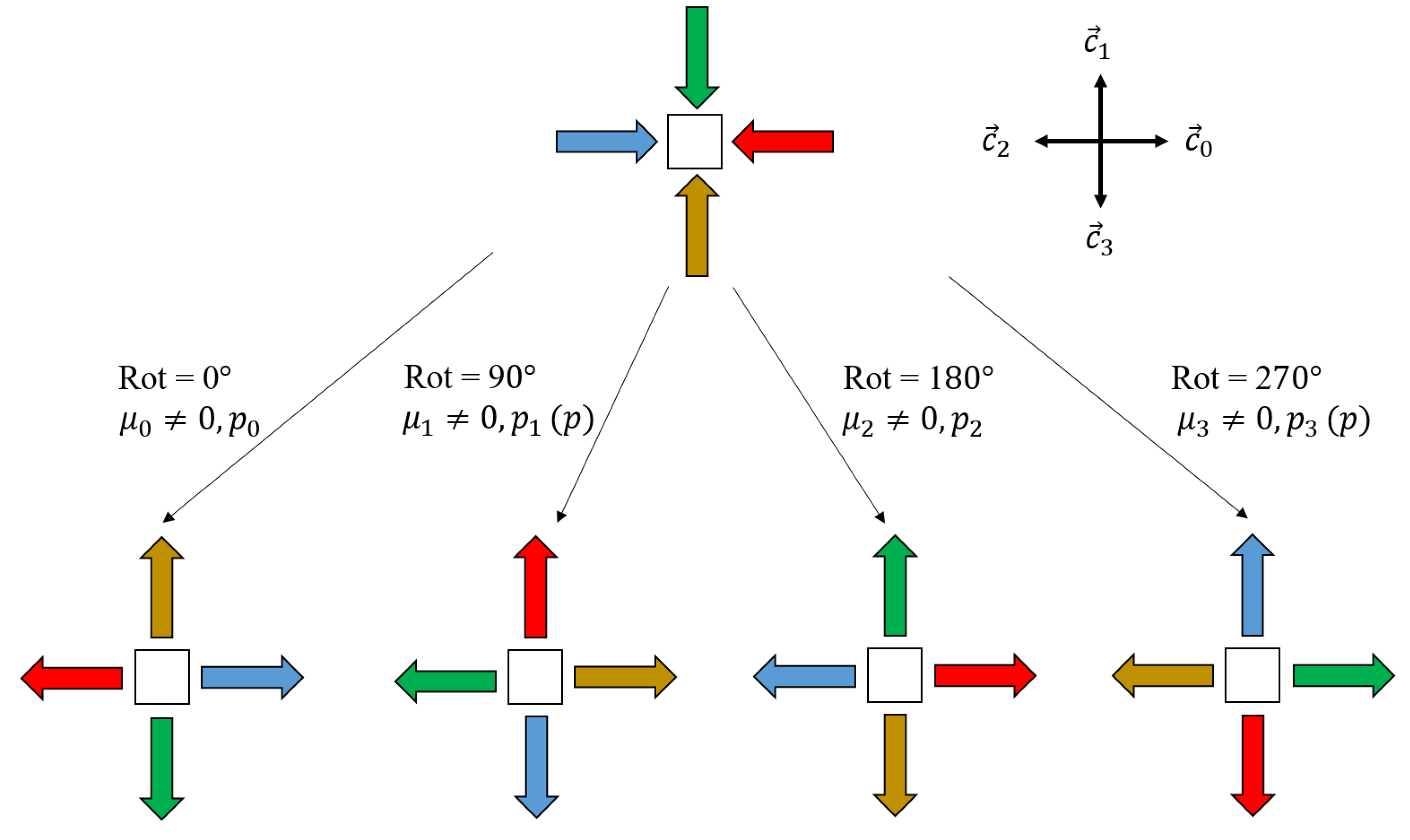
2.1. Diffusion Model

Diffusion obeys the mass conservation law, as shown in Equation (4).

$${\partial }_t\rho +\nabla ·\overrightarrow{J}=0$$

(4)

where $\rho$ is the particle density and $\overrightarrow{J}$ is the particle current, which can be expressed in terms of the diffusion constant D and $\rho$:

$$\overrightarrow{J}=-D\nabla \rho$$

(5)

Combining Equations (4) and (5) yields Fick’s law, Equation (6), which describes the diffusion from the macroscopic view.

$${\partial }_t\rho =D{\nabla }^2\rho$$

(6)

Microscopically, diffusion dynamics can be treated as the random walks of many particles, with only the total number of particles being conserved. Allowing for complete randomness may cause an infinite number of particles to occupy the same cell, violating the exclusion principle of cellular automata. The exclusion principle prohibits two cells from simultaneously occupying the same space or state within the same neighborhood or grid. To resolve this issue, a direction is assigned to each particle and there is at most one particle per direction per cell, resulting in a total number of possible directions, d.

In this work, a two-dimensional square lattice is applied in the CA simulation. We use the von Neumann neighborhood, as displayed in Figure 2, to constrain the directions of diffusing species. The red cell represents the central cell to be updated based on the states of four black neighbors: north, east, south, and west. Thus, there are at most four same particles existing in one cell.

The random walk can be acquired by permuting the directions of all entering particles. Under the exclusion principle, there are $4!=24$ ways to shuffle the directions; however, it is sufficient to use four of them to generate a random walk. Figure 3 shows a cyclic permutation, with each permutation rotated clockwise by ${90}^{°}·i(i\in 0,1,2,3)$, each with a probability of $p_i$. A boolean variable, ${\mathsf{\mu }}_i$, is constrained by Equation (7), which implies that there is exactly one ${\mathsf{\mu }}_i=1$. In the top right corner of Figure 3, ${\overrightarrow{c}}_i$ denotes lattice direction.

$$\sum _{l=0}^3{\mathsf{\mu }}_l=1$$

(7)

Let $n_i(\overrightarrow{r},t)$ represent the number of particles entering site $\overrightarrow{r}$ from direction ${\overrightarrow{c}}_i$ at time t. The random motion can be expressed by Equation (8).

$$n_i(\overrightarrow{r}+\lambda {\overrightarrow{c}}_i,t+\tau )=\sum _{l=0}^3{\mathsf{\mu }}_l{n}_{i+l}(\overrightarrow{r},t)$$

(8)

The value of ${\mathsf{\mu }}_i$ is determined by probabilities given. Symmetry leads to the constraint:

$$p_1=p_3=p$$

(9)

In addition, the probabilities sum to 1, that is,

$$p_0+2p+p2=1$$

(10)

Macroscopic diffusion behavior of Fick’s law (Equation (6)) can be linked to the microscopic random motion probabilities, $p_1$, by applying a Taylor series expansion to Equation (8), yielding Equation (11), in which $\lambda$ and $\tau$ represent the lattice spacing and time step, respectively. The diffusion coefficient, D, can be adjusted via changing probabilities. For instance, when $p_2$ is close to 1, Equation (10) indicates that p is close to 0, and therefore, D is very small; conversely, when $p_0$ is close to 1, D becomes very large.

$$D={\displaystyle \frac{{\lambda }^2}{\tau }}\left[{\displaystyle \frac{1}{4(p+p_2)}}-{\displaystyle \frac{1}{4}}\right]={\displaystyle \frac{{\lambda }^2}{\tau }}\left[{\displaystyle \frac{p+p_0}{4(1-p-p_0)}}\right]$$

(11)

In our CA diffusion program, the number of particles and their original directions for each cell are derived from the previous generation. Subsequent directions of those particles in the current generation are shuffled based on their original direction and the predefined values of $p_0$ and $p_2$ (p can be derived by Equation (10)), representing the diffusion coefficient of this cell. A stationary source–sink model is used to simulate one plate (source) on the top of the board to continuously inject particles to the system, and another plate (sink) at the bottom of the board to absorb all particles reaching it.

2.2. Corrosion Model

The probability of a given chemical reaction between materials and corrosive agents is determined by the predefined probability and number of agents coexisting in the same cell. Suppose there is a cell filled with material M, and let $p\left(\mathrm{M},\mathrm{Cl}\right)$ denote the probability that M reacts with Cl${ }_2$ and $n\left(\mathrm{Cl}\right)$ represent the number of Cl${ }_2$ located in this cell. Similarly, we define $p\left(\mathrm{M},\mathrm{O}\right)$ and $n\left(\mathrm{O}\right)$ for corrosive agent O${ }_2$. There are four cases to be considered:

• $n\left(\mathrm{Cl}\right)=n\left(\mathrm{O}\right)=0$. No reactions occur in this cell and the cell will be still filled by M (material) after the generation.
• $n\left(\mathrm{Cl}\right)>0$, $n\left(\mathrm{O}\right)=0$. In this case, a random number $rd$ between 0 and 1 is generated. If $rd<p(\mathrm{M},\mathrm{Cl})·n$, a reaction between M and Cl${ }_2$ occurs, and M becomes the product of the interaction.
• $n\left(\mathrm{O}\right)>0,n\left(\mathrm{Cl}\right)=0$. This case is processed similarly to the second case.
• $n\left(\mathrm{Cl}\right)>0$, $n\left(\mathrm{O}\right)>0$. Each reaction will be evaluated independently first based on its reaction rate and then put into the reaction pool if it is selected. Then, only one reaction will be picked from the pool, with probability proportional to its reaction rate.

2.3. Alloy Composition

Alloy composition varies during corrosion; therefore, it is meaningful to track during the simulation. The alloy grid is initially set according to the original alloy composition. For a specific element $X_i$ at time t, the initial number of $X_i$, $N(X_i,0)$, is determined by multiplying the grid size and the element content (at.%). During corrosion, if a cell filled by X is corroded, one is subtracted from its original count total. Thus, by tracking the counts of every element at any generation, the content of element $X_i$ at time t is computed by Equation (12):

$$C(X_i,t)={\displaystyle \frac{N(X_i,t)}{{\sum }_{i=1}^{k}N(X_i,t)}}$$

(12)

2.4. Thickness Loss and Surface Roughness

Thickness loss and surface roughness are two key parameters in evaluating a material’s corrosion resistance. To track these two variables on the fly, we need to obtain the reaction front, which is the boundary between the alloy and molten salt, as shown in Figure 4.

Starting from the bottom of the alloy, a Breadth First Search (BFS) algorithm is applied to obtain all connected alloy cells (cluster) and the reaction front. Let $y_i\left(t\right)$ denote the Y coordinate of a cell in the reaction front and k represent the size of the reaction front. The average alloy thickness $\overline{T}\left(t\right)$ is computed by Equation (13). The thickness loss can be obtained by subtracting $\overline{T}\left(t\right)$ from original thickness $T_0$.

$$\overline{T}\left(t\right)=\sum _{i=1}^k{y}_i\left(t\right)/n$$

(13)

Arithmetic average roughness ($R_a$) is expressed as in the following equation:

$$R_a={\displaystyle \frac{1}{n}}\sum _{i=1}^n\left|y_i\left(t\right)-\overline{T}\left(t\right)\right|$$

(14)

It is worth noting that the thickness loss and roughness are updated every 10 generations, as the BFS algorithm is computation-intensive.

2.5. Simulation Conditions

For demonstrative purposes, a simplified model is used to simulate the diffusion of corrosive agents and corrosion progression of Inconel 625 in molten chloride salt. For the Inconel 625 alloy, the three dominant elements, Ni, Cr, and Mo, are used to fill the cells/grain based on their compositions. Grain structures were created using the Voronoi function found in Python’s SciPy.spatial package. Seeds in Voronoi can be approximated as the number of grains, and grain size can be approximated as $\sqrt{\mathrm{Grid}\mathrm{Area}/\mathrm{Seeds}}$. Grain boundaries are filled with carbides MC and voids. Figure 5 displays two Voronoi fillings with different seed conditions, creating different grain sizes.

Surface oxide type and alloy thicknesses corresponding to grain sizes are obtained using the multi-layer model developed in our previous work, in which X-ray Reflectometry is used to measure surface contamination, oxide layers, and elemental composition changes across a range of samples/grain sizes [21]. Intra-grain diffusion coefficients for O${ }_2$ in Ni were obtained from Smithells and Ransley [22]. However, as the diffusion coefficient of Cl${ }_2$ in nickel is not found, the diffusion coefficient data in water are leveraged to estimate it, as shown in Equation (15) [23].

$$D({\mathrm{Cl}}_2,\mathrm{Ni})\approx D({\mathrm{O}}_2,\mathrm{Ni})·{\displaystyle \frac{D({\mathrm{Cl}}_2,{\mathrm{H}}_2\mathrm{O})}{D({\mathrm{O}}_2,{\mathrm{H}}_2\mathrm{O})}}$$

(15)

For the diffusion at the grain boundary, generally speaking, the diffusion coefficient is larger than that inside the grain [24]. Given this natural tendency, coupled with a high concentration of void space between grains, the diffusion coefficient at the grain boundary is set to be much larger than that in the grain.

For reactions, each material in the grain and grain boundary interacts with corrosive agents, Cl${ }_2$ and O${ }_2$, when they coexist in the same cell with a corresponding reaction rate. For simplicity, the reaction product is labeled as “prod”. The reaction rate is estimated to be proportional to the reaction rate constant and the number of reactants in the cell. The reaction rate constant is calculated from the Gibbs free energy of activation using the Eyring Equation (16). Here, $\mathsf{\Delta }{G}^{‡}$ denotes the Gibbs free energy of activation.

$$k={\displaystyle \frac{k_{B}T}{h}}{e}^{-{\displaystyle \frac{\mathsf{\Delta }{G}^{‡}}{RT}}}$$

(16)

3. Results and Discussion

Five different grain sizes were used to simulate the corrosion of Inconel 625: 16.7 nm, 37.5 nm, 44.1 nm, 76.9 nm, and 136.4 nm. Width and height (thickness) of all five alloys are initialized as 250 nm × 250 nm and the program terminates when alloy thickness decreases to or below 10 nm.

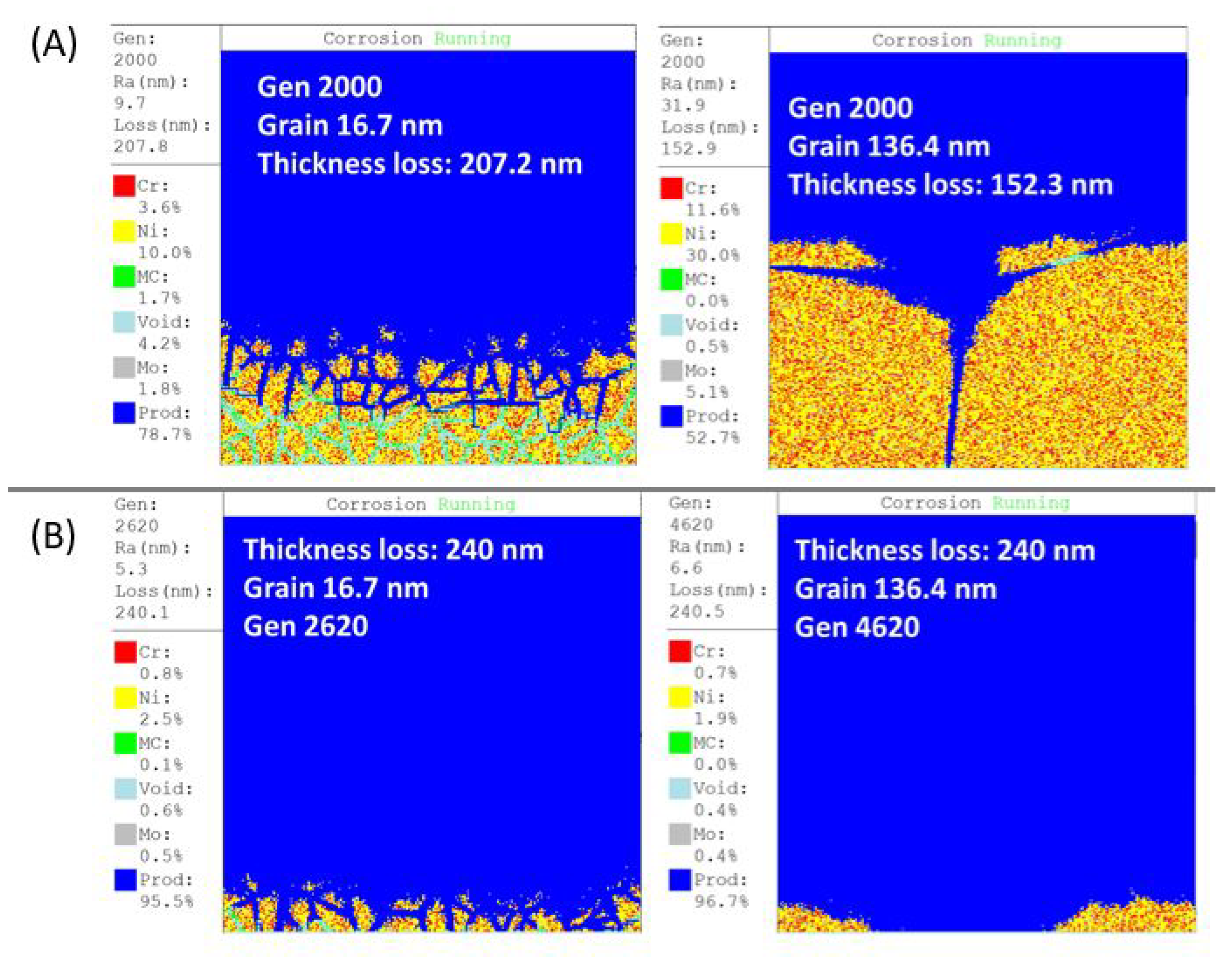
3.1. User Interface

Input cards allow the user to establish and tune the initial conditions and simulation parameters: (i) Materials card, (ii) Initboard card, (iii) Reaction card, (iv) Diffusion card, and (v) Termination criteria card. Users can control and interact with the program during simulation with keyboard commands. A GUI (graphic user interface) displays the current simulation status. As demonstrated by Figure 6, the GUI provides two display modes: diffusion and corrosion. In the top center of the window, the display mode and current status (running or paused) of the simulation are displayed. Figure 6A demonstrates the diffusion of chlorine with the status of “PAUSED”, while Figure 6B shows the corrosion process with the status of “RUNNING”. The left panel is split into two sections, with the upper section displaying the number of generations and alloy status (surface roughness and thickness loss). In diffusion mode, the lower section displays a list of color bars denoting the counts of the corrosive agent. While in the corrosion mode, it displays the materials in the grid, with each material assigned a color followed by the percent composition (at.%).

3.2. Thickness Loss

Figure 7 below compares thickness loss evolution by grain size for each of the five grain sizes used in the simulation, computed every ten generations. As the simulation terminates when the remaining material thickness is ≤10 nm, the total loss is considered equal, with the number of generations being variable. Note that the simulation with smaller grain size terminates earlier, thus indicating a greater corrosion rate.

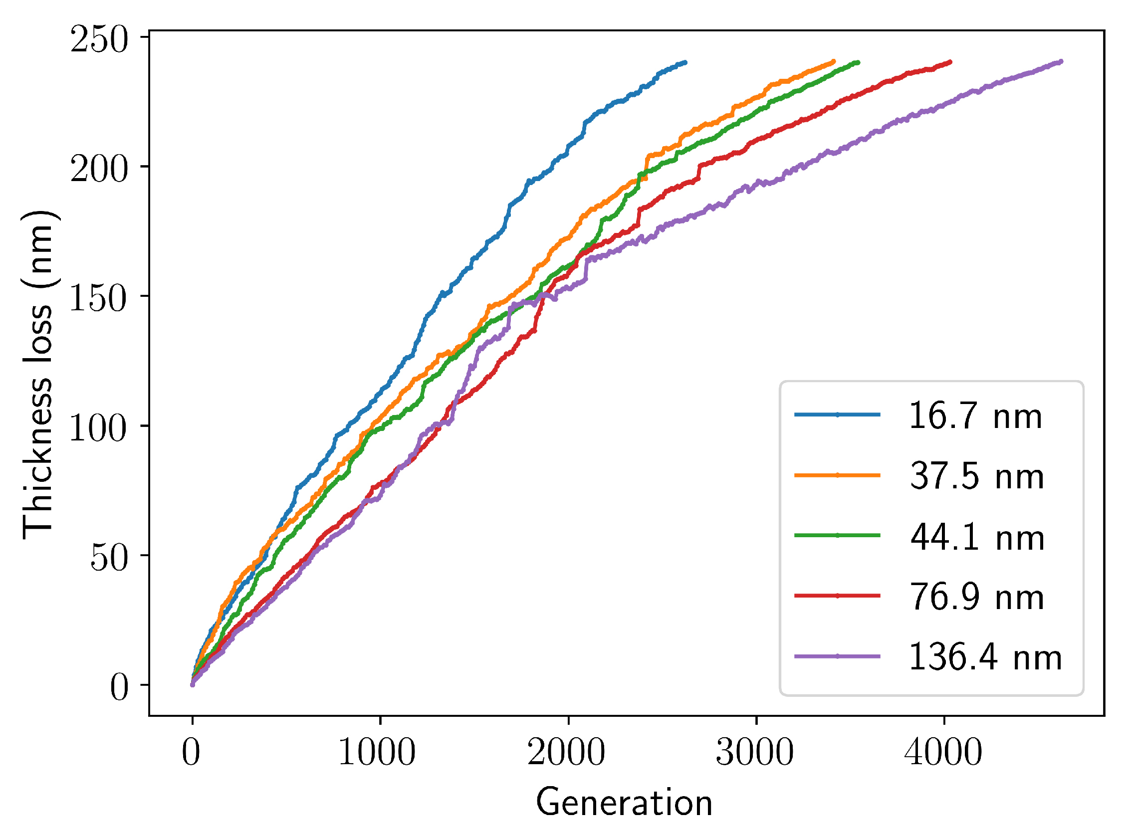
Figure 8 further demonstrates the difference in corrosion rate between the largest and smallest grain sizes. After 2000 generations, the 16.7 nm grain exhibits a thickness loss $35\%$ greater than that of the 152.3 nm grain (Figure 8A) and reaches 240 nm loss $76\%$ faster (Figure 8B).

The results above suggest that corrosion resistance increases with increasing grain size. Surface oxide passive films provide limited protection against corrosion, and are insufficient to compensate for the increased grain boundary density of smaller grain sizes, providing more corrosion initiation sites. These simulation results corroborate empirical observations detailed in previous work, in which the corrosion resistance of samples with varying grain sizes was assessed [25]. The reasons behind it are twofold: (i) limited oxide thickness (∼2 nm) [21]; (ii) oxide mainly being formed by NiO, which is less corrosion-resistant compared to Cr${ }_2$O${ }_3$ [26].

Ferguson et al. found that the type and structure of the surface oxide layers is closely related to the oxidation temperature [27]. NiO and Cr${ }_2$O${ }_3$ grow simultaneously on the surface of Inconel 625. NiO is predominant at lower temperatures, while the oxide film consists of almost entirely Cr${ }_2$O${ }_3$ at higher temperatures (between 1073 and 1323 K) [28]. In our simulation, only a NiO layer is considered for Inconel 625 without prior heat treatment.

3.3. Roughness

The surface roughness for each grain size is also logged every ten generations; the results are displayed in Figure 9. The alloy with larger grain size tends to have larger roughness and reach its peak at a larger generation. Surface roughness increases over the first half of the curve, then decrease gradually with all grain sizes exhibiting similar roughness at the end. The descending trend is attributed to the thin alloy left at large generations. Additionally, the presence of multiple large fluctuations can be observed in each condition.

The sharp increase is caused by the corrosion path along the vertical grain boundary. As shown in Figure 10, corrosion proceeds along three long vertical grain boundaries, generating three crevices. Each vertical crevice contributes a significant amount to the roughness by generating two surfaces with large deviation from average surface position. This effect is measured by the sharp rise in the orange curve between generation 0 and ∼400 in Figure 9.

As corrosion (generations) progresses, the sudden drop in roughness is attributed to the separation of a grain from the bulk alloy. This phenomenon can be observed in Figure 11, in which two grains from the 77 nm condition can be seen to separate at generation 1950 and 2050, respectively. The detached grain typically has a rough surface but no longer contributes to the alloy roughness calculation, causing the decline in the red curve in Figure 9.

3.4. Future Work

The parameters, such as diffusion coefficients and reaction rates, in the current CA program are primarily established based on literature results, and not all potential reactions are incorporated. The CA program was designed to facilitate the addition of more reactants and products, either by adding minor alloying constituents, adding minor chemical potentials, or adding additional corrosive reactants. Calibration experiments can be performed to fine-tune these parameters. Machine learning methods could also be incorporated into the program for faster and more precise parameter assessment. In addition, the program can be extended to three-dimensional geometry to better represent the realistic environment.

Currently, there is no associative time scale for simulation results compared to empirical evidence; further targeted corrosion studies coupled with the aforementioned machine learning techniques may be able to fill this void.

This tool has been developed to serve as an efficient and versatile tool for researchers to tailor to their specific alloys and environments. We believe this simulation tool can provide valuable insight into material performance in challenging environments. Using any combination of empirical and theoretical parameters, users can save valuable resources by tuning compositions and sample fabrication methods to yield grain sizes most suited to the environment at hand.

References

- Ding, W.; Bonk, A.; Bauer, T. Corrosion behavior of metallic alloys in molten chloride salts for thermal energy storage in concentrated solar power plants: A review. Front. Chem. Sci. Eng. 2018, 12, 564–576. [Google Scholar] [CrossRef]
- Williams, D.F. Assessment of Candidate Molten Salt Coolants for the NGNP/NHI Heat-Transfer Loop; Oak Ridge National Laboratory: Oak Ridge, TN, USA, 2006. [Google Scholar]
- Pragnya, P.; Gall, D.; Hull, R. In situ transmission electron microscopy of high-temperature Inconel-625 corrosion by molten chloride salts. J. Electrochem. Soc. 2021, 168, 51507. [Google Scholar] [CrossRef]
- Sun, H.; Wang, J.; Li, Z.; Zhang, P.; Su, X. Corrosion behavior of 316SS and Ni-based alloys in a ternary NaCl-KCl-MgCl2 molten salt. Sol. Energy 2018, 171, 320–329. [Google Scholar] [CrossRef]
- Liu, B.; Wei, X.; Wang, W.; Lu, J.; Ding, J. Corrosion behavior of Ni-based alloys in molten NaCl-CaCl2-MgCl2 eutectic salt for concentrating solar power. Sol. Energy Mater. Sol. Cells 2017, 170, 77–86. [Google Scholar] [CrossRef]
- Ravi Shankar, A.; Thyagarajan, K.; Kamachi Mudali, U. Corrosion behavior of candidate materials in molten LiCl-KCl salt under argon atmosphere. Corrosion 2013, 69, 655–665. [Google Scholar] [CrossRef]
- Cho, S.H.; Oh, S.C.; Park, S.B.; Ku, K.M.; Lee, J.H.; Hur, J.M.; Lee, H.S. High temperature corrosion behavior of Ni-based alloys. Met. Mater. Int. 2012, 18, 939–949. [Google Scholar] [CrossRef]
- Kondo, M.; Nagasaka, T.; Muroga, T.; Sagara, A.; Noda, N.; Xu, Q.; Ninomiya, D.; Masaru, N.; Suzuki, A.; Terai, T. High performance corrosion resistance of nickel-based alloys in molten salt flibe. Fusion Sci. Technol. 2009, 56, 190–194. [Google Scholar] [CrossRef]
- Ralston, K.D.; Birbilis, N. Effect of Grain Size on Corrosion: A Review. Corrosion 2010, 66, 075005. [Google Scholar] [CrossRef]
- Pérez-Brokate, C.F.; Di Caprio, D.; Féron, D.; De Lamare, J.; Chaussé, A. Overview of Cellular Automaton Models for Corrosion; Springer: Berlin/Heidelberg, Germany, 2014; pp. 187–196. [Google Scholar]
- Menshutina, N.V.; Kolnoochenko, A.V.; Lebedev, E.A. Cellular automata in chemistry and chemical engineering. Annu. Rev. Chem. Biomol. Eng. 2020, 11, 87–108. [Google Scholar] [CrossRef]
- Svyetlichnyy, D.S. A three-dimensional frontal cellular automaton model for simulation of microstructure evolution—Initial microstructure module. Model. Simul. Mater. Sci. Eng. 2014, 22, 1–19. [Google Scholar] [CrossRef]
- Demontis, P.; Pazzona, F.G.; Suffritti, G.B. A lattice-gas cellular automaton to model diffusion in restricted geometries. J. Phys. Chem. B 2006, 110, 13554–13559. [Google Scholar] [CrossRef]
- Bandman, O.L. A cellular automata convection-diffusion model of flows through porous media. Optoelectron. Instrum. Data Process. 2007, 43, 524–529. [Google Scholar] [CrossRef]
- Kireeva, A. Two-layer CA for simulation of catalytic reaction at dynamically varying surface temperature. J. Comput. Sci. 2015, 11, 317–325. [Google Scholar] [CrossRef]
- Scalise, D.; Schulman, R. Emulating cellular automata in chemical reaction-diffusion networks. Nat. Comput. 2016, 15, 197–214. [Google Scholar] [CrossRef]
- Bandman, O. A Hybrid Approach to Reaction-Diffusion Processes Simulation; Springer: Berlin/Heidelberg, Germany, 2001; pp. 1–16. [Google Scholar]
- Van der Weeën, P. Meso-Scale Modeling of Reaction-Diffusion Processes using Cellular Automata. Ph.D. Thesis, University of Ghent, Ghent, Belgium, 2014. [Google Scholar]
- Mai, J.; Kuzovkov, V.N.; von Niessen, W. Stochastic model for the A+B2 surface reaction: Island formation and complete segregation. J. Chem. Phys. 1994, 100, 6073–6081. [Google Scholar] [CrossRef]
- Chopard, B.; Droz, M. Cellular Automata; Springer: Berlin/Heidelberg, Germany, 1998; Volume 1, pp. 139–150. [Google Scholar]
- Feng, J.; Yuan, G.; Mao, L.; Leão, J.B.; Bedell, R.; Ramic, K.; de Stefanis, E.; Zhao, Y.; Vidal, J.; Liu, L. Probing layered structure of Inconel 625 coatings prepared by magnetron sputtering. Surf. Coat. Technol. 2021, 405, 126545. [Google Scholar] [CrossRef] [PubMed]
- Smithells, C.J.; Ransley, C.E. The diffusion of gases through metals-IV—The diffusion of oxygen and of hydrogen through nickel at very high pressures. Proc. R. Soc. Lond. Ser. A-Math. Phys. Sci. 1936, 157, 292–302. [Google Scholar]
- Cussler, E.L.; Cussler, E.L. Diffusion: Mass Transfer in Fluid Systems; Cambridge University Press: Cambridge, UK, 2009. [Google Scholar]
- Askill, J. Tracer Diffusion Data for Metals, Alloys, and Simple Oxides; Springer Science & Business Media: Berlin/Heidelberg, Germany, 2012. [Google Scholar]
- Feng, J.; Mao, L.; Yuan, G.; Zhao, Y.; Vidal, J.; Liu, L.E. Grain size effect on corrosion behavior of Inconel 625 film against molten MgCl2-NaCl-KCl salt. Corros. Sci. 2022, 197, 110097. [Google Scholar] [CrossRef]
- Sugimoto, K.; Seto, M.; Tanaka, S.; Hara, N. Corrosion resistance of artificial passivation films of Fe2O3-Cr2O3-NiO formed by metalorganic chemical vapor deposition. J. Electrochem. Soc. 1993, 140, 1586. [Google Scholar] [CrossRef]
- Ferguson, J.B.; Lopez, H.F. Oxidation products of Inconel alloys 600 and 690 in pressurized water reactor environments and their role in intergranular stress corrosion cracking. Metall. Mater. Trans. A 2006, 37, 2471–2479. [Google Scholar] [CrossRef]
- Kumar, L.; Venkataramani, R.; Sundararaman, M.; Mukhopadhyay, P.; Garg, S.P. Studies on the oxidation behavior of Inconel 625 between 873 and 1523 K. Oxid. Met. 1996, 45, 221–244. [Google Scholar] [CrossRef]
- Feng, J. Study on the Corrosion Behavior of Inconel 625 in Molten Chloride Salt. Ph.D. Thesis, Rensselaer Polytechnic Institute, Troy, NY, USA, 2021. Available online: https://www.proquest.com/docview/2729021274?pq-origsite=gscholar&fromopenview=true&sourcetype=Dissertations%20&%20Theses (accessed on 24 July 2024).
Disclaimer/Publisher’s Note: The statements, opinions and data contained in all publications are solely those of the individual author(s) and contributor(s) and not of MDPI and/or the editor(s). MDPI and/or the editor(s) disclaim responsibility for any injury to people or property resulting from any ideas, methods, instructions or products referred to in the content. |
© 2024 by the authors. Licensee MDPI, Basel, Switzerland. This article is an open access article distributed under the terms and conditions of the Creative Commons Attribution (CC BY) license (https://creativecommons.org/licenses/by/4.0/).
Share and Cite
Feng, J.; Gao, J.; Mao, L.; Bedell, R.; Liu, E. Modeling the Impact of Grain Size on Corrosion Behavior of Ni-Based Alloys in Molten Chloride Salt via Cellular Automata. Metals 2024, 14, 931. https://doi.org/10.3390/met14080931
Feng J, Gao J, Mao L, Bedell R, Liu E. Modeling the Impact of Grain Size on Corrosion Behavior of Ni-Based Alloys in Molten Chloride Salt via Cellular Automata. Metals. 2024; 14(8):931. https://doi.org/10.3390/met14080931
Chicago/Turabian StyleFeng, Jinghua, Jianxi Gao, Li Mao, Ryan Bedell, and Emily Liu. 2024. "Modeling the Impact of Grain Size on Corrosion Behavior of Ni-Based Alloys in Molten Chloride Salt via Cellular Automata" Metals 14, no. 8: 931. https://doi.org/10.3390/met14080931
APA StyleFeng, J., Gao, J., Mao, L., Bedell, R., & Liu, E. (2024). Modeling the Impact of Grain Size on Corrosion Behavior of Ni-Based Alloys in Molten Chloride Salt via Cellular Automata. Metals, 14(8), 931. https://doi.org/10.3390/met14080931