Rapid Assessment of Steel Machinability through Spark Analysis and Data-Mining Techniques

Abstract

The machinability of steel is a crucial factor in manufacturing, influencing tool life, cutting forces, surface finish, and production costs. Traditional machinability assessments are labor-intensive and costly. This study presents a novel methodology to rapidly determine steel machinability using spark testing and convolutional neural networks (CNNs). We evaluated 45 steel samples, including various low-alloy and high-alloy steels, with most samples being calcium steels known for their superior machinability. Grinding experiments were conducted using a CNC machine with a ceramic grinding wheel under controlled conditions to ensure a constant cutting force. Spark images captured during grinding were analyzed using CNN models with the ResNet18 architecture to predict V15 values, which were measured using the standard ISO 3685 test. Our results demonstrate that the created prediction models achieved a mean absolute percentage error (MAPE) of 12.88%. While some samples exhibited high MAPE values, the method overall provided accurate machinability predictions. Compared to the standard ISO test, which takes several hours to complete, our method is significantly faster, taking only a few minutes. This study highlights the potential for a cost-effective and time-efficient alternative testing method, thereby supporting improved manufacturing processes.

1. Introduction

The term machinability refers to the relative ease or difficulty with which a material can be machined, indicating how easily or challenging it is to shape a workpiece using the appropriate cutting tools and parameters [1]. This definition applies to all mechanical material processing involving cutting. Since machinability is a specific technological property of a material, it cannot be easily linked to the unique properties of the work material. It is considered a resultant property of the machining system, influenced by factors such as the mechanical and physical properties of the work material, tool material and geometry, type of machining process, clamping system, coolant, and cutting parameters [2].

Generally, factors that improve the basic properties of a material, such as strength and hardness, often degrade its machinability [3]. Currently, machinability is evaluated using several parameters, the most important being tool life or wear rate, cutting forces or energy consumption during machining, surface quality of the machined part, maximum cutting speed, and chip formation [4]. Engineering materials are thus classified into two categories: easily machinable and difficult-to-machine materials. Easily machinable materials are characterized by their ability to facilitate faster cutting speeds, reduced cutting forces and power consumption, better surface quality, and extended tool life [5]. In contrast, difficult-to-machine materials require greater cutting forces, exhibit higher tool wear rates, and often result in poor surface quality, thereby increasing the overall cost and time of the machining process [6]. This distinction is vital for selecting appropriate materials for specific engineering applications, especially in high-precision and high-efficiency manufacturing environments.

In our research, we focus on the machinability of low-alloy steels and low-alloy steels with improved machinability. The incorporation of certain alloying elements such as sulfur and calcium in low-alloy steels has been shown to significantly improve their machinability [6]. These steels exhibit a significantly longer tool life even at higher cutting speeds. Despite the manufacturing costs of improved machinability steels being comparable to conventional steels, their prices can be up to 15% higher [3]. Experiments have shown that improved machinability can achieve machining at 25–50% higher cutting speeds, reduce tool wear by 4 to 6 times, and lower machining costs by 30%, while other properties of the steel remain unchanged [7].

Predicting machinability is generally difficult due to the numerous variables associated with the production (e.g., casting macrostructure, microstructure, heat treatment, and postprocessing) and machining process (e.g., machining type, machining parameters, part geometry, etc.) [8]. The complexity of these factors makes it difficult to develop accurate and reliable predictions for machinability. Therefore, enhancing the technical capabilities to predict machinability is crucial for modern manufacturing.

Machinability tests are categorized into ranking tests and absolute tests, with absolute tests providing a more comprehensive picture of machining characteristics. The most commonly used absolute test for determining steel machinability is conducted according to ISO 3685 [9]. Additionally, ISO 8688 provides guidelines for the tool life testing of end mills and face mills, further contributing to the comprehensive evaluation of machinability [10,11]. Both standards are crucial for establishing consistent and reliable measures of machinability across different steel grades and machining processes. However, this test is time-consuming, labor-intensive, and costly, posing significant challenges in industries where precise knowledge of steel machinability is essential. Without machinability data, steel cannot proceed to subsequent technological processes. The chemical composition, inclusions (size, shape, and distribution), and microstructure complicate machinability predictions, further affected by the varying technological parameters of steel production [12]. In recent years, researchers have invested considerable effort into developing short absolute tests that enable the rapid and cost-effective determination of steel machinability.

Researchers have developed mathematical models for predicting steel machinability based on the surface quality, tool wear, and cutting forces during turning [13,14]. Šalak et al. [15] developed a method for the rapid determination of machinability during turning using smaller diameter test samples in their research. Several methods have been developed that use turning to predict the tool life and, consequently, the machinability. Šalak et al. [16] investigated the machinability of powder metallurgy steels, focusing on the influence of various alloying elements and sintering processes on tool wear and cutting efficiency. Békés [17] explored the engineering technology involved in the machining of metals, providing insights into the optimization of cutting parameters for enhanced tool life and surface quality. Jakubéczyová and Fáberová [18] examined the mechanical properties and surface treatment effects on PM cobalt high-speed steels, highlighting the role of surface coatings in extending tool life during high-speed machining. Ebrahimi and Moshksar [19] conducted an evaluation of machinability in turning micro-alloyed and quenched-tempered steels, utilizing statistical analysis and chip morphology to correlate tool wear with cutting performance and material properties. Several methods for determining the machinability of steels have also been developed using the drilling process. In one study [20], machinability was assessed for three different types of steel by measuring drill wear. Blais et al. [21] assessed the machinability of sintered steels using drilling operations by measuring cutting forces, tool wear, and surface roughness. Most of the aforementioned methods for assessing machinability during turning or drilling can only be applied to specific steel types or do not rely on absolute machinability tests. Consequently, their results cannot be directly compared to the standard absolute test, where machinability is expressed as the cutting speed at which the tool wears out after 15 min of machining. Determining machinability through turning and drilling poses a significant challenge for companies, mainly due to the high consumption of cutting tools and the resulting high costs of tool procurement.

Given these limitations, the idea arises to use another machining process for rapid machinability assessment. The literature lacks studies utilizing the grinding process to determine steel machinability. Grinding, mainly a fine machining process, involves undefined cutting geometry tools and generates sparks due to high material deformation and heat release [22]. Spark characteristics during grinding provide extensive information about the process and material [23]. Researchers have analyzed spark characteristics to determine material removal rates [24,25,26], optimal grinding conditions [27], grinding wheel life [28], and carbon content in steel [29,30,31]. However, no studies have used spark characteristics to determine steel machinability.

This paper presents a novel methodology for determining steel machinability based on spark data during grinding. An experimental setup involving grinding and machine vision will be introduced to capture and analyze spark images. These images will be used to develop convolutional neural network (CNN) models for predicting steel machinability. The paper will detail the experimental setup, image processing methodology, and CNN model development, followed by a thorough analysis of the obtained results.

2. Materials and Methods

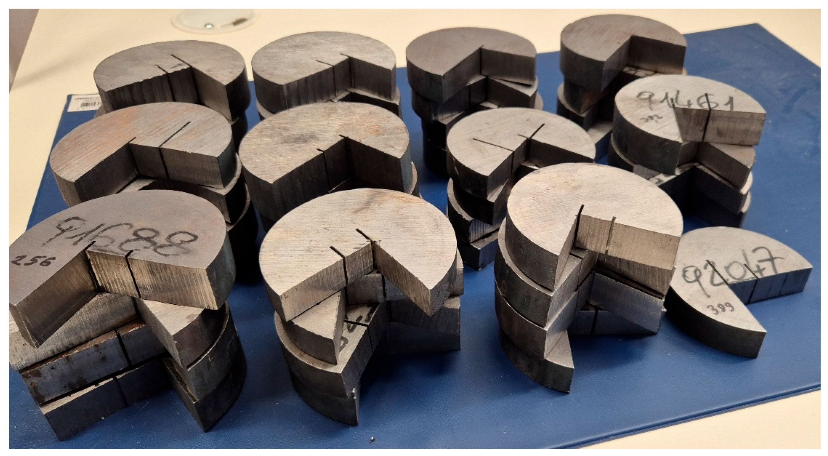
2.1. Steel Samples

In this study, 45 different steel samples were used to evaluate machinability based on spark testing. These samples included multiple instances of steels with identical chemical compositions but varying machinability and hardness due to different production times. The chemical compositions of the samples included 16MnCrS5, 16NiCrS4, 20MnV6, 30CrNiMo8, 34CrNiMo6, 38MnVS6, 42CrMoS4, and C45. All samples were sourced from Štore Steel Ltd. (Štore, Slovenia). Additionally, most of the samples were calcium-treated steels [32], which are known for their exceptional machinability and consistent quality. The selected steel grades encompass a range of low-alloy and high-alloy steels, chosen for their relevance in manufacturing and their varying machinability characteristics. Some samples had the same chemical composition but exhibited different machinability and hardness due to differing production conditions.

To ensure consistency and reliability in the experimental results, the chemical compositions of each sample were verified using spectroscopic analysis, and mechanical properties such as hardness were measured according to standard procedures. Machinability values were obtained using the standard machinability test based on ISO 3685 [9]. This internationally recognized standard specifies a comprehensive procedure for tool life testing with single-point turning tools, aimed at providing reliable and consistent measurements of machinability. The test is known to be time-consuming and costly due to its extensive and meticulous nature. The ISO 3685 [9] test involves a series of systematic steps to evaluate tool life under controlled conditions. Initially, it requires selecting appropriate cutting tools and workpiece materials, ensuring that they meet the specified standards for the test. The procedure includes multiple iterations of tool life testing at various cutting speeds to accurately plot the tool life curve. This curve is essential for determining the relationship between cutting speed and tool life, which is a critical aspect of machinability assessment. To achieve this, the test requires significant machine time, labor, and consumable resources. Each iteration involves running the cutting tool at a set speed until a predefined criterion of tool wear is reached, typically measured by flank wear or crater wear. These iterations must be repeated at different speeds to cover a range of cutting conditions. The resulting data are used to construct the tool life curve, from which the machinability rating is derived.

The Taylor equation, which relates tool life ($t$) to cutting speed ($v$), is used to determine the machinability rating. The equation is expressed as:

$$v{t}^n=C,$$

(1)

where $v$ is the cutting speed in meters per minute, $t$ is the tool life, $n$ is the tool life exponent (a constant that depends on the tool and workpiece material), and $C$ is a constant for a given tool–material combination. For the ISO 3685 standard [9], a specific value known as V15 is often calculated. V15 represents the cutting speed at which the tool life is 15 min and it is typically measured in meters per minute (m/min). This value is determined from the tool life curve plotted during the tests. The V15 value provides a standardized measure of machinability, allowing for comparison between different materials.

In our study, the V15 machinability of our steel samples was assessed at Štore Steel steel plant using the standard ISO 3685 test [9]. The test demands precise control and measurement of cutting conditions, such as cutting speed, feed rate, and depth of cut, to ensure reproducible and accurate results. This includes maintaining constant conditions throughout each test run and accurately measuring the wear on the cutting tools. The complexity and expense of the procedure are further increased by the need for specialized equipment and skilled personnel to conduct the tests and analyze the results.

Table 1. Steel samples.

Sample Index	Heat	Quality	HBW	V15 [m/min]	Machining Time [min]
1	92369	42CrMoS4	180	299	14.87
2	93137	16MnCrS5	143	411	15.12
3	93541	42CrMoS4	280	207	14.10
4	92047	C45	186	389	20.56
5	92718	16MnCrS5	151	416	15.83
6	92249	42CrMoS4	257	229	21.25
7	92456	C45	151	377	18.03
8	92331	20MnV6	210	411	16.66
9	92145	20MnV6	199	401	15.19
10	92796	42CrMoS4	198	236	23.98
11	91678	C45	190	385	19.71
12	91688	30CrNiMo8	210	256	16.50
13	92330	20MnV6	206	405	15.73
14	93511	C45	192	384	19.36
15	93677	C45	189	382	18.97
16	93706	34CrNiMo6	206	266	16.55
17	91461	C45/75	187	382	18.97
18	93644	C45/75	183	374	17.48
19	93516	16MnCrS5	151	423	17.00
20	92147	16MnCrS5	157	433	18.76
21	91959	C45	184	393	21.37
22	92613	16NiCrS4	189	476	18.78
23	92251	16MnCrS5	144	418	16.27
24	91958	C45	192	374	17.48
25	91943	16MnCrS5	154	429	18.06
26	93648	42CrMoS4	212	227	20.49
27	91792	20MnV6	206	360	9.82
28	92623	20MnV6	206	401	15.19
29	92328	20MnV6	208	397	14.61
30	93696	34CrNiMo6	226	271	17.72
31	93647	42CrMoS4	276	222	18.71
32	92252	16MnCrS5	152	423	17.00
33	92329	20MnV6	202	405	15.73
34	93746	16MnCrS5	158	423	17.00
35	92065	20MnV6	202	408	16.22
36	93802	16MnCrS5	153	437	19.44
37	92715	42CrMoS4	214	229	21.25
38	93518	16MnCrS5	156	433	18.76
39	93873	34CrNiMo6	209	266	16.55
40	91721	38MnVS6	277	249	14.85
41	91724	C45	194	374	17.48
42	91942	16MnCrS5	155	421	16.66
43	92624	20MnV6	207	408	16.22
44	92412	C45	213	374	17.48
45	92781	42CrMoS4	209	239	25.36

summarizes the detailed information of each steel sample, including heat number, quality, HBW hardness, machinability (V15), and machining time, during the machinability test.

A photograph of the steel samples is included in Figure 1, illustrating the variety and consistency of the samples used in this study. The samples had irregular shapes, as they were remnants from different tests conducted at the steel plant.

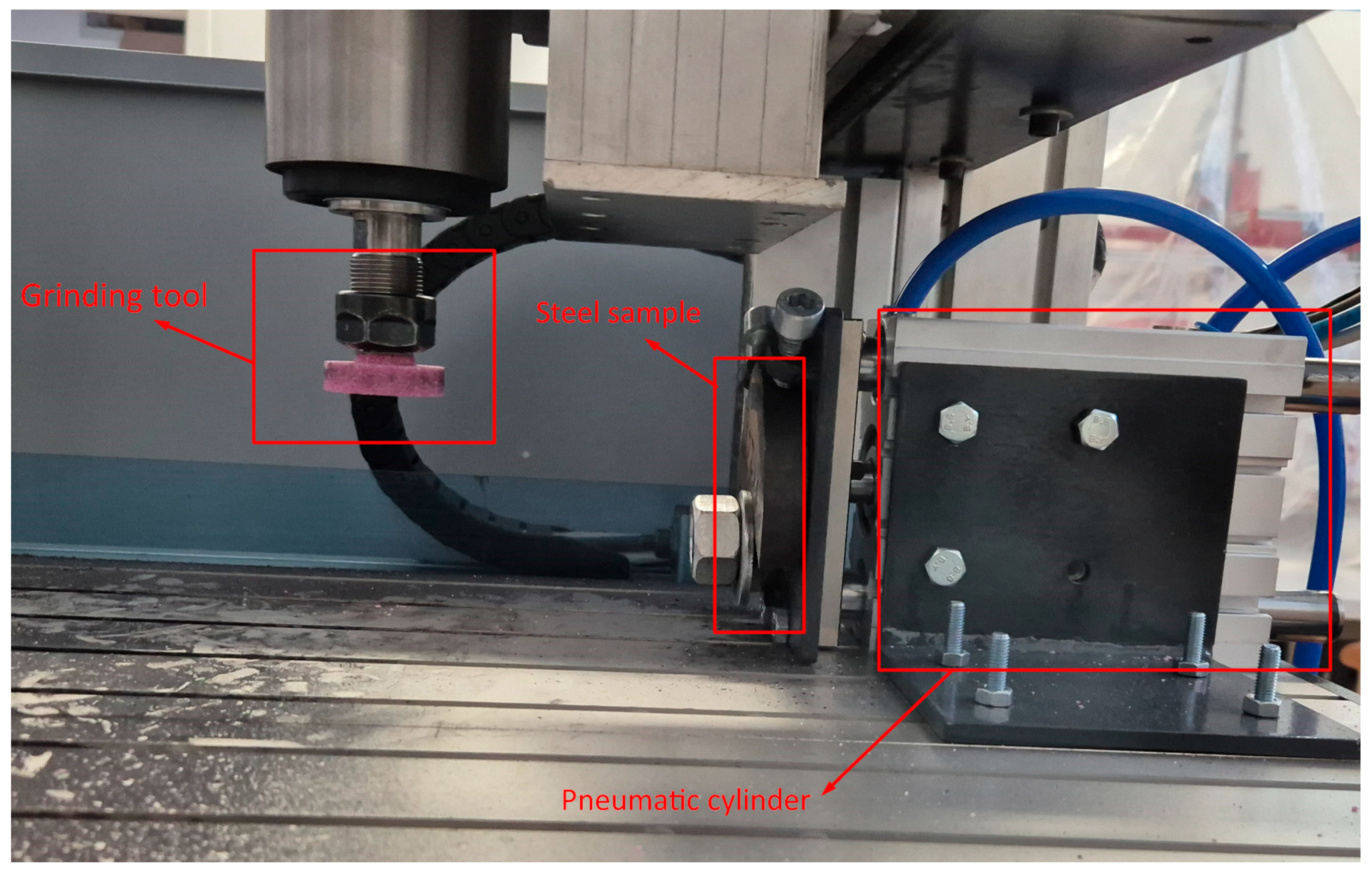
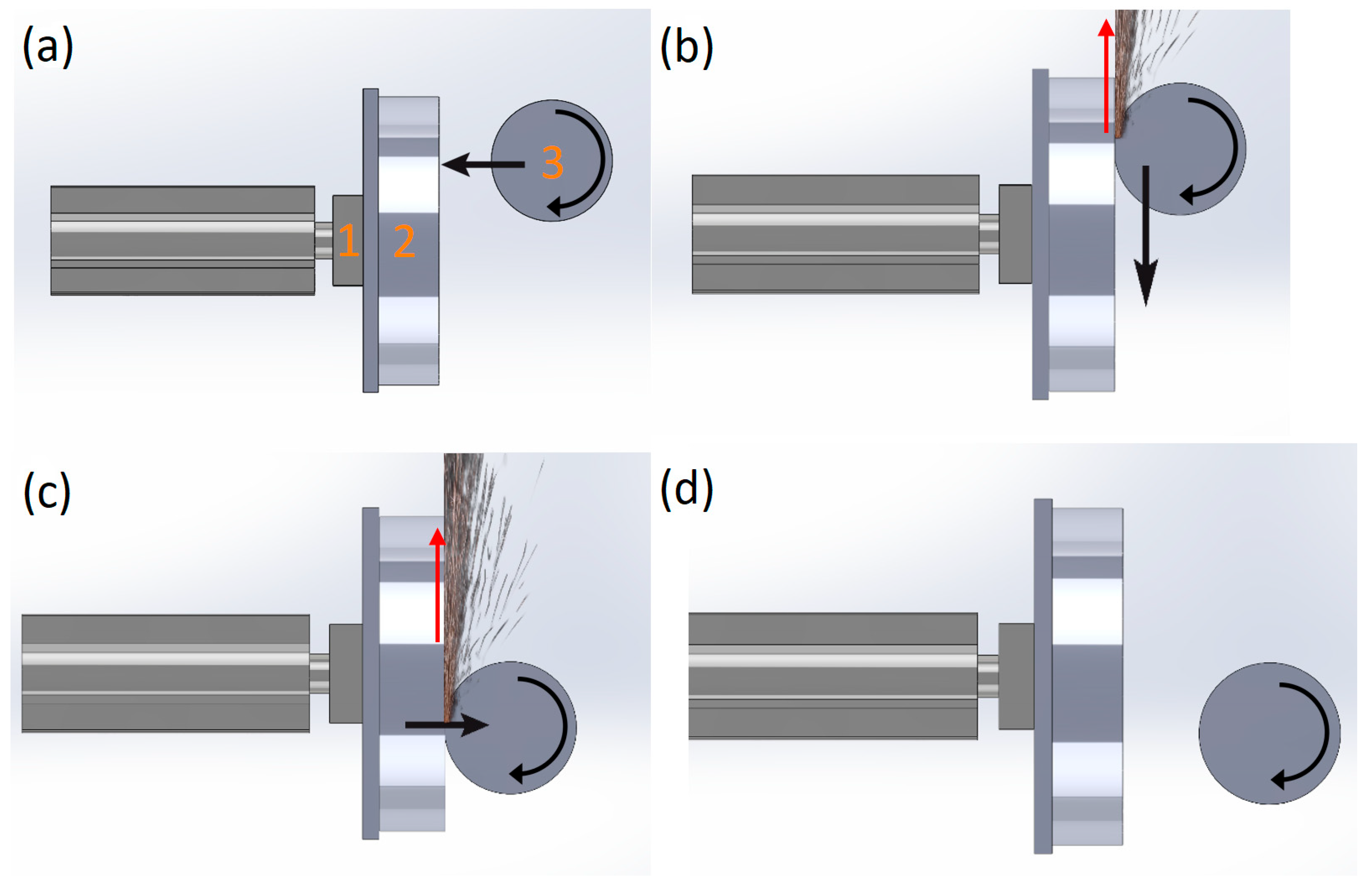
2.2. Experimental Setup

The grinding experiment on steel samples was conducted using a smaller custom-made CNC machine. The tool used for the experiment was a ceramic grinding wheel designed for steel and cast iron. The grinding wheel was cylindrical, with a diameter of 40 mm, a height of 10 mm, and a grit size of K30. This tool was chosen for its excellent performance in both rough and fine grinding of structural steel, cast iron, and machine steels, as well as its effectiveness in grinding harder materials. Using this tool, we were able to generate a sufficient number of sparks for analysis.

The experiment was designed to maintain a constant cutting force during grinding. This was achieved using a pneumatic cylinder with a diameter of 30 mm, connected to an Enfield TR-010-g10-s (Enfield Technologies, Trumbull, CT, USA) proportional electro-pneumatic pressure regulator. This regulator was selected for its high regulation speed (2.5 ms) and accuracy (±0.1%). The experimental setup is illustrated in Figure 2.

To ensure a constant cutting force during grinding, a constant pressure of 0.6 bar was maintained in the pneumatic cylinder. The cutting force used during the experiment was calculated based on the diameter of the pneumatic cylinder and the regulated pressure. Specifically, the cutting force was determined by using a 40 mm-diameter pneumatic SGM 40/100 cylinder (E·MC Pneumatics, Ningbo, China) and applying the regulated pressure of 0.6 bar. This setup resulted in a cutting force of 75.4 N, which was maintained consistently throughout the experiment.

The grinding experiment was conducted by feeding the tool into the steel sample, which was mounted on the pneumatic cylinder, ensuring a constant pressure and, consequently, a constant cutting force.

Figure 3 illustrates the schematic of the grinding experiment. In Figure 3a, the initial position of the experiment is depicted, where number 1 represents the piston of the pneumatic cylinder, number 2 denotes the steel sample, and number 3 indicates the grinding tool. The straight arrow shows the direction of tool movement, while the curved arrow indicates the tool’s rotational direction. The tool first moves towards the steel sample until contact is made. The start of grinding is shown in Figure 3b. The tool then begins to move longitudinally along the sample, producing sparks. The direction of the sparks generated during grinding is indicated by the red arrow. Figure 3c illustrates the end of the grinding process, where the tool starts to move away from the sample. Sparks continue to be generated until the tool loses contact with the sample. Figure 3d shows the conclusion of the experiment, where the tool has left the steel sample and no more sparks are produced. Spark images were captured while the tool moved longitudinally along the sample (starting from the position shown in Figure 3b and ending at the position shown in Figure 3c). This approach eliminated disturbances that occur at the beginning and end of the grinding process when the tool is not fully in contact with the steel sample.

The cutting parameters during the experiment were as follows:

• Rotational speed of the grinding wheel: 400 RPM;
• Feed rate: 250 mm/s;
• Cutting length: 15 mm.

Using these cutting parameters, the experiment was performed four times for each steel sample. This ensured that each sample was ground long enough to obtain a sufficient number of spark images using the machine vision system, which will be described in the next section.

To ensure the reproducibility of the experiments, all equipment was calibrated before use and each grinding test was repeated four times per sample. The spark images were recorded meticulously to facilitate accurate analysis and validation of the results.

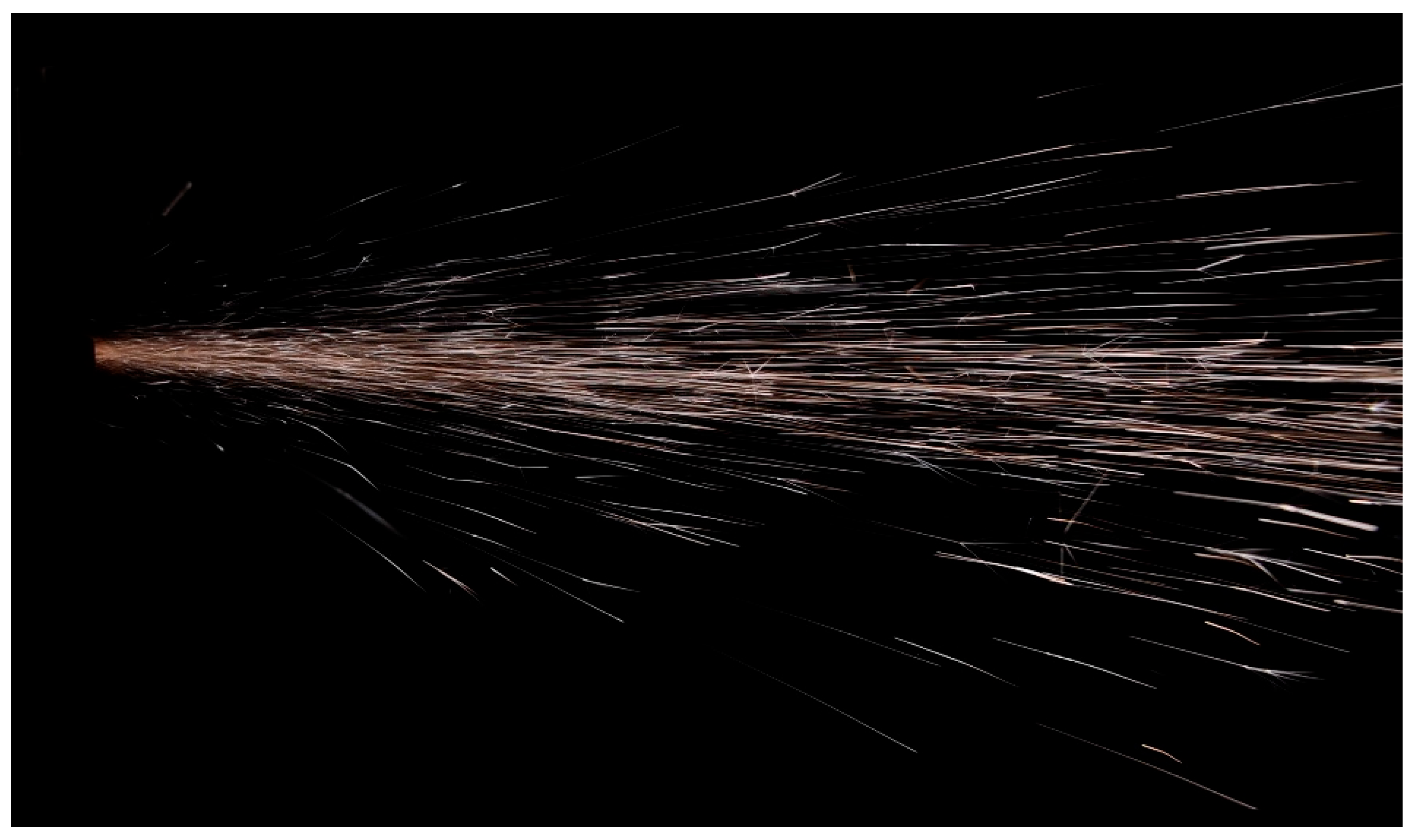
2.3. Machine Vision System

The machine vision system used in this study is designed to capture and analyze the characteristics of sparks generated during the grinding process. The system comprises a high-speed camera and data acquisition hardware, specifically configured to ensure accurate and detailed imaging of the sparks.

A Nikon D90 professional camera with a 23 mm-focal-length lens was used to capture the spark images during experiment. The camera was positioned behind the grinding tool, as illustrated in Figure 4, and set to capture images at a resolution of 3216 × 2136 pixels. Due to the brightness of the sparks, no additional lighting was necessary.

The camera settings were adjusted to ensure that only the sparks were visible in the images, without interference from the tool, steel sample, or background. The image capture parameters were as follows:

• Shutter Speed [s]: 1/160;
• Aperture: f/8;
• ISO Speed: 200;
• White Balance [K]: 2500.

Using the aforementioned parameters, we successfully captured clear images of the sparks, free from background disturbances. An example of the captured images is shown in Figure 5. During a single grinding cycle, approximately 20 spark images were generated. Since the experiment was repeated four times for each steel sample, around 80 spark images were obtained per sample.

To ensure the accuracy and reliability of the captured images, the camera was calibrated before each set of experiments. The captured images were then stored and organized using a dedicated data management system, facilitating easy retrieval and analysis.

The processing of the acquired images, including feature extraction and analysis, will be described in the following subsection. This setup ensured that the captured images were suitable for detailed analysis, providing a robust dataset for evaluating the machinability of the steel samples using spark characteristics.

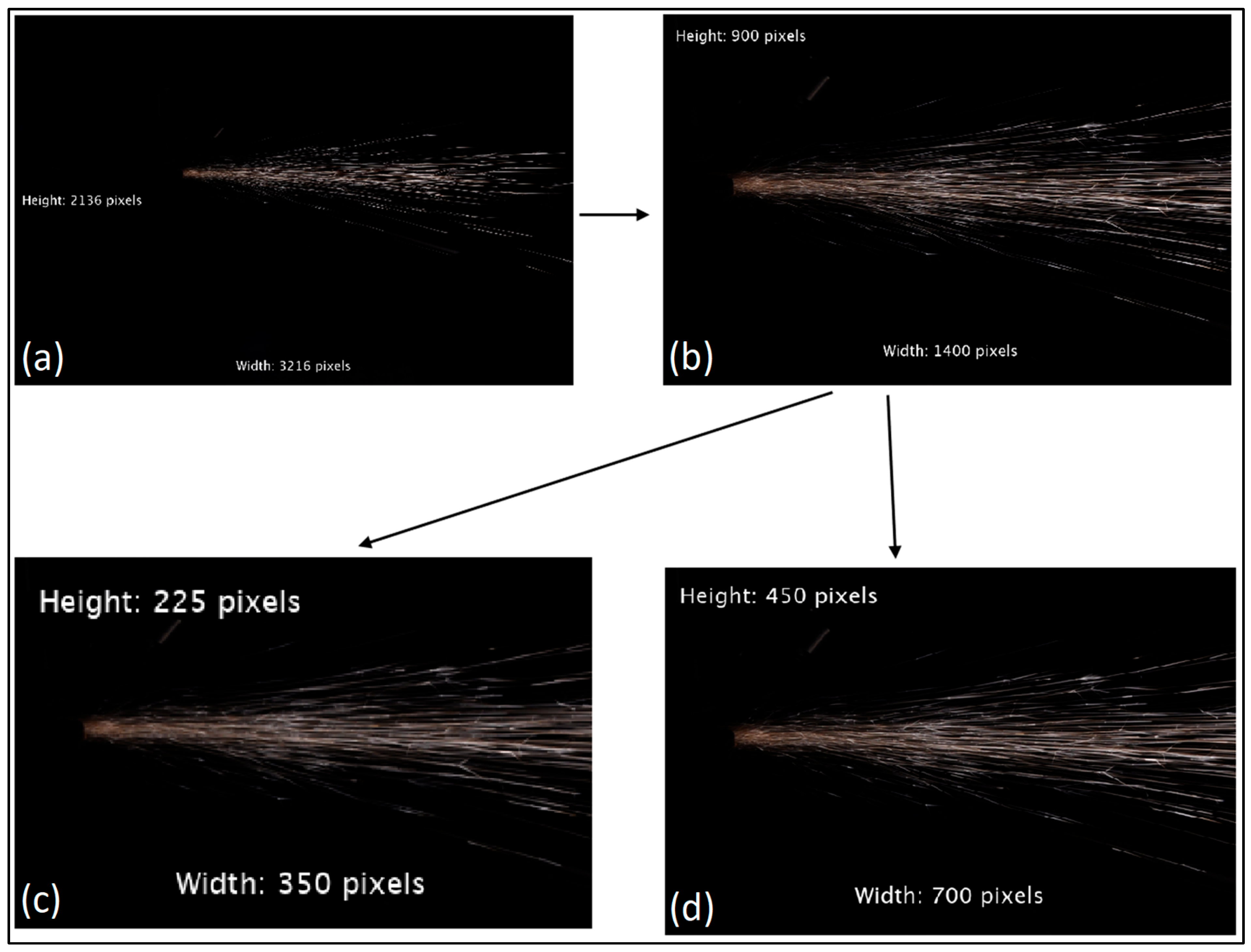
2.4. Image Preprocessing Methods

The captured images of sparks were processed using a combination of image preprocessing techniques and advanced data analysis methods.

The initial preprocessing of the images included noise reduction, contrast enhancement, and background subtraction to isolate the sparks from the rest of the image. Noise reduction and background subtraction were achieved by optimizing the camera settings. By using a sufficiently short shutter speed, we ensured that the background was not visible in the images. An example of an original image captured during the experiment is shown in Figure 6a. The original images were RGB images with a horizontal resolution of 3216 pixels and a vertical resolution of 2136 pixels.

Subsequent preprocessing was performed using MATLAB R2023b. The acquired images contained a substantial amount of dark background that did not provide any information about the steel samples. Therefore, the images were cropped to remove as much of the background as possible. The original images were cropped to retain the portion of the image from pixel 800 to pixel 2200 horizontally and from pixel 500 to pixel 1400 vertically. An example of a cropped image is shown in Figure 6b. The resulting cropped images had dimensions of 1400 pixels horizontally and 900 pixels vertically.

To ensure efficient and effective training of the models for predicting the machinability of steels, the images needed to be resized further. We aimed to determine if the image size, and, consequently, the level of detail in the images, affected the accuracy of the predictive models. Therefore, we decided to use two different image sizes: images with dimensions four times smaller and images with dimensions two times smaller than the original cropped images. The resizing was performed using MATLAB R2023b, resulting in images of two different sizes: 350 × 225 pixels, as shown in Figure 6c, and 700 × 450 pixels, as shown in Figure 6d. The processed images were then used to develop convolutional neural network (CNN) models for predicting the machinability of steels. The description and development of these models will be detailed in the next subsection.

2.5. CNNs for Machinability Prediction

In this study, we employed convolutional neural networks (CNNs) to predict the machinability of steel, based on images of sparks generated during the grinding process. CNNs are a class of deep-learning models particularly effective for image-processing tasks due to their ability to automatically and adaptively learn spatial hierarchies of features from input images [33,34].

For our study, a well-established CNN architecture, ResNet-18, was used. ResNet-18 is part of the residual network family and is renowned for its depth and ability to achieve high accuracy in image classification tasks. Introduced by He et al. [35], ResNet-18 addresses the vanishing gradient problem in deep networks by employing residual connections, which allow gradients to bypass certain layers. ResNet-18 consists of 18 layers, including convolutional, batch normalization, ReLU activation, and pooling layers. The model’s architecture is organized into residual blocks, each containing two or three convolutional layers with shortcut connections that enhance gradient flow during backpropagation. We chose ResNet-18 for its proven robustness and performance in various computer vision applications. Its ability to generalize well across different datasets and tasks makes it an ideal choice for our study, which involves predicting machinability based on images of sparks generated during grinding. The ResNet-18 architecture was implemented and trained using MATLAB R2023b, which provides a robust and flexible environment for deep-learning model development.

MATLAB’s “Deep Learning Toolbox” [36] provided us with pre-trained models and facilitated transfer learning, which is crucial for adapting pre-trained networks to new tasks with limited data. The ResNet-18 model is originally designed for classification tasks. However, to implement this architecture for our specific needs, we employed transfer-learning techniques to modify the network for regression tasks. Transfer learning involves fine-tuning a pre-trained network on a new, but related task. This approach not only leverages the powerful feature extraction capabilities of the pre-trained networks but also significantly reduces the time and computational resources required for training [37]. Using transfer learning, two different ResNet-18 models were created from pre-trained models. Specifically, we replaced the final fully connected layers of pre-trained ResNet-18 network, which are designed for classification, with new layers suitable for regression tasks. This modification allowed the networks to output continuous values representing the machinability of the steel samples, rather than discrete class labels. Additionally, we modified the first layer of each model to accept different sizes of input images. The first ResNet-18 model was modified to accept input images of size 350 × 225 pixels. For this model, we will subsequently use the label “ResNet-18_small”, as it operates using smaller-sized images. The second ResNet-18 model was modified to accept input images of size 700 × 450 pixels. For the second model, we will subsequently use the label “ResNet-18_big”, as it operates using larger-sized images.

Both networks were trained on a dataset of images captured during the grinding process, with the corresponding machinability values (V15) obtained from the standard test ISO 3685, conducted at the steel plant Štore Steel. The V15 machinability value, expressed in meters per minute (m/min), served as the target variable in our CNN models. The training process involved optimizing the weights of the networks using a suitable loss function for regression. In our study, we used root mean square error (RMSE) [38]. In our study, RMSE was used to measure the difference between the predicted V15 values and the actual V15 values from the ISO 3685 test [9]. To ensure consistency between training both models (ResNet18_small and ResNet18_big), training options were the same for both models and are listed in

Table 2. Training options.

Training Option	Value
Solver type	SGDM
Learning rate	0.000001
Mini batch size	32
Validation frequency	20
Shuffle	Every epoch

.

For solver type, we used stochastic gradient descent with momentum (SGDM), which is an optimization technique used primarily in training deep-learning models and neural networks to speed convergence [39]. SGDM enhances the basic stochastic gradient descent (SGD) algorithm by incorporating a momentum term, which helps to smooth out the oscillations in gradient descent updates, thus accelerating convergence and avoiding local minimum.

In the basic SGD algorithm, the model weights $\Theta$ are updated iteratively based on the gradient of the loss function $L$ with respect to the weights. The update rule for SGD can be formulated as shown in Equation (2).

$${\Theta }_{t+1}={\Theta }_t-\eta \nabla L\left({\Theta }_t\right),$$

(2)

In Equation (2), ${\Theta }_t$ represents the weights at iteration $t$, $\eta$ is the learning rate, and $\nabla L\left({\Theta }_t\right)$ denotes the gradient of the loss function at iteration $t$. SGDM improves this process by adding a momentum term, which accumulates the past gradients to provide a more stable and directed update. The update rules are given by Equations (3) and (4).

$$v_{t+1}=\gamma v_t+\eta \nabla L\left({\Theta }_t\right),$$

(3)

$${\Theta }_{t+1}={\Theta }_t-v_{t+1},$$

(4)

In previous equations, $v_t$ represents the velocity term that incorporates the momentum and $\gamma$ is the momentum coefficient. The term $v_t$ acts as a running average of the gradients, helping to accelerate the gradient vectors towards the optimal direction. This reduces sensitivity to hyperparameters and prevents the algorithm from becoming trapped in local minimum, resulting in faster and more stable convergence.

The number of training images used to calculate the model error and update the model weights during one iteration of model training (Mini Batch size) was set to 32. Mini Batches were changed every epoch. The number of training iterations after which the model’s performance was assessed using data not seen during training was set to 20.

To ensure robust evaluation of the models, we used a 10-fold cross-validation approach, which helps in assessing the generalization capability of the networks [40]. Our dataset was divided into 10 nearly equal parts, which consisted of 4 or 5 steel samples. The steel samples for each fold were chosen randomly, ensuring that each fold included samples from different steel grades. This approach was designed to ensure that the created models were capable of predicting machinability across various steel grades, enhancing the generalizability of the models.

In each fold of the cross-validation, one part was used as the test set, and the remaining nine parts were combined to form the training set. For each fold, both of our models were trained on nine parts of the data and then predicted the outcomes for the test part. This random selection and inclusion of diverse steel grades in each fold provided a comprehensive evaluation of the models’ performance and their ability to generalize to different types of steel.

Table 3. Separation of samples into 10 folds.

Fold Number	Steel Samples
Fold 1	92369 (42CrMoS4)	93137(16MnCrS5)	93541(42CrMoS4)	92047(C45)	92718(16MnCrS5)
Fold 2	92249 (42CrMoS4)	92456 (C45)	92331 (20MnV6)	92145 (20MnV6)	92796 (42CrMoS4)
Fold 3	91678 (C45)	91688 (30CrNiMo8)	93511 (C45)	93677 (C45)	/
Fold 4	93706 (34CrNiMo6)	91461 (C45)	93644 (C45)	93516 (16MnCrS5)	92147 (16MnCrS5)
Fold 5	91959 (C45)	92613 (16NiCrS4)	92251 (16MnCrS5)	91943 (16MnCrS5)	/
Fold 6	93648 (42CrMoS4)	91792 (20MnV6)	92623 (20MnV6)	92328 (20MnV6)	/
Fold 7	93647 (42CrMoS4)	92252 (16MnCrS5)	92329 (20MnV6)	93746 (16MnCrS5)	92065 (20MnV6)
Fold 8	92715 (42CrMoS4)	93873 (34CrNiMo6)	91721 (38MnVS6)	91958 (C45)	/
Fold 9	91724 (C45)	91942 (16MnCrS5)	92624 (20MnV6)	92412 (C45)	92781 (42CrMoS4)
Fold 10	93802 (16MnCrS5)	93518 (16MnCrS5)	92330 (20MnV6)	93696 (34CrNiMo6)	/

shows the steel samples, including their heat numbers and quality (shown in brackets), from which each fold was composed.

Due to the implementation of 10-fold cross-validation, we generated 10 distinct models using the ResNet18_small architecture and 10 distinct models using the ResNet18_big architecture. Each of these models was trained on an NVIDIA GeForce RTX 4060 Ti (16 GB) graphics card (Gigabyte Technology Co., Ltd., Taipei, Taiwan). The results of these training and evaluation processes will be presented in the next chapter.

3. Results

The goal of our research was to develop a new method for rapidly testing the machinability of steels using spark testing and CNNs. We evaluated 45 different steel samples and created two CNN models with different architectures: ResNet18_small and ResNet18_big. The performance of these models was assessed using 10-fold cross-validation (CV). ResNet18_small used images sized 350 × 225 pixels, while ResNet18_big used images sized 700 × 450 pixels. The training time for the ResNet18_small models averaged approximately 3 min per fold, while the ResNet18_big models required around 9 min per fold to complete the training process.

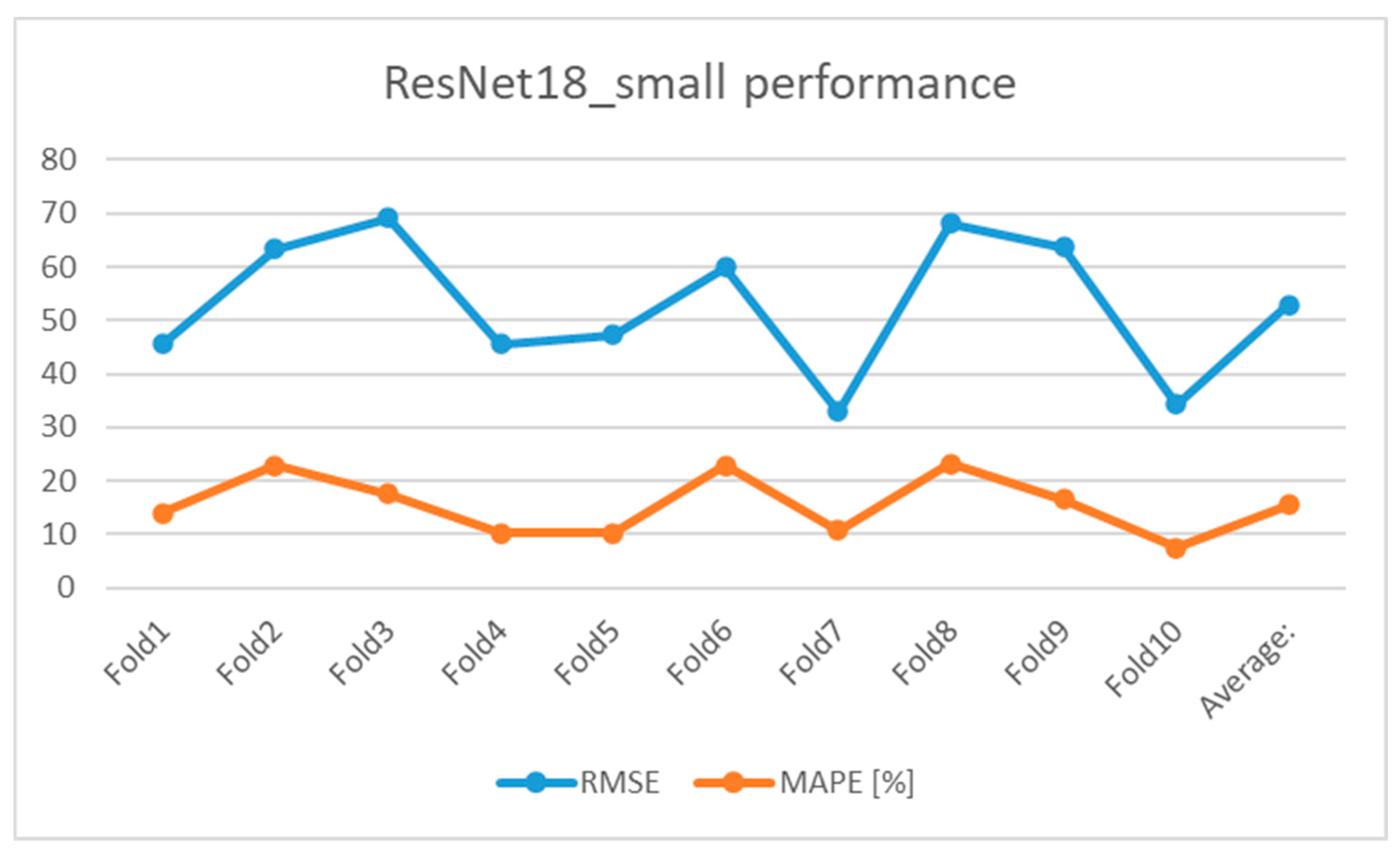
3.1. Statistical Performance of ResNet18_Small

The performance metrics for each fold of the 10-fold CV, including RMSE and MAPE, for ResNet18_small are summarized in

Table 4. ResNet18_small performance metrics.

Fold Number	RMSE [m/min]	MAPE [%]
Fold1	45.58	14.04
Fold2	63.42	22.90
Fold3	69.16	17.58
Fold4	45.62	10.33
Fold5	47.36	10.23
Fold6	59.92	22.93
Fold7	32.96	10.81
Fold8	68.08	23.29
Fold9	63.66	16.49
Fold10	34.36	7.58
Average	53.01	15.62

and Figure 7.

The average RMSE and MAPE across all folds are 53.01 and 15.62%, respectively. The smallest MAPE value was 7.58% in fold 10, while the largest MAPE value was 23.29% in fold 8, resulting in a difference of 15.71 percentage points. Similarly, the smallest RMSE value was 32.96 in fold 7 and the largest RMSE value was 69.16 in fold 3, resulting in a difference of 36.20 units. These differences highlight the small variability in the model’s performance across different folds.

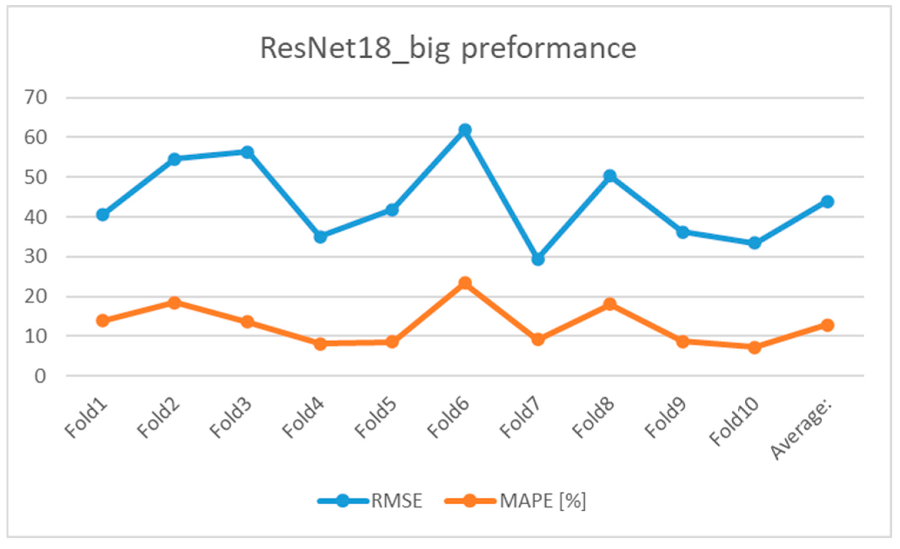
3.2. Statistical Performance of ResNet18_Big

The performance metrics for each fold of the 10-fold CV, including RMSE and MAPE, for ResNet18_big are summarized in

Table 5. ResNet18_big performance metrics.

Fold Number	RMSE [m/mn]	MAPE [%]
Fold1	40.55	13.86
Fold2	54.63	18.39
Fold3	56.33	13.54
Fold4	35.02	8.08
Fold5	41.78	8.58
Fold6	61.76	23.33
Fold7	29.35	9.07
Fold8	50.24	17.93
Fold9	36.26	8.74
Fold10	33.36	7.25
Average	43.93	12.88

and Figure 8.

The average RMSE and MAPE across all folds are 43.93 and 12.88%, respectively. The smallest MAPE value was 7.25% in fold 10, while the largest MAPE value was 23.33% in fold 6, resulting in a difference of 16.08 percentage points. Similarly, the smallest RMSE value was 29.35 in fold 7, and the largest RMSE value was 61.76 in fold 6, resulting in a difference of 32.41 units. These differences highlight the small variability in the model’s performance across different folds.

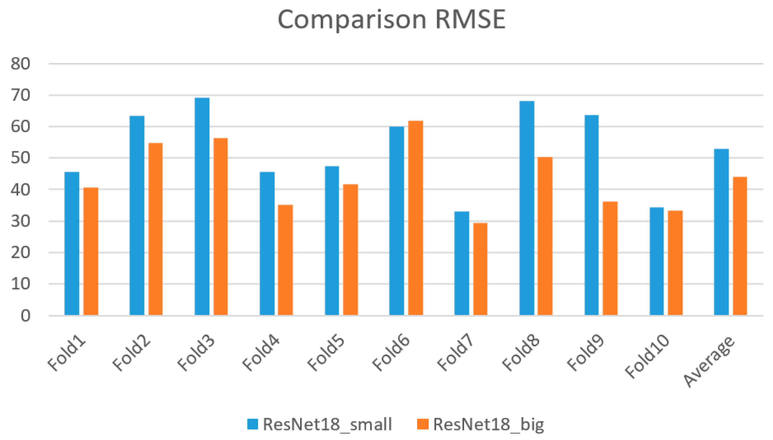
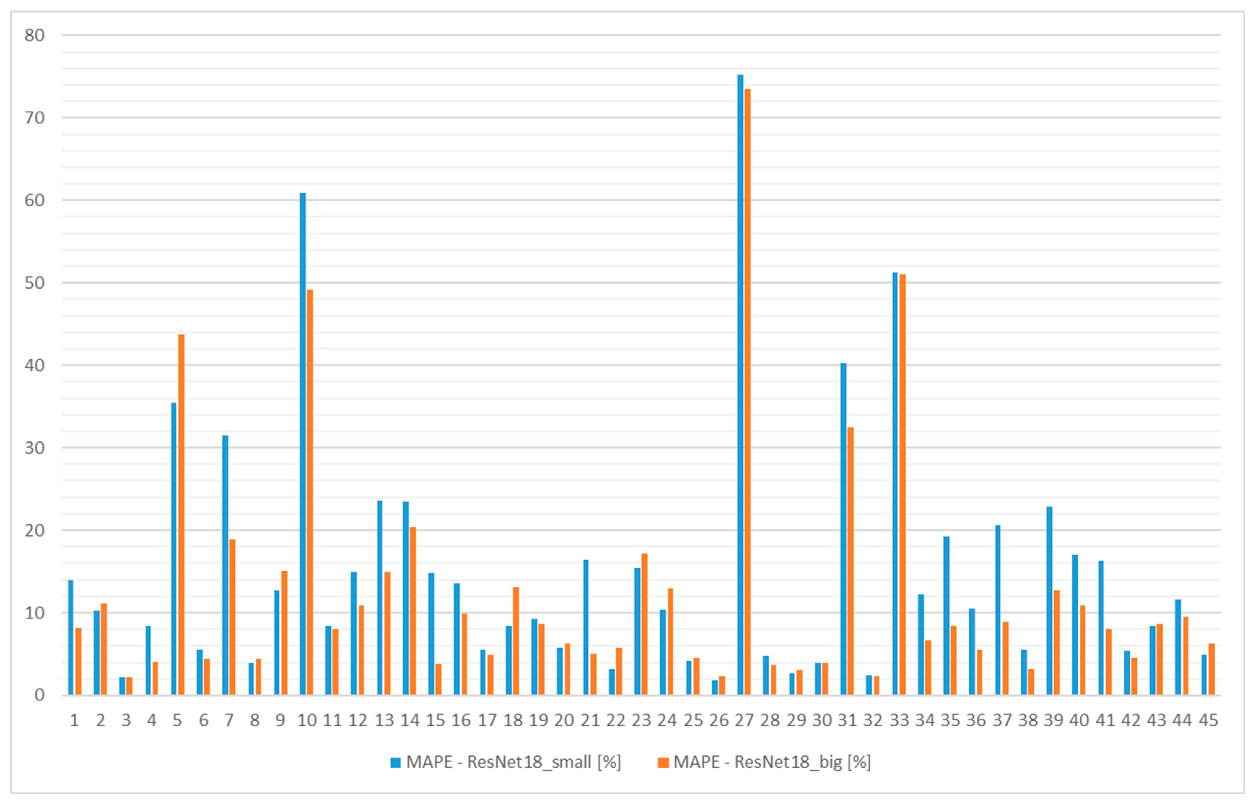
3.3. Comparative Analysis

Figure 9 and Figure 10 provide a visual comparison of the performance between ResNet18_small and ResNet18_big. Figure 9 illustrates the MAPE comparison, while Figure 10 displays the RMSE comparison using bar charts.

The graphs indicate that ResNet18_big consistently achieved lower MAPE and RMSE rates compared to ResNet18_small, confirming the quantitative results. ResNet18_big outperformed ResNet18_small in every fold except for fold 6. This consistent performance across most folds demonstrates the superior capability of ResNet18_big in predicting steel machinability from spark images.

Figure 11 shows the MAPE comparison between the ResNet18 models for each steel sample.

Figure 11 reveals that, while both models predicted some samples with high MAPE errors (30% or higher for five samples), the overall performance for other samples was good, with many samples predicted with MAPE errors less than 5%. This indicates that the models, particularly ResNet18_big, are generally effective in predicting steel machinability despite some outliers. The best machinability predictions using the created model were observed for 16MnCrS5/70/EXEM and 20MnV6/72/EXEM steels, demonstrating the model’s robustness for these specific steel grades. Conversely, the worst predictions were made for 42CrMoS4/70/EXEM and 38MnVS6/70/EXEM steels, indicating potential areas for further model refinement and adjustment to improve accuracy for these materials.

3.4. Observations and Trends

The analysis of the performance metrics revealed several key observations and trends. ResNet18_big demonstrated superior accuracy over ResNet18_small, with consistently lower RMSE and MAPE values across most folds, except for fold 6 where ResNet18_small performed marginally better. This suggests that higher resolution images (700 × 450 pixels) provide more detailed features that are crucial for accurately predicting machinability.

Despite the overall good performance, both models struggled with five specific steel samples, predicting their machinability with MAPE errors of 30% or higher. This indicates potential outliers or complexities in these samples that the models could not accurately capture. On the other hand, a significant number of samples were predicted with MAPE errors of less than 5%, demonstrating the models’ capability to provide highly accurate predictions for the majority of the dataset.

These findings highlight the importance of image resolution in training CNN models for machinability prediction and suggest that further refinement in handling outlier samples could enhance model accuracy. The results also underscore the potential of using spark images for rapid and reliable machinability testing in steel manufacturing.

4. Discussion

In this study, we collected 45 different steel samples with known machinability values obtained from the standard ISO 3685 test [9]. We designed and implemented a grinding experiment and a machine vision system to capture images of sparks produced during the grinding process. The experiments were conducted under controlled conditions using a CNC machine with a ceramic grinding wheel. Enfield electronic pressure regulator was used to ensure a constant cutting force. Spark images were captured during the grinding process and subsequently preprocessed to enhance the quality of the data. We developed CNN models, specifically employing the ResNet18 architecture, to predict the machinability of the steel samples based on these images. The created models were then evaluated using various metrics.

Our study builds on earlier research that employed various machine-learning models to predict machinability. While prior methods relied heavily on physical and chemical properties, our approach uniquely leverages spark image characteristics during grinding. This novel methodology not only aligns with but also advances the current understanding by demonstrating the feasibility of using image-based data for machinability prediction. The error of our method, calculated against the geometrically defined cutting results from the standard ISO 3685 test [9] (where V15 values were assessed), serves as the reference for evaluating the performance of our model. The ability to correlate the V15 values obtained from a standard, well-defined cutting process to those predicted from the non-defined grinding process underscores the practical application of our approach.

Compared to the standard ISO test, which takes several hours to complete, our methodology can detect machinability in a few minutes. This includes preparing the steel sample for grinding, grinding it, capturing images of the sparks, and feeding those images into the CNN model, which then predicts machinability in seconds. The average prediction error was 12.88%. Additionally, our method demonstrated a significant reduction in material usage and required less specialized expertise compared to traditional methods. This approach also has the potential to become fully automatic by integrating the grinding process and machine vision applications into steel plant production, allowing for rapid assessment of the machinability of created steel.

The results from our study demonstrate that ResNet18_big, which uses higher resolution images (700 × 450 pixels), consistently outperforms ResNet18_small, which uses lower resolution images (350 × 225 pixels), in predicting the machinability of steel samples. This finding is in line with previous studies that suggest higher resolution images can provide more detailed features for CNN models, thereby improving prediction accuracy. However, the models’ struggles with certain samples highlight the need for further refinement. These outliers may contain unique features or complexities not well captured by the current models. Addressing these could lead to even more robust predictions.

While our study shows promising results, there are some limitations. The variability in performance across different folds and samples indicates that the models may not yet generalize well to all types of steel samples. Additionally, during predictions, there were some outlier samples with high MAPE values.

Future research should focus on addressing the limitations identified in this study. Enhancing model robustness to handle outlier samples, exploring other image processing techniques, and integrating additional features such as chemical composition or microstructural properties could be beneficial. Moreover, validating the models in real-world manufacturing settings would further solidify the practical applicability of this approach.

In conclusion, our study demonstrates the potential of using CNN models with spark images for the rapid machinability testing of steels. Despite some limitations, the findings offer a promising direction for improving manufacturing efficiency through advanced data-driven methodologies. By effectively correlating the machinability predictions from non-defined cutting (grinding) to those obtained from geometrically defined cutting (ISO 3685 test), this study opens new possibilities for integrating innovative data-mining techniques into traditional manufacturing processes.

References

1. Black, J.T.; Kohser, R.A. DeGarmo’s Materials and Processes in Manufacturing; John Wiley & Sons: Hoboken, NJ, USA, 2017; ISBN 978-1-118-98767-4. [Google Scholar]
2. Davim, J.P. Machinability of Advanced Materials; John Wiley & Sons: Hoboken, NJ, USA, 2014; ISBN 978-1-118-57679-3. [Google Scholar]
3. Maisuradze, M.V.; Björk, T. Microstructure and Mechanical Properties of High-Strength Steel with Improved Machinability. Metallurgist 2022, 66, 391–402. [Google Scholar] [CrossRef]
4. Mills, B.; Redford, A.H. The Assessment of Machinability. In Machinability of Engineering Materials; Mills, B., Redford, A.H., Eds.; Springer: Dordrecht, The Netherlands, 1983; pp. 33–58. ISBN 978-94-009-6631-4. [Google Scholar]
5. Grzesik, W. Advanced Machining Processes of Metallic Materials: Theory, Modelling and Applications; Elsevier: Amsterdam, The Netherlands, 2008; ISBN 978-0-08-055749-6. [Google Scholar]
6. Bellot, J. Steels with Improved Machinability. Met. Sci. Heat Treat. 1980, 22, 794–799. [Google Scholar] [CrossRef]
7. Kovačič, M.; Pšeničnik, M.; Steel, Š.; Slovenia, D. Extra Machinability Modeling Modeliranje Povečane Obdelovalnosti. RMZ–Mater. Geoenviron. 2009, 56, 338–345. [Google Scholar]
8. Alizadeh, E. Factors Influencing the Machinability of Sintered Steels. Powder Metall. Met. Ceram. 2008, 47, 304–315. [Google Scholar] [CrossRef]
9. ISO 3685:1993(En); Tool-Life Testing with Single-Point Turning Tools. ISO: Geneva, Switzerland, 1993. Available online: https://www.iso.org/obp/ui/#iso:std:iso:3685:ed-2:v1:en (accessed on 2 July 2024).
10. ISO 8688-1:1989(En); Tool Life Testing in Milling—Part 1: Face Milling. ISO: Geneva, Switzerland, 1989. Available online: https://www.iso.org/obp/ui/#iso:std:iso:8688:-1:ed-1:v1:en (accessed on 2 July 2024).
11. ISO 8688-2:1989(En); Tool Life Testing in Milling—Part 2: End Milling. ISO: Geneva, Switzerland, 1989. Available online: https://www.iso.org/obp/ui/#iso:std:iso:8688:-2:ed-1:v1:en (accessed on 2 July 2024).
12. Kovačič, M.; Salihu, S.; Gantar, G.; Župerl, U. Modeling and Optimization of Steel Machinability with Genetic Programming: Industrial Study. Metals 2021, 11, 426. [Google Scholar] [CrossRef]
13. Stoić, A.; Kopač, J.; Cukor, G. Testing of Machinability of Mould Steel 40CrMnMo7 Using Genetic Algorithm. J. Mater. Process. Technol. 2005, 164–165, 1624–1630. [Google Scholar] [CrossRef]
14. Boubekri, N.; Rodriguez, J.; Asfour, S. Development of an Aggregate Indicator to Assess the Machinability of Steels. J. Mater. Process. Technol. 2003, 134, 159–165. [Google Scholar] [CrossRef]
15. Šalak, A.; Vasilko, K.; Selecká, M.; Danninger, H. New Short Time Face Turning Method for Testing the Machinability of PM Steels. J. Mater. Process. Technol. 2006, 176, 62–69. [Google Scholar] [CrossRef]
16. Šalak, A.; Selecká, M.; Danninger, H. Machinability of Powder Metallurgy Steels; Cambridge International Science Publishing: Cambridge, UK, 2005; ISBN 978-1-898326-82-3. [Google Scholar]
17. Békés, J. Engineering Technology of Machining of Metals; ALFA: Bratislava, Slovakia, 1981; pp. 89–105. [Google Scholar]
18. Jakubéczyová, D.; Fáberová, M. Mechanical Properties and Surface Treatment PM Cobalt High Speed Steels. Powder Metall. Prog. 2002, 2, 188–197. [Google Scholar]
19. Ebrahimi, A.; Moshksar, M.M. Evaluation of Machinability in Turning of Microalloyed and Quenched-Tempered Steels: Tool Wear, Statistical Analysis, Chip Morphology. J. Mater. Process. Technol. 2009, 209, 910–921. [Google Scholar] [CrossRef]
20. Nomani, J.; Pramanik, A.; Hilditch, T.; Littlefair, G. Machinability Study of First Generation Duplex (2205), Second Generation Duplex (2507) and Austenite Stainless Steel during Drilling Process. Wear 2013, 304, 20–28. [Google Scholar] [CrossRef]
21. Blais, C.; L’Espérance, G.; Bourgeois, I. Characterisation of Machinability of Sintered Steels during Drilling Operations. Powder Metall. 2001, 44, 67–76. [Google Scholar] [CrossRef]
22. Kaladhar, M.; Subbaiah, K.V.; Rao, C.H.S. Machining of Austenitic Stainless Steels—A Review. Int. J. Mach. Mach. Mater. 2012, 12, 178–192. [Google Scholar] [CrossRef]
23. Stephenson, D.A.; Agapiou, J.S. Metal Cutting Theory and Practice, 3rd ed.; CRC Press: Boca Raton, FL, USA, 2018; ISBN 978-1-315-37311-9. [Google Scholar]
24. Ren, L.; Zhang, G.; Wang, Y.; Zhang, Q.; Wang, F.; Huang, Y. A New In-Process Material Removal Rate Monitoring Approach in Abrasive Belt Grinding. Int. J. Adv. Manuf. Technol. 2019, 104, 2715–2726. [Google Scholar] [CrossRef]
25. Wang, N.; Zhang, G.; Ren, L.; Pang, W.; Wang, Y. Vision and Sound Fusion-Based Material Removal Rate Monitoring for Abrasive Belt Grinding Using Improved LightGBM Algorithm. J. Manuf. Process. 2021, 66, 281–292. [Google Scholar] [CrossRef]
26. Ren, L.; Wang, N.; Pang, W.; Li, Y.; Zhang, G. Modeling and Monitoring the Material Removal Rate of Abrasive Belt Grinding Based on Vision Measurement and the Gene Expression Programming (GEP) Algorithm. Int. J. Adv. Manuf. Technol. 2022, 120, 385–401. [Google Scholar] [CrossRef]
27. Rajmohan, B.; Radhakrishnan, V. On the Possibility of Process Monitoring in Grinding by Spark Intensity Measurements. J. Eng. Ind. 1994, 116, 124–129. [Google Scholar] [CrossRef]
28. Deiva Nathan, R.; Vijayaraghavan, L.; Krishnamurthy, R. In-Process Monitoring of Grinding Burn in the Cylindrical Grinding of Steel. J. Mater. Process. Technol. 1999, 91, 37–42. [Google Scholar] [CrossRef]
29. Buzzard, R.W. The Utility of the Spark Test as Applied to Commercial Steels. Bur. Stand. J. Res. 1933, 11, 527. [Google Scholar] [CrossRef]
30. Guillen, A.; Goh, F.; Andre, J.; Barral, A.; Brochet, C.; Louis, Q.; Guillet, T. From the Microstructure of Steels to the Explosion of Sparks. Emergent Sci. 2019, 3, 2. [Google Scholar] [CrossRef]
31. Deng, K.; Pan, D.; Li, X.; Yin, F. Spark Testing to Measure Carbon Content in Carbon Steels Based on Fractal Box Counting. Measurement 2019, 133, 77–80. [Google Scholar] [CrossRef]
32. Pšeničnik, M. Optimizacija Proizvodnje EXEM Jekla v Štore Steel, d.o.o. Master’s Thesis, Univerza v Mariboru, Fakulteta za organizacijske vede, Maribor, Slovenia, 2005. [Google Scholar]
33. LeCun, Y.; Bengio, Y.; Hinton, G. Deep Learning. Nature 2015, 521, 436–444. [Google Scholar] [CrossRef]
34. ImageNet Classification with Deep Convolutional Neural Networks|Communications of the ACM. Available online: https://dl.acm.org/doi/abs/10.1145/3065386 (accessed on 2 July 2024).
35. He, K.; Zhang, X.; Ren, S.; Sun, J. Deep Residual Learning for Image Recognition. arXiv 2016, arXiv:1512.03385. [Google Scholar] [CrossRef]
36. Deep Learning Toolbox. Available online: https://www.mathworks.com/products/deep-learning.html (accessed on 2 July 2024).
37. Weiss, K.; Khoshgoftaar, T.M.; Wang, D. A Survey of Transfer Learning. J. Big Data 2016, 3, 9. [Google Scholar] [CrossRef]
38. Hodson, T.O. Root-Mean-Square Error (RMSE) or Mean Absolute Error (MAE): When to Use Them or Not. Geosci. Model Dev. 2022, 15, 5481–5487. [Google Scholar] [CrossRef]
39. Sutskever, I.; Martens, J.; Dahl, G.; Hinton, G. On the Importance of Initialization and Momentum in Deep Learning. In Proceedings of the 30th International Conference on Machine Learning, Atlanta, GA, USA, 16–21 June 2013; PMLR: New York City, NY, USA, 2013; pp. 1139–1147. [Google Scholar]
40. Kohavi, R. A Study of Cross-Validation and Bootstrap for Accuracy Estimation and Model Selection. Ijcai 2001, 14, 1137–1145. [Google Scholar]
Figure 1. Steel samples.
Metals 14 00955 g001
Figure 2. Experimental setup.
Metals 14 00955 g002
Figure 3. Grinding experiment: (a) start of experiment, (b) start of grinding, (c) end of grinding, and (d) end of experiment, 1 pneumatic cylinder, 2 steel sample, 3 grinding tool, black arrows represent movement and rotation direction of tool, red arrows represent spark direction.
Metals 14 00955 g003
Figure 4. Camera position.
Metals 14 00955 g004
Figure 5. Captured image of sparks.
Metals 14 00955 g005
Figure 6. Image cropping and resizing: (a) original image, (b) cropped image, (c) cropped and resized image 350 × 225 px, and (d) cropped and resized image 700 × 450 px.
Metals 14 00955 g006
Figure 7. ResNet18_small performance.
Metals 14 00955 g007
Figure 8. ResNet18_big performance.
Metals 14 00955 g008
Figure 9. MAPE comparison.
Metals 14 00955 g009
Figure 10. RMSE comparison.
Metals 14 00955 g010
Figure 11. MAPE comparison for each steel sample.
Metals 14 00955 g011