
Design of Point Charge Models for Divalent Metal Cations Targeting Quantum Mechanical Ion–Water Dimer Interactions

Abstract
:1. Introduction
2. Computational Methods
2.1. QM Calculations of Ion–Water Dimers
2.2. LJ Parameter Scanning
2.3. Parameter Generation
2.4. General MD Simulation Setup
2.5. Hydration Free Energy Calculation
2.6. IOD and CN Calculations
2.7. Model Evaluation in Salt Solution
2.8. Model Evaluation in a Metalloprotein
3. Results and Discussion
3.1. Targeted Properties from Gas-Phase QM Calculations
3.2. Designed Model Parameters
3.3. Gas-Phase IE Comparison
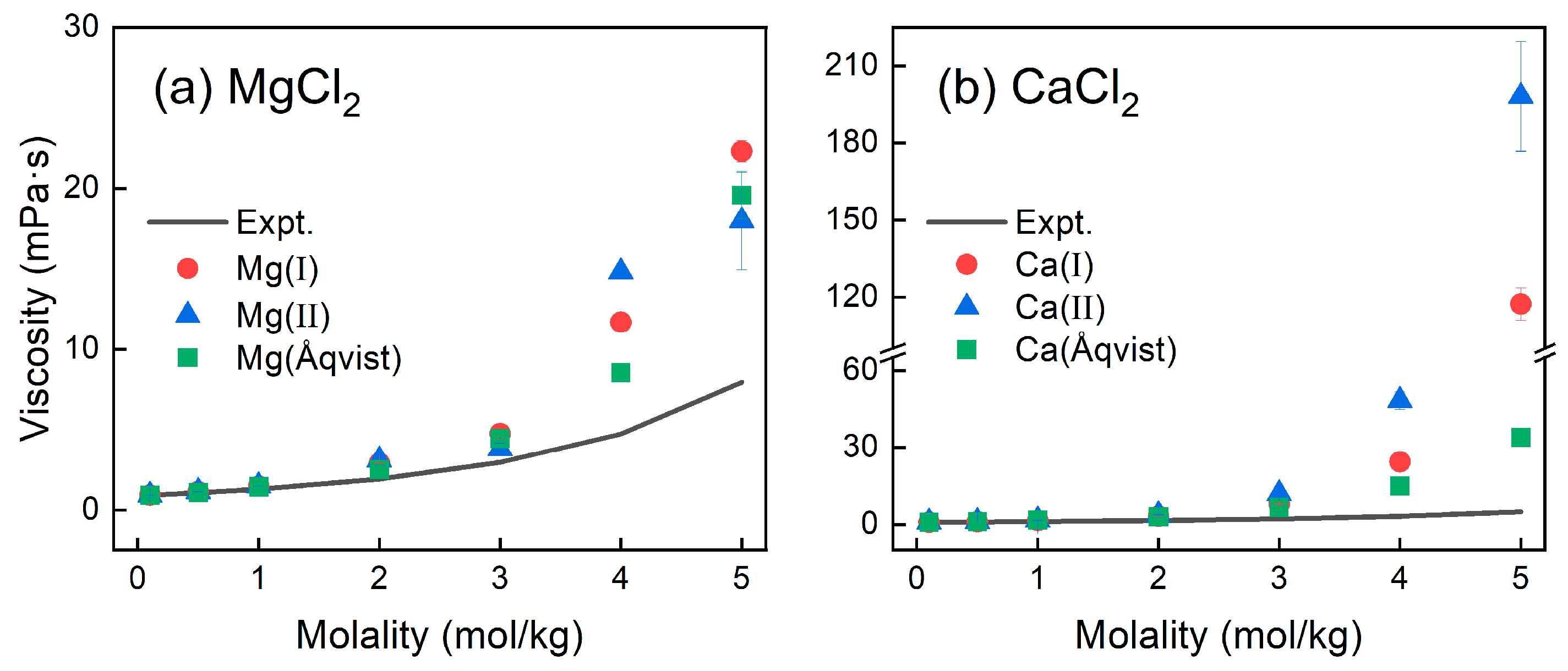
3.4. Density and Viscosity of Salt Solutions
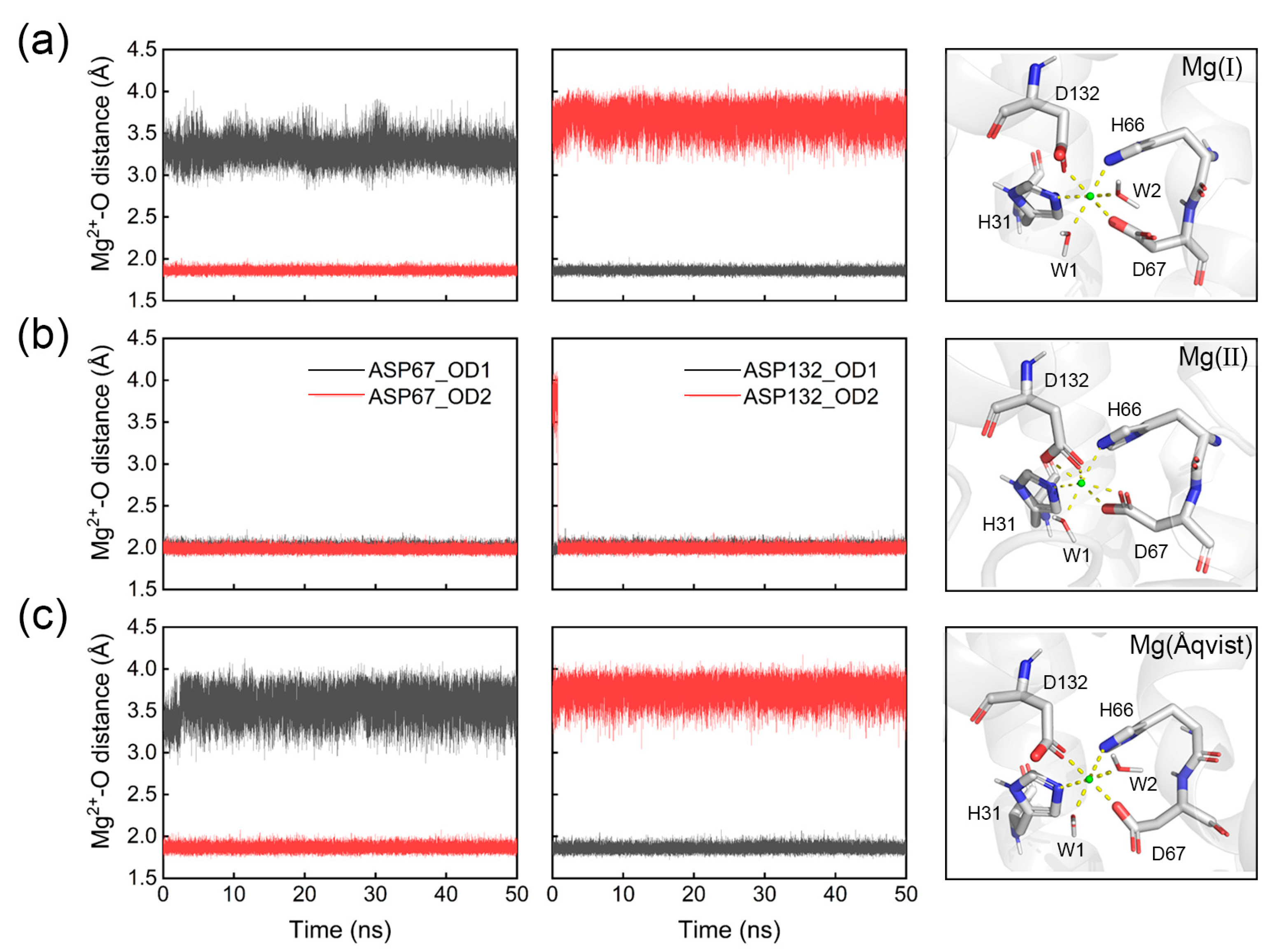
3.5. Metalloprotein Simulation
4. Concluding Remarks
Supplementary Materials
Author Contributions
Funding
Data Availability Statement
Acknowledgments
Conflicts of Interest
References
- Al Alawi, A.M.; Majoni, S.W.; Falhammar, H. Magnesium and Human Health: Perspectives and Research Directions. Int. J. Endocrinol. 2018, 2018, 9041694. [Google Scholar] [CrossRef]
- Berta, D.; Buigues, P.J.; Badaoui, M.; Rosta, E. Cations in Motion: QM/MM Studies of the Dynamic and Electrostatic Roles of H+ and Mg2+ Ions in Enzyme Reactions. Curr. Opin. Struct. Biol. 2020, 61, 198–206. [Google Scholar] [CrossRef] [PubMed]
- Eshra, A.; Schmidt, H.; Eilers, J.; Hallermann, S. Calcium Dependence of Neurotransmitter Release at a High Fidelity Synapse. eLife 2021, 10, e70408. [Google Scholar] [CrossRef]
- Song, Z.; Wang, Y.; Zhang, F.; Yao, F.; Sun, C. Calcium Signaling Pathways: Key Pathways in the Regulation of Obesity. Int. J. Mol. Sci. 2019, 20, 2768. [Google Scholar] [CrossRef] [PubMed]
- Oh, B.-C. Phosphoinositides and Intracellular Calcium Signaling: Novel Insights into Phosphoinositides and Calcium Coupling as Negative Regulators of Cellular Signaling. Exp. Mol. Med. 2023, 55, 1702–1712. [Google Scholar] [CrossRef] [PubMed]
- Rall, J.A. Discovery of the Regulatory Role of Calcium Ion in Muscle Contraction and Relaxation: Setsuro Ebashi and the International Emergence of Japanese Muscle Research. Adv. Physiol. Educ. 2022, 46, 481–490. [Google Scholar] [CrossRef] [PubMed]
- Morrell, A.E.; Brown, G.N.; Robinson, S.T.; Sattler, R.L.; Baik, A.D.; Zhen, G.; Cao, X.; Bonewald, L.F.; Jin, W.; Kam, L.C.; et al. Mechanically Induced Ca2+ Oscillations in Osteocytes Release Extracellular Vesicles and Enhance Bone Formation. Bone Res. 2018, 6, 6. [Google Scholar] [CrossRef]
- Qiao, W.; Pan, D.; Zheng, Y.; Wu, S.; Liu, X.; Chen, Z.; Wan, M.; Feng, S.; Cheung, K.M.C.; Yeung, K.W.K.; et al. Divalent Metal Cations Stimulate Skeleton Interoception for New Bone Formation in Mouse Injury Models. Nat. Commun. 2022, 13, 535. [Google Scholar] [CrossRef]
- Meenachi, P.; Subashini, R.; Lakshminarayanan, A.K.; Gupta, M. Comparative Study of the Biocompatibility and Corrosion Behaviour of Pure Mg,Mg Ni/Ti, and Mg 0.4Ce/ZnO2 Nanocomposites for Orthopaedic Implant Applications. Mater. Res. Express 2023, 10, 056503. [Google Scholar]
- Shan, Z.; Xie, X.; Wu, X.; Zhuang, S.; Zhang, C. Development of Degradable Magnesium-Based Metal Implants and Their Function in Promoting Bone Metabolism (a Review). J. Orthop. Transl. 2022, 36, 184–193. [Google Scholar] [CrossRef]
- Zhao, C.; Tan, J.; Li, W.; Tong, K.; Xu, J.; Sun, D. Ca2+ Ion Responsive Pickering Emulsions Stabilized by Pssma Nanoaggregates. Langmuir 2013, 29, 14421–14428. [Google Scholar] [CrossRef] [PubMed]
- Li, N.; Cao, Y.; Liu, J.; Zou, W.; Chen, M.; Cao, H.; Deng, S.; Liang, J.; Yuan, T.; Wang, Q.; et al. Microenvironment-Responsive Release of Mg2+ from Tannic Acid Decorated and Multilevel Crosslinked Hydrogels Accelerates Infected Wound Healing. J. Mater. Chem. B 2024, 12, 6856–6873. [Google Scholar] [CrossRef]
- Bril, M.; Fredrich, S.; Kurniawan, N.A. Stimuli-Responsive Materials: A Smart Way to Study Dynamic Cell Responses. Smart. Mater. Med. 2022, 3, 257–273. [Google Scholar] [CrossRef]
- Dauber-Osguthorpe, P.; Hagler, A.T. Biomolecular Force Fields: Where Have We Been, Where Are We Now, Where Do We Need to Go and How Do We Get There? J. Comput. Aided Mol. Des. 2019, 33, 133–203. [Google Scholar] [CrossRef] [PubMed]
- Hu, L.H.; Ryde, U. Comparison of Methods to Obtain Force-Field Parameters for Metal Sites. J. Chem. Theory Comput. 2011, 7, 2452–2463. [Google Scholar] [CrossRef]
- Li, P.; Merz, K.M., Jr. Mcpb.Py: A Python Based Metal Center Parameter Builder. J. Chem. Inf. Model. 2016, 56, 599–604. [Google Scholar] [CrossRef] [PubMed]
- Duarte, F.; Bauer, P.; Barrozo, A.; Amrein, B.A.; Purg, M.; Åqvist, J.; Kamerlin, S.C.L. Force Field Independent Metal Parameters Using a Nonbonded Dummy Model. J. Phys. Chem. B 2014, 118, 4351–4362. [Google Scholar] [CrossRef]
- Jiang, Y.; Zhang, H.; Feng, W.; Tan, T. Refined Dummy Atom Model of Mg2+ by Simple Parameter Screening Strategy with Revised Experimental Solvation Free Energy. J. Chem. Inf. Model. 2015, 55, 2575–2586. [Google Scholar] [CrossRef]
- Jiang, Y.; Zhang, H.; Tan, T. Rational Design of Methodology-Independent Metal Parameters Using a Nonbonded Dummy Model. J. Chem. Theory Comput. 2016, 12, 3250–3260. [Google Scholar] [CrossRef]
- Liao, Q.; Pabis, A.; Strodel, B.; Kamerlin, S.C.L. Extending the Nonbonded Cationic Dummy Model to Account for Ion-Induced Dipole Interactions. J. Phys. Chem. Lett. 2017, 8, 5408–5414. [Google Scholar] [CrossRef]
- Peng, J.; Zhang, Y.; Jiang, Y.; Zhang, H. Developing and Assessing Nonbonded Dummy Models of Magnesium Ion with Different Hydration Free Energy References. J. Chem. Inf. Model. 2021, 61, 2981–2997. [Google Scholar] [CrossRef]
- Li, P.; Roberts, B.P.; Chakravorty, D.K.; Merz, K.M., Jr. Rational Design of Particle Mesh Ewald Compatible Lennard-Jones Parameters for +2 Metal Cations in Explicit Solvent. J. Chem. Theory Comput. 2013, 9, 2733–2748. [Google Scholar] [CrossRef]
- Li, P.; Merz, K.M., Jr. Taking into Account the Ion-Induced Dipole Interaction in the Nonbonded Model of Ions. J. Chem. Theory Comput. 2014, 10, 289–297. [Google Scholar] [CrossRef] [PubMed]
- Li, Z.; Song, L.F.; Li, P.; Merz, K.M. Systematic Parametrization of Divalent Metal Ions for the OPC3, OPC, TIP3P-FB, and TIP4P-FB Water Models. J. Chem. Theory Comput. 2020, 16, 4429–4442. [Google Scholar] [CrossRef]
- Zhang, Y.; Jiang, Y.; Peng, J.; Zhang, H. Rational Design of Nonbonded Point Charge Models for Divalent Metal Cations with Lennard-Jones 12-6 Potential. J. Chem. Inf. Model. 2021, 61, 4031–4044. [Google Scholar] [CrossRef] [PubMed]
- Åqvist, J. Ion-Water Interaction Potentials Derived from Free Energy Perturbation Simulations. J. Phys. Chem. 1990, 94, 8021–8024. [Google Scholar] [CrossRef]
- Babu, C.S.; Lim, C. Empirical Force Fields for Biologically Active Divalent Metal Cations in Water. J. Phys. Chem. A 2006, 110, 691–699. [Google Scholar] [CrossRef]
- Allnér, O.; Nilsson, L.; Villa, A. Magnesium Ion-Water Coordination and Exchange in Biomolecular Simulations. J. Chem. Theory Comput. 2012, 8, 1493–1502. [Google Scholar] [CrossRef] [PubMed]
- Man, V.H.; Wu, X.; He, X.; Xie, X.Q.; Brooks, B.R.; Wang, J. Determination of Van Der Waals Parameters Using a Double Exponential Potential for Nonbonded Divalent Metal Cations in TIP3P Solvent. J. Chem. Theory Comput. 2021, 17, 1086–1097. [Google Scholar] [CrossRef]
- Jafari, M.; Li, Z.; Song, L.F.; Sagresti, L.; Brancato, G.; Merz, K.M., Jr. Thermodynamics of Metal–Acetate Interactions. J. Phys. Chem. B 2024, 128, 684–697. [Google Scholar] [CrossRef]
- Li, Z.; Song, L.F.; Sharma, G.; Koca Fındık, B.; Merz, K.M., Jr. Accurate Metal–Imidazole Interactions. J. Chem. Theory Comput. 2023, 19, 619–625. [Google Scholar] [CrossRef] [PubMed]
- Koca Fındık, B.; Jafari, M.; Song, L.F.; Li, Z.; Aviyente, V.; Merz, K.M., Jr. Binding of Phosphate Species to Ca2+ and Mg2+ in Aqueous Solution. J. Chem. Theory Comput. 2024, 20, 4298–4307. [Google Scholar] [CrossRef]
- Nikitin, A.; Del Frate, G. Development of Nonbonded Models for Metal Cations Using the Electronic Continuum Correction. J. Comput. Chem. 2019, 40, 2464–2472. [Google Scholar] [CrossRef]
- Zeron, I.M.; Abascal, J.L.F.; Vega, C. A Force Field of Li+, Na+, K+, Mg2+, Ca2+, Cl−, and SO42− in Aqueous Solution Based on the TIP4P/2005 Water Model and Scaled Charges for the Ions. J. Chem. Phys. 2019, 151, 134504. [Google Scholar] [CrossRef] [PubMed]
- Blazquez, S.; Conde, M.M.; Abascal, J.L.F.; Vega, C. The Madrid-2019 Force Field for Electrolytes in Water Using TIP4P/2005 and Scaled Charges: Extension to the Ions F−, Br−, I−, Rb+, and Cs+. J. Chem. Phys. 2022, 156, 044505. [Google Scholar] [CrossRef] [PubMed]
- Blazquez, S.; Conde, M.M.; Vega, C. Scaled Charges for Ions: An Improvement but Not the Final Word for Modeling Electrolytes in Water. J. Chem. Phys. 2023, 158, 054505. [Google Scholar] [CrossRef]
- Duignan, T.T.; Baer, M.D.; Schenter, G.K.; Mundy, C.J. Real Single Ion Solvation Free Energies with Quantum Mechanical Simulation. Chem. Sci. 2017, 8, 6131–6140. [Google Scholar] [CrossRef]
- Jones, R.O. Density Functional Theory: Its Origins, Rise to Prominence, and Future. Rev. Mod. Phys. 2015, 87, 897–923. [Google Scholar] [CrossRef]
- Verma, P.; Truhlar, D.G. Status and Challenges of Density Functional Theory. Trends Chem. 2020, 2, 302–318. [Google Scholar] [CrossRef]
- Jorgensen, W.L.; Chandrasekhar, J.; Madura, J.D.; Impey, R.W.; Klein, M.L. Comparison of Simple Potential Functions for Simulating Liquid Water. J. Chem. Phys. 1983, 79, 926–935. [Google Scholar] [CrossRef]
- Cornell, W.D.; Cieplak, P.; Bayly, C.I.; Gould, I.R.; Merz, K.M., Jr.; Ferguson, D.M.; Spellmeyer, D.C.; Fox, T.; Caldwell, J.W.; Kollman, P.A. A Second Generation Force Field for the Simulation of Proteins, Nucleic Acids, and Organic Molecules. J. Am. Chem. Soc. 1995, 117, 5179–5197. [Google Scholar] [CrossRef]
- Bridwell-Rabb, J.; Kang, G.; Zhong, A.; Liu, H.-W.; Drennan, C.L. An HD Domain Phosphohydrolase Active Site Tailored for Oxetanocin-a Biosynthesis. Proc. Natl. Acad. Sci. USA 2016, 113, 13750–13755. [Google Scholar] [CrossRef] [PubMed]
- Stephens, P.J.; Devlin, F.J.; Chabalowski, C.F.; Frisch, M.J. Ab Initio Calculation of Vibrational Absorption and Circular Dichroism Spectra Using Density Functional Force Fields. J. Phys. Chem. 1994, 98, 11623–11627. [Google Scholar] [CrossRef]
- Grimme, S.; Ehrlich, S.; Goerigk, L. Effect of the Damping Function in Dispersion Corrected Density Functional Theory. J. Comput. Chem. 2011, 32, 1456–1465. [Google Scholar] [CrossRef]
- Weigend, F.; Ahlrichs, R. Balanced Basis Sets of Split Valence, Triple Zeta Valence and Quadruple Zeta Valence Quality for H to Rn: Design and Assessment of Accuracy. Phys. Chem. Chem. Phys. 2005, 7, 3297–3305. [Google Scholar] [CrossRef]
- Joung, I.S.; Cheatham, T.E., III. Determination of Alkali and Halide Monovalent Ion Parameters for Use in Explicitly Solvated Biomolecular Simulations. J. Phys. Chem. B 2008, 112, 9020–9041. [Google Scholar] [CrossRef]
- Mardirossian, N.; Head-Gordon, M. ωb97x-V: A 10-Parameter, Range-Separated Hybrid, Generalized Gradient Approximation Density Functional with Nonlocal Correlation, Designed by a Survival-of-the-Fittest Strategy. Phys. Chem. Chem. Phys. 2014, 16, 9904–9924. [Google Scholar] [CrossRef]
- Rappoport, D.; Furche, F. Property-Optimized Gaussian Basis Sets for Molecular Response Calculations. J. Chem. Phys. 2010, 133, 134105. [Google Scholar] [CrossRef]
- Mao, Y.; Demerdash, O.; Head-Gordon, M.; Head-Gordon, T. Assessing Ion–Water Interactions in the Amoeba Force Field Using Energy Decomposition Analysis of Electronic Structure Calculations. J. Chem. Theory Comput. 2016, 12, 5422–5437. [Google Scholar] [CrossRef]
- Lu, T.; Chen, F. Multiwfn: A Multifunctional Wavefunction Analyzer. J. Comput. Chem. 2012, 33, 580–592. [Google Scholar] [CrossRef]
- Liu, W.; Hong, G.; Dai, D.; Li, L.; Dolg, M. The Beijing Four-Component Density Functional Program Package (BDF) and Its Application to Euo, Eus, Ybo and Ybs. Theor. Chem. Acc. 1997, 96, 75–83. [Google Scholar] [CrossRef]
- Zhang, Y.; Suo, B.; Wang, Z.; Zhang, N.; Li, Z.; Lei, Y.; Zou, W.; Gao, J.; Peng, D.; Pu, Z.; et al. BDF: A Relativistic Electronic Structure Program Package. J. Chem. Phys. 2020, 152, 064113. [Google Scholar] [CrossRef] [PubMed]
- Liu, W.; Wang, F.; Li, L. The Beijing Density Functional (BDF) Program Package: Methodologies and Applications. J. Theor. Comput. Chem. 2003, 02, 257–272. [Google Scholar] [CrossRef]
- Liu, W.; Wang, F.; Li, L. Relativistic Density Functional Theory: The BDF Program Package. In Recent Advances in Relativistic Molecular Theory; World Scientific Publishing: Singapore, 2004; pp. 257–282. [Google Scholar]
- Abraham, M.J.; Murtola, T.; Schulz, R.; Páll, S.; Smith, J.C.; Hess, B.; Lindahl, E. GROMACS: High Performance Molecular Simulations through Multi-Level Parallelism from Laptops to Supercomputers. SoftwareX 2015, 1, 19–25. [Google Scholar] [CrossRef]
- Darden, T.; York, D.; Pedersen, L. Particle Mesh Ewald: An N.Log(N) Method for Ewald Sums in Large Systems. J. Chem. Phys. 1993, 98, 10089–10092. [Google Scholar] [CrossRef]
- Essmann, U.; Perera, L.; Berkowitz, M.L.; Darden, T.; Lee, H.; Pedersen, L.G. A Smooth Particle Mesh Ewald Method. J. Chem. Phys. 1995, 103, 8577–8593. [Google Scholar] [CrossRef]
- Bussi, G.; Donadio, D.; Parrinello, M. Canonical Sampling through Velocity Rescaling. J. Chem. Phys. 2007, 126, 014101. [Google Scholar] [CrossRef]
- Parrinello, M.; Rahman, A. Polymorphic Transitions in Single Crystals: A New Molecular Dynamics Method. J. Appl. Phys. 1981, 52, 7182–7190. [Google Scholar] [CrossRef]
- Nose, S.; Klein, M.L. Constant Pressure Molecular Dynamics for Molecular Systems. Mol. Phys. 1983, 50, 1055–1076. [Google Scholar] [CrossRef]
- Miyamoto, S.; Kollman, P.A. Settle—An Analytical Version of the Shake and Rattle Algorithm for Rigid Water Models. J. Comput. Chem. 1992, 13, 952–962. [Google Scholar] [CrossRef]
- Hess, B.; Bekker, H.; Berendsen, H.J.C.; Fraaije, J.G.E.M. Lincs: A Linear Constraint Solver for Molecular Simulations. J. Comput. Chem. 1997, 18, 1463–1472. [Google Scholar] [CrossRef]
- Zhang, Y.; Jiang, Y.; Qiu, Y.; Zhang, H. Rational Design of Nonbonded Point Charge Models for Highly Charged Metal Cations with Lennard-Jones 12-6 Potential. J. Chem. Inf. Model. 2021, 61, 4613–4629. [Google Scholar] [CrossRef] [PubMed]
- Qiu, Y.; Jiang, Y.; Zhang, Y.; Zhang, H. Rational Design of Nonbonded Point Charge Models for Monovalent Ions with Lennard-Jones 12-6 Potential. J. Phys. Chem. B 2021, 125, 13502–13518. [Google Scholar] [CrossRef] [PubMed]
- Zhang, J.; Tuguldur, B.; van der Spoel, D. Force Field Benchmark of Organic Liquids. 2. Gibbs Energy of Solvation. J. Chem. Inf. Model. 2015, 55, 1192–1201. [Google Scholar] [CrossRef] [PubMed]
- Misin, M.; Fedorov, M.V.; Palmer, D.S. Hydration Free Energies of Molecular Ions from Theory and Simulation. J. Phys. Chem. B 2016, 120, 975–983. [Google Scholar] [CrossRef] [PubMed]
- Bennett, C.H. Efficient Estimation of Free Energy Differences from Monte Carlo Data. J. Comput. Phys. 1976, 22, 245–268. [Google Scholar] [CrossRef]
- Lamoureux, G.; Roux, B. Absolute Hydration Free Energy Scale for Alkali and Halide Ions Established from Simulations with a Polarizable Force Field. J. Phys. Chem. B 2006, 110, 3308–3322. [Google Scholar] [CrossRef]
- Zhang, H.; Jiang, Y.; Yan, H.; Yin, C.; Tan, T.; van der Spoel, D. Free-Energy Calculations of Ionic Hydration Consistent with the Experimental Hydration Free Energy of the Proton. J. Phys. Chem. Lett. 2017, 8, 2705–2712. [Google Scholar] [CrossRef]
- Zhang, H.; Jiang, Y.; Yan, H.; Cui, Z.; Yin, C. Comparative Assessment of Computational Methods for Free Energy Calculations of Ionic Hydration. J. Chem. Inf. Model. 2017, 57, 2763–2775. [Google Scholar] [CrossRef]
- Zhang, H.; Yin, C.; Jiang, Y.; van der Spoel, D. Force Field Benchmark of Amino Acids: I. Hydration and Diffusion in Different Water Models. J. Chem. Inf. Model. 2018, 58, 1037–1052. [Google Scholar] [CrossRef] [PubMed]
- Song, Y.; Dai, L.L. The Shear Viscosities of Common Water Models by Non-Equilibrium Molecular Dynamics Simulations. Mol. Simulat. 2010, 36, 560–567. [Google Scholar] [CrossRef]
- Maier, J.A.; Martinez, C.; Kasavajhala, K.; Wickstrom, L.; Hauser, K.E.; Simmerling, C. Ff14sb: Improving the Accuracy of Protein Side Chain and Backbone Parameters from Ff99sb. J. Chem. Theory Comput. 2015, 11, 3696–3713. [Google Scholar] [CrossRef] [PubMed]
- Benedict, W.S.; Gailar, N.; Plyler, E.K. Rotation-Vibration Spectra of Deuterated Water Vapor. J. Chem. Phys. 1956, 24, 1139–1165. [Google Scholar] [CrossRef]
- Kim, J.; Lee, H.M.; Suh, S.B.; Majumdar, D.; Kim, K.S. Comparative Ab Initio Study of the Structures, Energetics and Spectra of X−·(H2O)n=1–4 [X=F, Cl, Br, I] Clusters. J. Chem. Phys. 2000, 113, 5259–5272. [Google Scholar] [CrossRef]
- Bajaj, P.; Götz, A.W.; Paesani, F. Toward Chemical Accuracy in the Description of Ion–Water Interactions through Many-Body Representations. I. Halide–Water Dimer Potential Energy Surfaces. J. Chem. Theory Comput. 2016, 12, 2698–2705. [Google Scholar]
- Marcus, Y. Thermodynamics of Solvation of Ions. Part 5.—Gibbs Free Energy of Hydration at 298.15 K. J. Chem. Soc. Faraday Trans. 1991, 87, 2995–2999. [Google Scholar] [CrossRef]
- Hünenberger, P.; Reif, M. Single-Ion Solvation: Experimental and Theoretical Approaches to Elusive Thermodynamic Quantities; Royal Society of Chemistry: Cambridge, UK, 2011. [Google Scholar]
- Gates, J.A.; Wood, R.H. Densities of Aqueous Solutions of Sodium Chloride, Magnesium Chloride, Potassium Chloride, Sodium Bromide, Lithium Chloride, and Calcium Chloride from 0.05 to 5.0 mol kg-1 and 0.1013 to 40 MPa at 298.15 K. J. Chem. Eng. Data 1985, 30, 44–49. [Google Scholar] [CrossRef]
- Laliberté, M.; Cooper, W.E. Model for Calculating the Density of Aqueous Electrolyte Solutions. J. Chem. Eng. Data 2004, 49, 1141–1151. [Google Scholar] [CrossRef]
- Laliberté, M. A Model for Calculating the Heat Capacity of Aqueous Solutions, with Updated Density and Viscosity Data. J. Chem. Eng. Data 2009, 54, 1725–1760. [Google Scholar] [CrossRef]
- Laliberté, M. Model for Calculating the Viscosity of Aqueous Solutions. J. Chem. Eng. Data 2007, 52, 321–335. [Google Scholar] [CrossRef]
- Fan, K.; Zhang, Y.; Qiu, Y.; Zhang, H. Impacts of Targeting Different Hydration Free Energy References on the Development of Ion Potentials. Phys. Chem. Chem. Phys. 2022, 24, 16244–16262. [Google Scholar] [CrossRef] [PubMed]
- Noyes, R.M. Thermodynamics of Ion Hydration as a Measure of Effective Dielectric Properties of Water. J. Am. Chem. Soc. 1962, 84, 513–522. [Google Scholar] [CrossRef]
- Rosseinsky, D.R. Electrode Potentials and Hydration Energies. Theories and Correlations. Chem. Rev. 1965, 65, 467–490. [Google Scholar]
- Fong, K.D.; Sumić, B.; O’Neill, N.; Schran, C.; Grey, C.P.; Michaelides, A. The Interplay of Solvation and Polarization Effects on Ion Pairing in Nanoconfined Electrolytes. Nano Lett. 2024, 24, 5024–5030. [Google Scholar] [CrossRef] [PubMed]
- Park, S.; Park, H.; Park, C.B.; Sung, B.J. The Effects of Polarization on the Rotational Diffusion of Ions in Organic Ionic Plastic Crystals. J. Chem. Phys. 2022, 157, 144501. [Google Scholar] [CrossRef]
- Phan, L.X.; Lynch, C.I.; Crain, J.; Sansom, M.S.P.; Tucker, S.J. Influence of Effective Polarization on Ion and Water Interactions within a Biomimetic Nanopore. Biophys. J. 2022, 121, 2014–2026. [Google Scholar] [CrossRef] [PubMed]
- Zhang, Z.; Zofchak, E.; Krajniak, J.; Ganesan, V. Influence of Polarizability on the Structure, Dynamic Characteristics, and Ion-Transport Mechanisms in Polymeric Ionic Liquids. J. Phys. Chem. B 2022, 126, 2583–2592. [Google Scholar] [CrossRef]
- Lemkul, J.A.; Huang, J.; Roux, B.; MacKerell, A.D., Jr. An Empirical Polarizable Force Field Based on the Classical Drude Oscillator Model: Development History and Recent Applications. Chem. Rev. 2016, 116, 4983–5013. [Google Scholar] [CrossRef]
- Bedrov, D.; Piquemal, J.-P.; Borodin, O.; MacKerell, A.D., Jr.; Roux, B.; Schröder, C. Molecular Dynamics Simulations of Ionic Liquids and Electrolytes Using Polarizable Force Fields. Chem. Rev. 2019, 119, 7940–7995. [Google Scholar] [CrossRef]
- Kognole, A.A.; Aytenfisu, A.H.; MacKerell, A.D. Balanced Polarizable Drude Force Field Parameters for Molecular Anions: Phosphates, Sulfates, Sulfamates, and Oxides. J. Mol. Model. 2020, 26, 152. [Google Scholar] [CrossRef]
- Villa, F.; MacKerell, A.D., Jr.; Roux, B.; Simonson, T. Classical Drude Polarizable Force Field Model for Methyl Phosphate and Its Interactions with Mg2+. J. Phys. Chem. A 2018, 122, 6147–6155. [Google Scholar] [CrossRef] [PubMed]
- Kostal, V.; Jungwirth, P.; Martinez-Seara, H. Nonaqueous Ion Pairing Exemplifies the Case for Including Electronic Polarization in Molecular Dynamics Simulations. J. Phys. Chem. Lett. 2023, 14, 8691–8696. [Google Scholar] [CrossRef] [PubMed]
- Duboué-Dijon, E.; Javanainen, M.; Delcroix, P.; Jungwirth, P.; Martinez-Seara, H. A Practical Guide to Biologically Relevant Molecular Simulations with Charge Scaling for Electronic Polarization. J. Chem. Phys. 2020, 153, 050901. [Google Scholar] [CrossRef] [PubMed]


| Ions | Gas Phase | Liquid Phase | ||||||
|---|---|---|---|---|---|---|---|---|
| Symmetry | IE | IOD | IOD | CN | ||||
| Mg2+ | C2v | −82.14 | 1.92 | 65.5 | −456.0 | 2.090 | 6 | |
| Ca2+ | C2v | −56.67 | 2.23 | 143.1 | −378.4 | 2.460 | 8 | |
| Cl− | C2v | −11.76 | 3.16 | −335.6 | −77.7 | 3.187 | 6–8.5 | |
| Cl− | Cs | −13.76 | 3.12 | −335.6 | −77.7 | 3.187 | 6–8.5 | |
| Ions | Model a | Target Properties b | R (Å) | ε (kcal/mol) | IE (kcal/mol) | IODgas | IODliq | HFE | CN | ||
|---|---|---|---|---|---|---|---|---|---|---|---|
| C2v | Cs | C2v | Cs | ||||||||
| Mg2+ | Mg(I) | IE, IODgas | 0.3293 | 697.6676 | −82.14 | − | 1.93 | − | 1.98 | −539.60 ± 0.53 | 6.0 |
| Mg(II) | IE, IODliq | 0.3927 | 1611.5925 | −81.86 | − | 2.03 | − | 2.09 | −560.57 ± 0.14 | 6.7 | |
| Mg(Åqvist) c | HFE | 0.7926 | 0.8947 | −69.56 | − | 1.89 | − | 1.98 | −457.75 ± 0.17 | 6.0 | |
| Ca2+ | Ca(I) | IE, IODgas | 0.7825 | 69.7699 | −56.67 | − | 2.23 | − | 2.34 | −432.02 ± 0.09 | 8.0 |
| Ca(II) | IE, IODliq | 0.8081 | 445.7715 | −56.95 | − | 2.38 | − | 2.46 | −467.90 ± 0.08 | 9.0 | |
| Ca(Åqvist) c | HFE | 1.7131 | 0.4598 | −38.16 | − | 2.61 | − | 2.70 | −331.98 ± 0.12 | 8.9 | |
| Cl− | Cl(I) | IE, IODgas | 2.3442 | 0.1365 | −13.59 | −13.76 | 3.19 | 3.12 | 3.18 | −77.42 ± 0.07 | 7.7 |
| Cl(II) | IE, IODliq | 2.3021 | 0.1892 | −13.61 | −13.76 | 3.20 | 3.12 | 3.18 | −77.64 ± 0.02 | 7.6 | |
| Cl(JC) d | IE, HFE, LE, LC | 2.5130 | 0.0356 | −13.67 | −13.95 | 3.15 | 3.07 | 3.12 | −76.87 ± 0.07 | 7.3 | |
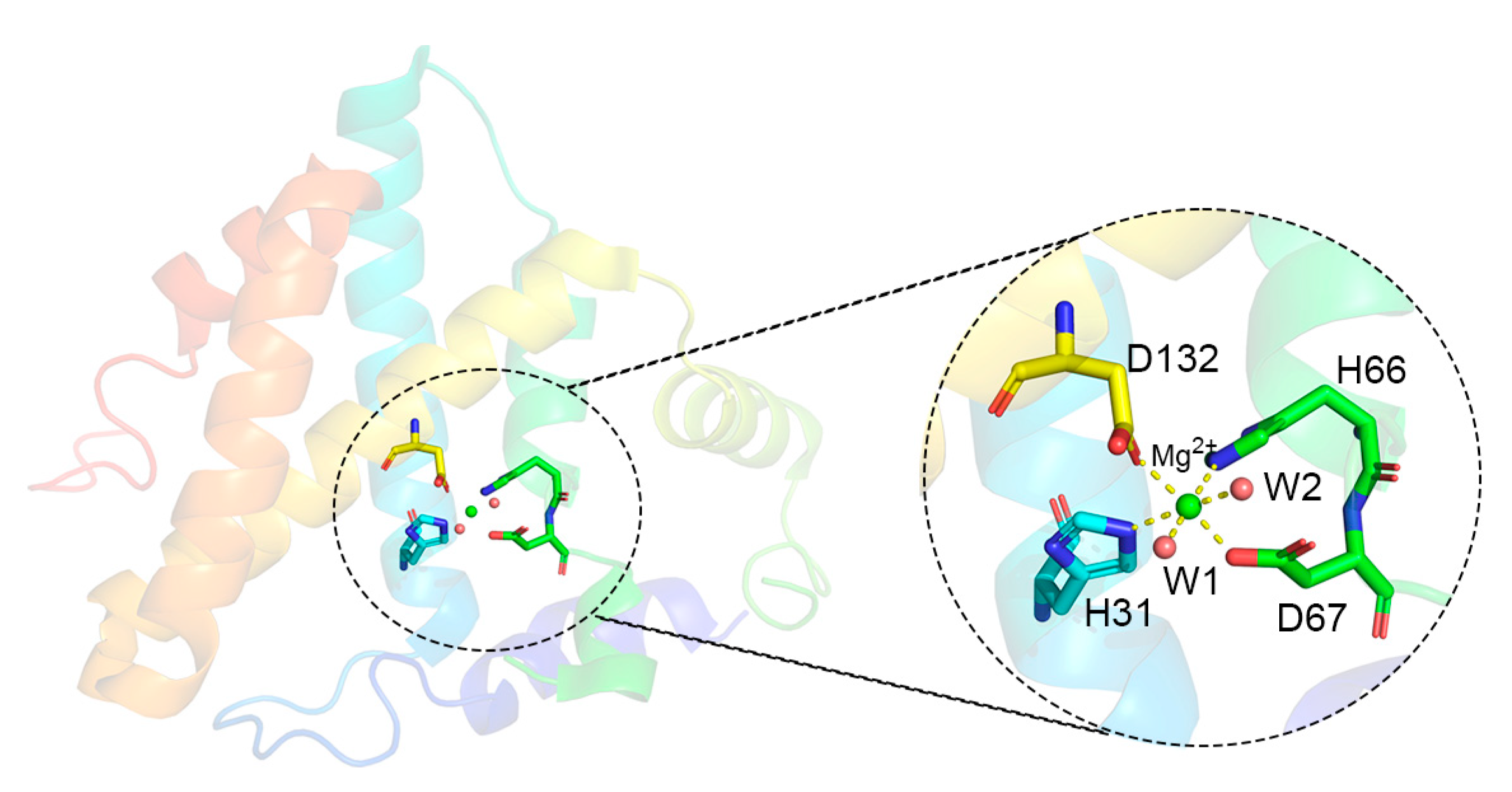
| Model | H31 NE2 | H66 NE2 | D67 OD1 | D67 OD2 | D132 OD1 | D132 OD2 | Water1 | Water2 |
|---|---|---|---|---|---|---|---|---|
| Mg(I) | 2.09 | 2.09 | 3.30 | 1.86 | 1.86 | 3.68 | 2.01 | 2.01 |
| Mg(II) | 2.24 | 2.15 | 2.00 | 1.98 | 2.01 | 1.99 | 2.10 | none |
| Mg(Åqvist) | 2.17 | 2.19 | 3.58 | 1.86 | 1.86 | 3.74 | 2.01 | 2.02 |
| crystal | 2.24 | 2.21 | 3.30 | 2.09 | 2.12 | 3.93 | 1.94 | 1.92 |
Disclaimer/Publisher’s Note: The statements, opinions and data contained in all publications are solely those of the individual author(s) and contributor(s) and not of MDPI and/or the editor(s). MDPI and/or the editor(s) disclaim responsibility for any injury to people or property resulting from any ideas, methods, instructions or products referred to in the content. |
© 2024 by the authors. Licensee MDPI, Basel, Switzerland. This article is an open access article distributed under the terms and conditions of the Creative Commons Attribution (CC BY) license (https://creativecommons.org/licenses/by/4.0/).
Share and Cite
Zhang, Y.; Wu, B.; Lu, C.; Zhang, H. Design of Point Charge Models for Divalent Metal Cations Targeting Quantum Mechanical Ion–Water Dimer Interactions. Metals 2024, 14, 1009. https://doi.org/10.3390/met14091009
Zhang Y, Wu B, Lu C, Zhang H. Design of Point Charge Models for Divalent Metal Cations Targeting Quantum Mechanical Ion–Water Dimer Interactions. Metals. 2024; 14(9):1009. https://doi.org/10.3390/met14091009
Chicago/Turabian StyleZhang, Yongguang, Binghan Wu, Chenyi Lu, and Haiyang Zhang. 2024. "Design of Point Charge Models for Divalent Metal Cations Targeting Quantum Mechanical Ion–Water Dimer Interactions" Metals 14, no. 9: 1009. https://doi.org/10.3390/met14091009