Study of the Thermomechanical Behavior of Single-Crystal and Polycrystal Copper

Abstract

This research paper presents an experimental, theoretical, and numerical study of the thermomechanical behavior of single-crystal and polycrystal copper under uniaxial stress compression loading at varying rates of deformation. The thermomechanical theory is based on a thermodynamically consistent framework for single-crystal face-centered cubic metals, and assumes that all plastic power is partitioned between stored energy due to dislocation structure evolution (configurational) and thermal (kinetic vibrational) energy. An expression for the Taylor–Quinney factor is proposed, which is a simple function of effective temperature and is allowed by second-law restrictions. This single-crystal model is used for the study of single- and polycrystal copper. New polycrystal thermomechanical experimental results are presented at varying strain rates. The temperature evolution on the surface of the polycrystal samples is measured using mounted thermocouples. Thermomechanical numerical single- and polycrystal simulations were performed for all experimental conditions ranging between ${10}^{-3}$ and 5 × ${10}^3$ ${\mathrm{s}}^{-1}$. A Taylor homogenization model is used to represent polycrystal behavior. The numerical simulations of all conditions compare reasonable well with experimental results for both stress and temperature evolution. Given our lack of understanding of the mechanisms responsible for the coupling of dislocation glide and atomic vibration, this implies that the proposed theory is a reasonably accurate approximation of the single-crystal thermomechanics.

1. Introduction

Some of the earliest studies on the conversion of mechanical work to heat in the plastic deformation of metals were by [1,2]. Such energetic considerations are important in the study of the dynamic response of metals in applications such as armor systems and crash testing of vehicles. Study of the thermomechanics of metals has important implications for studying phenomena such as phase transformations [3] and twinning [4], as well as for metal forming and machining. The fraction of the plastic work on a metal that is converted to heat is known as the Taylor–Quinney factor. The complement of this is called the stored energy of cold work.

A common assumption for the fraction of plastic work converted to thermal energy is that it is a constant equal to approximately 0.9, in accordance with the results in [1]. A constant value of 1.0 has also been chosen in the literature [5]. However, experimental results for various pure metals and alloys indicate dependence of the Taylor–Quinney factor on the strain and strain rate. For example, dynamic experiments using the Kolsky bar [6,7] and the dislocation dynamics simulation in [8] indicate that the dislocation accumulation pattern, along with the dislocation density, is important in determining the Taylor–Quinney factor. Study of the thermomechanics of commercially pure titanium reveals that the dissipation of mechanical work as heat may strongly depend on the loading conditions [9]. At high strain rates (≈3000 ${\mathrm{s}}^{-1}$), the authors found that commercially pure titanium shows a profusion of twinning in compression and dominant shear, but not in tension. This corresponds to markedly higher values of the Taylor–Quinney factor for the compression and shear load paths as compared to tension. Quasi-static and dynamic experiments on pure iron [10], polycrystal tantalum [11], single-crystal tantalum [12], and both single-crystal and polycrystal copper [13] provide further experimental evidence of the strain and strain rate dependence of the Taylor–Quinney factor.

The study of crystal mechanics started with work that explicitly embedded the geometry of the slip systems of the material into the kinematical part of the model [14] and by the multiplicative decomposition of the deformation gradient into elastic and plastic parts [15,16,17]. The elastic part of the deformation gradient captures the distortion of the lattice, while the plastic part of deformation gradient captures the transfer of mass along the slip planes of the material. The rotational part of the elastic part of the deformation gradient also contributes to the transfer of mass. The use of such kinematic assumptions has allowed for study of phenomena such as strain localization [18], latent hardening and secondary slip [19,20], and texture evolution [21,22,23], with the combination of these aspects of plastic deformation studied in [24]. Certainly, dislocations behave very differently with crystal atomic structure, which is reflected in the development of continuum crystal mechanics theories [25,26,27,28,29,30,31,32,33,34,35,36,37,38,39,40,41,42,43,44]. Face-centered cubic materials are generally the best understood, with dislocation interaction representing the dominant resistance to motion for most materials. Body-centered cubic materials are very interesting in that the behavior of screw dislocations dominates motion and due to questions about the role of kink–pair nucleation mechanisms in the physics of dislocation motion [45]. Hexagonal close-packed materials differ substantially with material type, as the c/a ratio and corresponding Burgers vector for different slip systems change dramatically [46]. There are many physical factors which impact the thermomechanical response of crystalline materials.

There have also been many important contributions to the development of thermodynamically consistent theories for the description of thermomechanics in crystalline solids, among which are [47,48,49,50,51,52,53,54,55,56,57,58,59,60,61,62,63,64,65,66,67,68,69,70,71,72]. As we develop theories for the description of inelastic processes such as dislocation slip, deformation twinning, structural phase transformation, and damage, accurate partitioning of the energy will provide a stronger physical basis. This forms natural restrictions to our crystal mechanics formulations and provides greater quantitative authority for physical interpretation of experimental results. This naturally affords the need to draw in thermodynamics information from experiments and focused physics calculations. More sophisticated boundary conditions are also necessary in order to document experiments and for application to numerical simulations. Experimental design must then account for the need to characterize thermal boundary conditions and transport properties of materials. Certainly, experiments with higher deformation rate can be assumed to be adiabatic; however, experimental diagnostics are also more limited at higher deformation rates.

This article provides a thermodynamically consistent crystal mechanics framework for solving combined thermomechanical problems in the single and polycrystal mechanics of metallic materials. The fundamental concepts that form the basis of this framework are laid out in [73,74]. On the basis of this theory, a computational framework was developed for polycrystalline isotropic materials and used in [75,76,77]. Further development led to a material model for metal single crystals [78], which is the basis of the computation in this work. The above provides a single-crystal model which captures the strain rate dependence of the thermomechanical behavior. In this model, both the amount of plastic work and the fraction of it converted to heat is dependent on the strain rate. The differential form of the Taylor–Quinney factor is used in this work. The computational model for the polycrystal is a Taylor model, in which the contribution of each individual grain is calculated using the aforementioned single-crystal model. Welded thermocouple beads are used to study the temperature evolution of the sample.

Details of the nomenclature used in this work are provided in

Table 1. Nomenclature table.

Type of Quantity	Description of Symbol	Direct Notation	Indicial Notation
Scalars	Italicized small/cap letters without subscripts or superscripts	a, b, c, A, B, C	a, b, c, A, B, C
Matrices or Vectors	Bold upright letters, using capital letters for vectors in the reference configuration and small letters for vectors in the current configuration.	$\mathbf{u}$, $\mathbf{U}$	$u_i$, $U_i$
Second order tensors	Bold upright letters with underlines, with capital letters for objects in the reference configuration and and small letters for objects in the current configuration.	$\underline{\mathbf{s}}$, $\underline{\mathbf{S}}$	$s_{ij}$, $S_{ij}$
Fourth order tensors	Blackboard bold capital letters.	$\mathbb{C}$	$C_{ijkl}$

. A list of symbols used in the presented theory is provided in

Table 2. List of theory variable symbols.

Variable Symbol	Definition or Meaning
$\underline{\mathbf{F}}$, ${\underline{\mathbf{F}}}^e$, ${\underline{\mathbf{F}}}^p$	Total, elastic, and plastic deformation gradients
$\underline{\mathbf{L}}$, ${\underline{\mathbf{L}}}^e$, ${\underline{\mathbf{L}}}^p$	Total, elastic, and plastic velocity gradients
${\dot{\gamma }}^{\alpha }$	Resolved plastic strain rate on slip system $\alpha$
${\mathbf{s}}^{\alpha }$, ${\mathbf{m}}^{\alpha }$	Unit slip direction vector and normal to slip system $\alpha$
$\underline{\mathbf{T}}$	Cauchy stress tensor
$\underline{\mathbf{S}}$	Second Piola–Kirchhoff stress tensor
$\mathbb{C}$	Anisotropic fourth-order tensor of elastic constants
$C_{11}$, $C_{12}$, $C_{44}$	Independent crystallographic moduli for fcc lattice
$\mu$	Shear modulus
$\mathcal{W}$	Jacobian matrix of stress versus strain
$U_K$, $S_K$	Kinetic–vibrational (thermal) energy and entropy density
$U_C$, $S_C$	Configurational energy and entropy density
$U_D$, $S_D$	Dislocation energy and entropy
$U_1$, $S_1$	Residual configurational energy and entropy density
$F_C$	Configurational free energy density
$e_D$	Dislocation line energy
${\mathbf{q}}_{\mathbf{C}}$, ${\mathbf{q}}_{\mathbf{K}}$	Configurational and thermal fluxes
$\chi$, ${\chi }_0$	Effective temperature and initial effective temperature
$\theta$, T	Thermal temperature (in units of energy and Kelvin)
${\rho }^{\alpha }$	Dislocation density on slip system $\alpha$
${\rho }_{\mathrm{ss}}^{\alpha }$	Steady-state dislocation density on slip system $\alpha$
$v^{\alpha }$	Mean dislocation velocity on slip system $\alpha$
${\chi }_{\mathrm{ss}}$	Steady-state effective temperature (in units of $e_D$)
$\beta$	Taylor–Quinney factor
$c_p$	Specific heat capacity
${\kappa }_{\rho }^{\alpha }$	Dislocation storage rate
${\kappa }_{\chi }$	Effective temperature increase rate
a	Minimum separation between dislocations
b	Burgers vector
$t_0$	Atomic time scale
${\alpha }_T$	Stress scale parameter
${\tau }^{\alpha }$	Resolved shear stress on slip system $\alpha$
$s^{\alpha }$	Slip resistance due to dislocation interaction on slip system $\alpha$
$s_l$	Intrinsic lattice resistance to dislocation motion
${\rho }^{\alpha }$	Dislocation density corresponding to slip system $\alpha$
$l^{\alpha }$	Dislocation mean free path on slip system $\alpha$
$t^{\alpha }$	Dislocation depinning time on slip system $\alpha$
$T_P$	Dislocation depinning barrier (in units of Kelvin)
$a^{\alpha \beta }$	Dislocation interaction tensor
$d^{\alpha \beta }$	Slip interaction tensor
$k_c$, $k_{nc}$	Mean free path parameters

.

2. Materials and Methods

2.1. Theory

This section presents a coupled thermomechanical theory describing the physical behavior of single crystals, which is applied here to face-centered cubic metals and copper in particular.

2.1.1. Plasticity

Based on the theory developed in [15,16,17], it is assumed that the total deformation gradient may be decomposed into elastic and plastic components.

$$\underline{\mathbf{F}}={\underline{\mathbf{F}}}^e{\underline{\mathbf{F}}}^p.$$

(1)

It is assumed that the body starts motion in the reference configuration. It is mapped to the current configuration by the total deformation gradient. The plastic part of the deformation gradient maps the reference configuration to the lattice configuration. The lattice configuration is then mapped to the current configuration by the elastic deformation gradient. The rate of change of plastic deformation in the metal is captured using the plastic velocity gradient, which is a function of the orientations of the all the slip systems and the slip rates on the corresponding slip systems:

$${\underline{\mathbf{L}}}^p={\dot{\underline{\mathbf{F}}}}^p{\left({\underline{\mathbf{F}}}^p\right)}^{-1}=\sum _{\alpha }{\dot{\gamma }}^{\alpha }{\mathbf{s}}^{\alpha }\otimes {\mathbf{m}}^{\alpha },$$

(2)

where ${\mathbf{s}}^{\alpha }$ is a unit vector parallel to the direction of slip on slip system $\alpha$ and ${\mathbf{m}}^{\alpha }$ is a unit vector normal to the slip plane for slip system $\alpha$. The symbol ${\dot{\gamma }}^{\alpha }$ is the rate of slip. The quantities ${\mathbf{s}}^{\alpha }$, ${\mathbf{m}}^{\alpha }$ and ${\underline{\mathbf{L}}}^p$ all inhabit the lattice configuration.

The second Piola–Kirchhoff stress is used as a stress measure in this model, denoted by the symbol $\underline{\mathbf{S}}$ and defined by

$$\underline{\mathbf{S}}=J{\left({\underline{\mathbf{F}}}^e\right)}^{-1}\underline{\mathbf{T}}{\left({\underline{\mathbf{F}}}^e\right)}^{-T},$$

(3)

where $\underline{\mathbf{T}}$ is the Cauchy stress and $J=det\underline{\mathbf{F}}$ is the Jacobian of the total deformation gradient, which is also equal to $det{\underline{\mathbf{F}}}^e$ by the assumption of isochoric plastic deformation. The Cauchy stress inhabits the current configuration, whereas the second Piola–Kirchhoff stress is defined in the lattice configuration.

The stress response is provided by

$$\underline{\mathbf{S}}={\displaystyle \frac{1}{2}}\mathbb{C}:({\left({\underline{\mathbf{F}}}^e\right)}^T{\underline{\mathbf{F}}}^e-\underline{\mathbf{1}})=\mathbb{C}:{\underline{\mathbf{E}}}^e,$$

(4)

where $\mathbb{C}$ and ${\underline{\mathbf{E}}}^e$ are quantities in the lattice configuration, $\mathbb{C}$ is the fourth-order elastic stiffness tensor, and $\underline{\mathbf{1}}$ is the second-order unit tensor. Because copper is a FCC metal, $\mathbb{C}$ has only three independent components. These three elastic moduli describe the behavior of a single crystal that has its <100> directions aligned with the x, y, and z directions of the coordinate axis. The elastic stiffness tensor of a single crystal of any given orientation is calculated by first computing the elasticity tensor of the reference orientation from knowledge of the elastic moduli and then using appropriate tensor transformations to calculate the elasticity tensor for the given orientation. In this work, the temperature dependence of the elastic moduli is accounted for by assuming a linear dependence on temperature as

$$C_{c,ijkl}\left(T\right)=C_{c0,ijkl}+m_{ijkl}T,$$

(5)

where $C_{0,ijkl}$ are the components of the stiffness tensor at 0K and T is the absolute temperature. Of importance to the theory is the resolved shear stress on slip system $\alpha$, denoted by ${\tau }^{\alpha }$ (in the lattice configuration) and provided by

$${\tau }^{\alpha }={\left({\underline{\mathbf{F}}}^e\right)}^T{\underline{\mathbf{F}}}^e\underline{\mathbf{S}}:({\mathbf{s}}^{\alpha }\otimes {\mathbf{m}}^{\alpha })\approx \underline{\mathbf{S}}:({\mathbf{s}}^{\alpha }\otimes {\mathbf{m}}^{\alpha }),$$

(6)

where it is assumed that the elastic deformation in the material is small relative to the plastic deformation. With this assumption, the volume density of plastic power, defined as $\underline{\mathbf{T}}:{\underline{\mathbf{F}}}^e{\underline{\mathbf{L}}}^p{\left({\underline{\mathbf{F}}}^e\right)}^{-1}$, resolves to

$$\begin{array}{c}\hfill \underline{\mathbf{T}}:{\underline{\mathbf{F}}}^e{\underline{\mathbf{L}}}^p{\left({\underline{\mathbf{F}}}^e\right)}^{-1}=\sum _{\alpha }{\tau }^{\alpha }{\dot{\gamma }}^{\alpha }.\end{array}$$

(7)

2.1.2. Thermomechanics

Here, we provide an outline of the crystal mechanics theory. The thermodynamic basis of this work is found in [59,73,74]. After the development of these ideas into isotropic plasticity theories in [75,76,77], a single-crystal version of this theory was presented in [78]. The basic assumption of the theory is that the energy of thermal vibrations is too small to create new dislocations without an applied stress. As a result, it is justifiable to separate the metal into two subsystems: a kinetic–vibrational subsystem, and a configurational subsystem. The latter is characterized by the mean positions of the atoms (and defects) in the metal crystal, while the former is characterized by the motion (vibration) of the atoms about those mean positions. The total volume densities of the system’s energy and entropy are denoted by the symbols $U_{tot}$ and $S_{tot}$, respectively. The assumption described above allows these symbols to be respectively decomposed as $U_{tot}=U_K+U_C$ and $S_{tot}=S_K+S_C$, where the letter K denotes quantities belonging to the kinetic–vibrational subsystem and the letter C denotes quantities belonging to the configurational subsystem. As the configurational subsystem is concerned with the positions of atoms and defects in the lattice, $U_C$ and $S_C$ must depend on the current dislocation density. Denoting the dislocation density on slip system $\alpha$ by ${\rho }^{\alpha }$, we write

$$\begin{array}{cc}\hfill U_C(S_C,{\rho }^{\alpha })& =U_D\left({\rho }^{\alpha }\right)+U_1\left(S_1\right),\hfill \\ \hfill S_C(U_C,{\rho }^{\alpha })& =S_D\left({\rho }^{\alpha }\right)+S_1\left(U_1\right),\hfill \end{array}$$

(8)

where the right-hand sides represent a division of the configurational subsystem into a part dependent on the dislocation population and a part dependent on other sources of imperfection, such as point defects. The following quantity is important in the theory

$$\chi ={\displaystyle \frac{\partial U_C}{\partial S_C}},$$

(9)

where $\chi$ is known as the effective temperature. It characterizes the configurational subsystem by quantifying the atomic disorder in the material relative to a perfect crystal.

In this setup, the local form of the first law of thermodynamics reads $\underline{\mathbf{T}}:\underline{\mathbf{L}}={\dot{U}}_C+{\dot{U}}_K$, where heating contributes to the evolution of $U_K$. Explicitly accounting for heat production and heat fluxes results in

$$\begin{array}{cc}\hfill \underline{\mathbf{T}}:\underline{\mathbf{L}}& ={\dot{U}}_C+{\dot{U}}_K\hfill \\ \hfill & =\chi {\dot{S}}_C+\nabla ·{\mathbf{q}}_C+{\left({\displaystyle \frac{\partial U_C}{\partial t}}\right)}_{S_C,{\rho }^{\alpha }}+\sum _{\alpha }{\left({\displaystyle \frac{\partial U_C}{\partial {\rho }^{\alpha }}}\right)}_{S_C}{\dot{\rho }}^{\alpha }+\theta {\dot{S}}_K+\nabla ·{\mathbf{q}}_K.\hfill \end{array}$$

(10)

Here,

$$\begin{array}{cc}\hfill {\mathbf{q}}_C& =-{\kappa }_C\nabla \chi ,\hfill \\ \hfill {\mathbf{q}}_K& =-\kappa \nabla \theta ,\hfill \end{array}$$

(11)

are the effective and ordinary heat fluxes, respectively, with ${\kappa }_C$ and $\kappa$ as the corresponding conductivities. The symbol $\theta =k_{B}T$ denotes the ordinary temperature in energy units.

The symbol $\underline{\mathbf{L}}$ denotes the velocity gradient, which may be separated into its elastic and plastic components:

$$\underline{\mathbf{L}}={\underline{\mathbf{L}}}^e+{\underline{\mathbf{F}}}^e{\underline{\mathbf{L}}}^p{\underline{\mathbf{F}}}^{e-1}.$$

(12)

With this notation, we write

$${\left({\displaystyle \frac{\partial U_C}{\partial t}}\right)}_{S_C,{\rho }^{\alpha }}=\underline{\mathbf{T}}:{\underline{\mathbf{L}}}^e.$$

(13)

The left-hand side of Equation (13) represents the time rate of change of the internal energy of the system when the configurational state is held constant. By definition, this is the rate of change of the elastic part of the energy. Therefore, the remaining terms on the right-hand side of Equation (10) must add to the plastic power. This is written as

$$\underline{\mathbf{T}}:{\underline{\mathbf{F}}}^e{\underline{\mathbf{L}}}^p{\underline{\mathbf{F}}}^{e-1}=\chi {\dot{S}}_C-{\kappa }_C{\nabla }^2\chi +\sum _{\alpha }{\left({\displaystyle \frac{\partial U_C}{\partial {\rho }^{\alpha }}}\right)}_{S_C}{\dot{\rho }}^{\alpha }+\theta {\dot{S}}_K-\kappa {\nabla }^2\theta .$$

(14)

The second law of thermodynamics in the current context takes the following form

$${\dot{S}}_{\mathrm{tot}}={\dot{S}}_C+{\dot{S}}_K+\nabla ·{\displaystyle \frac{{\mathbf{q}}_C}{\chi }}+\nabla ·{\displaystyle \frac{{\mathbf{q}}_K}{\theta }}\ge 0.$$

(15)

To investigate the consequences of the second law, it is multiplied by $\chi$; quantity $\chi {\dot{S}}_C$ in Equation (15) is eliminated using Equation (14) to obtain the following inequality

$$\begin{array}{cc}\hfill \underline{\mathbf{T}}:{\underline{\mathbf{F}}}^e{\underline{\mathbf{L}}}^p{\underline{\mathbf{F}}}^{e-1}-\sum _{\alpha }{\left({\displaystyle \frac{\partial U_C}{\partial {\rho }^{\alpha }}}\right)}_{S_C}{\dot{\rho }}^{\alpha }& \\ \hfill +(\chi -\theta )\left({\dot{S}}_K-{\displaystyle \frac{\kappa }{\theta }}{\nabla }^2\theta \right)+{\displaystyle \frac{\kappa }{\theta }}{\left(\nabla \theta \right)}^2+{\displaystyle \frac{{\kappa }_c}{\chi }}{\left(\nabla \chi \right)}^2& \ge 0.\hfill \end{array}$$

(16)

The consequences of this inequality can be studied by applying the Coleman–Noll procedure [79]. This procedure allows us to conclude that if a sum of independent terms satisfies an inequality (such as Inequality (16)), each of the terms in the sum must individually satisfy the inequality. Therefore, we write

$$\begin{array}{cc}\hfill \underline{\mathbf{T}}:{\underline{\mathbf{F}}}^e{\underline{\mathbf{L}}}^p{\underline{\mathbf{F}}}^{e-1}& \ge 0,\hfill \\ \hfill -\sum _{\alpha }{\left({\displaystyle \frac{\partial U_C}{\partial {\rho }^{\alpha }}}\right)}_{S_C}{\dot{\rho }}^{\alpha }& \ge 0,\hfill \\ \hfill (\chi -\theta )\left({\dot{S}}_K-{\displaystyle \frac{\kappa }{\theta }}{\nabla }^2\theta \right)& \ge 0,\hfill \\ \hfill {\displaystyle \frac{\kappa }{\theta }}{\left(\nabla \theta \right)}^2& \ge 0,\hfill \\ \hfill {\displaystyle \frac{{\kappa }_c}{\chi }}{\left(\nabla \chi \right)}^2& \ge 0.\hfill \end{array}$$

(17)

The first of these inequalities is guaranteed by Equations (7) and (26). The last two inequalities hold because of the nature of the quantities. The consequences of the third inequality, discussed in detail in [76], are that the Taylor–Quinney factor must be a function of the effective temperature; in addition, as the material approaches a state of maximal disorder, all of the input work turns to thermal energy and the Taylor–Quinney factor must tend to 1.0. Further development of the second inequality shows a derivative of the configurational free energy of the system. Application of the chain rule of calculus to Equations (8) results in

$$\begin{array}{c}\hfill {\left({\displaystyle \frac{\partial U_C}{\partial {\rho }^{\alpha }}}\right)}_{S_C}={\displaystyle \frac{\partial U_D}{\partial {\rho }^{\alpha }}}-{\displaystyle \frac{\partial U_1}{\partial S_1}}{\displaystyle \frac{\partial S_D}{\partial {\rho }^{\alpha }}}.\end{array}$$

(18)

The derivative ${\displaystyle \frac{\partial U_1}{\partial S_1}}$ can be identified as the effective temperature of a part of the configurational subsystem. Because the configurational subsystem has an effective temperature of $\chi$, we have ${\displaystyle \frac{\partial U_1}{\partial S_1}}=\chi$. Therefore, we may write

$$\begin{array}{c}\hfill {\left({\displaystyle \frac{\partial U_C}{\partial {\rho }^{\alpha }}}\right)}_{S_C}={\displaystyle \frac{\partial U_D}{\partial {\rho }^{\alpha }}}-\chi {\displaystyle \frac{\partial S_D}{\partial {\rho }^{\alpha }}}={\displaystyle \frac{\partial (U_D-\chi S_D)}{\partial {\rho }^{\alpha }}}.\end{array}$$

(19)

Here, $F_C\equiv U_D-\chi S_D$ is the configurational free energy. This means that as the dislocation density increases, the free energy tends to minimize and reaches a minimum when ${\dot{\rho }}^{\alpha }=0$. Thus, the steady-state dislocation density minimizes the configurational free energy.

2.1.3. Constitutive Model

Here, we provide details of the computational framework, which was developed in [78] from the theory in [73] described in the previous section. We start from the Orowan relation as

$$\begin{array}{c}\hfill {\dot{\gamma }}^{\alpha }={\rho }^{\alpha }b{v}^{\alpha },\end{array}$$

(20)

where ${\rho }^{\alpha }$ is the mean mobile dislocation density on slip system $\alpha$, b is the magnitude of the Burger’s vector, and $v^{\alpha }$ is the mean dislocation velocity on slip system $\alpha$.

In the physical picture of dislocation motion assumed in this work, the obstacles faced by the dislocation on slip system $\alpha$ have a mean spacing of $l^{\alpha }$. The mean time required by the dislocation to cross this distance is $t^{\alpha }$, meaning that the mean dislocation velocity is $v^{\alpha }=l^{\alpha }/t^{\alpha }$. This expression for the velocity changes the Orowan relation as

$$\begin{array}{c}\hfill {\dot{\gamma }}^{\alpha }={\rho }^{\alpha }b{l}^{\alpha }/t^{\alpha }.\end{array}$$

(21)

This “depinning” of dislocations from obstacles is assumed to be stress-driven and thermally activated. This is accounted for in the expression for the time scale $t^{\alpha }$ as

$$\begin{array}{c}\hfill t^{\alpha }=t_{0}exp\left[{\displaystyle \frac{T_p}{T}}{\left\{1-{\left({\displaystyle \frac{{\tau }^{\alpha }-s_l}{s^{\alpha }}}\right)}^p\right\}}^q\right].\end{array}$$

(22)

Here, $t_0$ is approximately the inverse of the Debye frequency, T is the absolute temperature, and $T_p$ is a measure of the energy barrier to dislocation depinning. The actual energy barrier is provided by $k_B{T}_p$, where $k_B$ is the Boltzmann constant. The symbol ${\tau }^{\alpha }$ denotes the resolved shear stress on slip system $\alpha$, whereas $s_l$ is the intrinsic lattice resistance. The symbol $s^{\alpha }$ denotes the slip resistance due to dislocation interaction on slip system $\alpha$, and is expressed as

$$\begin{array}{c}\hfill s^{\alpha }={\alpha }_T\mu b\sqrt{\sum _{\beta }{a}^{\alpha \beta }{\rho }^{\beta }},\end{array}$$

(23)

where ${\alpha }_T$ is the Taylor factor, accounting for the uncertainty of microstructure and chemical composition of the material. The symbol $\mu$ denotes the shear modulus, which may be calculated from the elastic moduli $C_{11}$, $C_{12}$, and $C_{44}$ using the following expression:

$$\begin{array}{c}\hfill \mu =\sqrt{C_{44}\left({\displaystyle \frac{C_{11}-C_{12}}{2}}\right)}.\end{array}$$

(24)

The symbol $a^{\alpha \beta }$ is a tensor accounting for dislocation interaction. A similar dislocation interaction tensor $d^{\alpha \beta }$ is used to determine the mean free path of the dislocation $l^{\alpha }$:

$$\begin{array}{c}\hfill l^{\alpha }={\displaystyle \frac{1}{\sqrt{{\sum }_{\beta }{d}^{\alpha \beta }{\rho }^{\beta }}}}.\end{array}$$

(25)

The parameters $d^{\alpha \beta }$ are interaction parameters. According to [80], they may be calculated using $a^{\alpha \beta }$, $k_{\mathrm{inter}}$, and $k_{\mathrm{copl}}$, using the expressions $d^{\alpha \beta }={\displaystyle \frac{a^{\alpha \beta }}{k_{\mathrm{inter}}^2}}$ for intersecting slip systems and $d^{\alpha \beta }={\displaystyle \frac{a^{\alpha \beta }}{k_{\mathrm{copl}}^2}}$ for self-interaction and coplanar slip systems. The constants $k_{\mathrm{inter}}$ and $k_{\mathrm{copl}}$ are described in [80], and are related to the inverse proportionality between the mean free path length $l^{\alpha }$ and the resolved shear stress on slip system $\alpha$. Using these expressions, we obtain the following expressions for the slip rate on slip system $\alpha$ as

$$\begin{array}{c}\hfill {\dot{\gamma }}_{|{\tau }^{\alpha }|>0}^{\alpha }={\displaystyle \frac{{\rho }^{\alpha }b}{t_0\sqrt{{\sum }_{\beta }{d}^{\alpha \beta }{\rho }^{\beta }}}}exp\left[-{\displaystyle \frac{T_p}{T}}{\left\{1-{\left({\displaystyle \frac{{\tau }^{\alpha }-s_l}{s^{\alpha }}}\right)}^p\right\}}^q\right]\mathrm{sign}\left({\tau }^{\alpha }\right).\end{array}$$

(26)

Equation (26) is an Arrhenius-type expression. Physically, it corresponds to the idea that dislocations in which atoms have higher kinetic energy (measured by temperature T) have a higher probability of crossing the barrier to dislocation motion (measured by $T_p$). Such flow rules have been used to study localization in polycrystals [81], texture evolution [82], and interface stability in metallic multilayered composites [83] and bicrystals [34]. The effective temperature $\chi$ (with the initial value denoted by ${\chi }_0$) evolves according to

$$\begin{array}{c}\hfill {\displaystyle \frac{\dot{\chi }}{e_D}}={\displaystyle \frac{{\kappa }_{\chi }}{\mu }}\left(1-{\displaystyle \frac{\chi }{{\chi }_{ss}}}\right)\sum _{\beta }{\tau }^{\beta }{\dot{\gamma }}^{\beta },\end{array}$$

(27)

where ${\kappa }_{\chi }$ is a dimensionless parameter. The fraction $\beta ={\displaystyle \frac{\chi }{{\chi }_{ss}}}$ is the Taylor–Quinney factor, and quantifies the fraction of the plastic work that is converted to kinetic vibrational energy. The quantity ${\chi }_{ss}$ is the steady-state effective temperature, which accounts for temperature and strain rate dependence through the following equation:

$$\begin{array}{c}\hfill {\chi }_{ss}={\chi }_{ss0}\left[1+{\displaystyle \frac{1}{N}}\sum _{\alpha }{\left({\displaystyle \frac{|{\dot{\gamma }}^{\alpha }|}{{\dot{\gamma }}_0}}\right)}^{k_{B}T/A}\right]\end{array}$$

(28)

where ${\chi }_{ss0}$ is a material parameter, ${\dot{\gamma }}_0$ is a reference strain rate, A is an activation energy, and N is the number of slip systems ($N=12$ for FCC). The effect of the strain rate is introduced in Equation (28) by raising a strain rate ratio to an exponent of the form $k_{B}T/A$, following similar choices made in [34,81,82,83,84]. The dislocation density (with the initial value denoted by ${\rho }_0$) evolves according to the equation

$$\begin{array}{c}\hfill {\dot{\rho }}^{\alpha }={\displaystyle \frac{{\kappa }_{\rho }^{\alpha }}{a^2}}{\displaystyle \frac{{\tau }^{\alpha }{\dot{\gamma }}^{\alpha }}{\mu }}\left(1-{\displaystyle \frac{{\rho }^{\alpha }}{{\rho }_{ss}^{\alpha }}}\right),\end{array}$$

(29)

where a is a length scale characterizing the critical distance of dislocation interaction and ${\kappa }_{\rho }^{\alpha }$ denotes a parameter for hardening the slip system, calculated according to

$$\begin{array}{c}\hfill {\kappa }_{\rho }^{\alpha }={\displaystyle \frac{{\kappa }_{\rho }^0}{{\nu }_{\alpha }^2}}{\displaystyle \frac{\sqrt{{\rho }_{ss}}-\sqrt{{\rho }^{\alpha }}}{\sqrt{{\rho }_{ss}}-\sqrt{{\rho }_0}}},\end{array}$$

(30)

where ${\kappa }_{\rho }^0$ is a material hardening parameter and ${\rho }_{ss}$ is the steady-state dislocation density, which is calculated from the effective temperature through the equation

$$\begin{array}{c}\hfill {\rho }_{ss}={\displaystyle \frac{1}{a^2}}exp\left(-{\displaystyle \frac{1}{\chi }}\right).\end{array}$$

(31)

Equation (30) introduces a dependence of the hardening behavior of a slip system on the dislocation density of that slip system. The steady-state dislocation density in Equation (31) is also dependent on the deformation rate and temperature through the variable $\chi$. The nominal material hardening is captured by ${\kappa }_{\rho }^0$. At the beginning of deformation, the post-multiplying factor ${\displaystyle \frac{\sqrt{{\rho }_{ss}}-\sqrt{{\rho }^{\alpha }}}{\sqrt{{\rho }_{ss}}-\sqrt{{\rho }_0}}}$ (varying between 0 and 1) equals 1 for all slip systems, as ${\rho }^{\alpha }$ starts with the value ${\rho }_0$ for all slip systems. It decreases as the deformation progresses and dislocation density increases. Therefore, Equation (30) captures the idea that the nature of the material associated with a slip system changes as the dislocation density on that slip system increases. In accordance with [59,60], the parameter ${\nu }_{\alpha }$ is used to calculate ${\kappa }_{\rho }^{\alpha }$ as

$$\begin{array}{c}\hfill {\nu }_{\alpha }=ln\left({\displaystyle \frac{T_p}{T}}\right)-ln\left[ln\left({\displaystyle \frac{b{\rho }^{\alpha }}{t_0\left|\dot{{\gamma }_0^{\alpha }}\right|\sqrt{{\sum }_{\beta }{d}^{\alpha \beta }{\rho }^{\beta }}}}\right)\right],\end{array}$$

(32)

where $\dot{{\gamma }_0^{\alpha }}$ is the total shear rate on slip system $\alpha$.

The temperature then evolves according to the equation

$$\begin{array}{c}\hfill \dot{T}={\displaystyle \frac{1}{\rho C_p}}\left(\beta \sum _{\alpha }{\tau }^{\alpha }{\dot{\gamma }}^{\alpha }+\kappa {\nabla }^2\theta \right),\end{array}$$

(33)

where $\rho$ is the mass density and $C_p$ is the specific heat.

2.2. Computation

All of the simulations were performed using the FEM software ABAQUS/Standard 2023. The material model was specified by writing a UMAT subroutine. The problem domain for all the simulations (single-crystal and polycrystal) was a right circular cylinder. The axis of the cylinder was aligned with the z-axis for the single crystal simulations and aligned with the y-axis for the polycrystal simulations. In both cases, the cylinder was compressed at a constant true strain rate using the ABAQUS user subroutine DISP.

For the single-crystal simulations, the cylinder had a diameter of 6 mm and a height of 6 mm. The crystal was oriented so that the <123> direction of the crystal was initially parallel to the z-axis (the axis along which compression was applied). This was to concentrate most of the slip activity on a single slip plane. Because this asymmetry of sample orientation with respect to the slip systems for copper will not produce an axisymmetric deformation field, full three-dimensional simulations were performed. For single-crystal simulations, the cylinders were compressed at true strain rates of 0.1 ${\mathrm{s}}^{-1}$, 2.0 ${\mathrm{s}}^{-1}$, 3000 ${\mathrm{s}}^{-1}$, and 4800 ${\mathrm{s}}^{-1}$. The element C3D20T from the ABAQUS/Standard element library was chosen to mesh the cylinder domain for the single crystal simulations. These are 20-noded hexahedral thermomechanical elements that use quadratic shape functions. The mesh was comprised of 5120 such elements, and is shown in Figure 1a. This mesh was the smallest element size which would complete a simulation within a reasonable time. The temperature response from the single-crystal simulations was taken as the average of all free surface node temperatures.

For polycrystal simulations, the cylinder had a height of 19.05 mm and diameter of 12.7 mm. The cylinders were compressed at true strain rates of ${10}^{-3}$ ${\mathrm{s}}^{-1}$, ${10}^{-2}$ ${\mathrm{s}}^{-1}$, ${10}^{-1}$ ${\mathrm{s}}^{-1}$, and ${10}^0$ ${\mathrm{s}}^{-1}$. A Taylor model was adopted for the polycrystal simulations. Each element integration point of the Taylor model was assumed to be a composite of 500 randomly oriented grains. All of the grains had distinct randomly distributed orientations, simulating the aggregate response of a random collection of grains at each element integration point. The deformed polycrystal cylindrical samples remained cylindrical during deformation, and there is nothing about the Taylor model representation of the polycrystalline material that would break the axisymmetry. Therefore, an axisymmetric model was used to represent the experiments using two-fold symmetry on both the cylinder axis and length. The behavior of each grain was governed by the same UMAT as that used in the single-crystal simulations.

A half-height axisymmetric model was used for the polycrystal simulations. The left edge of the rectangular mesh shown in Figure 1b is the axis of symmetry. The top edge of the mesh is the axial center of the sample. The mesh was divided into three regions for each of the represented materials (the copper sample, PTFE film lubricant, and tool steel compression platen). The green mesh region of the elements in Figure 1b represents copper. The height of this region was 9.525 mm, with its bottom on the x axis. The width of this region (as well as the other two) was 6.35 mm. The length and diameter of the physical copper samples was 19.05 mm and 12.7 mm, respectively. Just below the copper is a region of elements that is one element in height, representing the lubricating PTFE disk, which is too thin to appear in the figure. The elements in this layer were all 0.0127 mm tall. The remainder of the mesh below the PTFE layer represents the steel compression platens with a height of 9.34 mm (the thickness of the physical steel compression platens). The layer of nodes at the bottom of the copper (top of the PTFE) region was restrained from motion in the y direction, and the user-defined boundary condition was applied to the top of the copper region. Note that the PTFE layer and steel compression platens were included in the polycrystal simulation model for only the thermal transport part of the problem. Neither material played a role in the mechanical part of the problem. Only the copper region of the numerical model contributed to the calculation of the copper stress–strain curves.

A Taylor polycrystal model was used to represent the polycrystal copper material. The element CAX8T was used to mesh the rectangular area shown in Figure 1b, with 100 elements representing both the copper and steel and 10 elements representing the PTFE film. Doubling the number of elements did not lead to any noticeable difference in results. These are axisymmetric and thermomechanical eight-node elements with quadratic shape functions. The mesh consisted of 200 such elements. Every integration point in the model was assumed to be a composite of 500 randomly-oriented grains. At every integration point, the function encoding the material model for the single crystal was called 500 times with the same deformation gradient but different grain orientations. The output of these 500 function calls was averaged and returned to ABAQUS as the output of the computation at the integration point. Because the presence of both PTFE and steel in the polycrystal simulations was for heat transport only, both were modeled as isotropic elastic materials with extremely low stiffness, ensuring that they could expand freely with the copper cylinder. Realistic thermal properties were used to represent both materials. Both the copper/PTFE and PTFE/steel interface surfaces defined by connecting nodes were forced to remain fixed in the y-direction.

Following mechanical deformation with the thermomechanical mesh shown in Figure 1b, the cooling transient was simulated using a heat transfer model of the deformed sample shown in Figure 1c. The DCAX8 element was used for this problem, which was initialized for temperature at each node from the results of the thermomechanical problem for the appropriate strain rate condition. This enabled evaluation of the thermal transport film coefficient for the outer surface of the model to represent the thermal transport transient measured experimentally for each condition. Note that the simulated temperature for both the thermomechanical and heat transfer analyses was taken as the position of the thermocouple, which is the node in the top right-hand corner of each of the two axisymmetric meshes.

2.2.1. Mechanical Tangent Operators

To calculate nodal forces and displacements with a user-defined constitutive model at the end of time step $n+1$, ABAQUS/Standard requires the the user to estimate the Cauchy stress ($\underline{\mathbf{T}}$) and Jacobian matrix of the constitutive model ${\mathbb{W}}_{EP}={\displaystyle \frac{\partial \underline{\mathbf{T}}}{\partial \underline{\mathbf{e}}}}$. These quantities are calculated using information from time step n, which is supplied to the user by ABAQUS. In the following, a quantity with a subscript n refers to a quantity calculated in the previous resolved time step, while subscript $n+1$ refers to a quantity involved in the current unresolved time step calculation. The relative deformation gradient ${\underline{\mathbf{F}}}_{\mathrm{rel}}$ is defined as ${\underline{\mathbf{F}}}_{n+1}={\underline{\mathbf{F}}}_{\mathrm{rel}}{\underline{\mathbf{F}}}_n$. The symbol $\underline{\mathbf{e}}=ln\underline{\mathbf{U}}$, where $\underline{\mathbf{U}}$ is the relative stretch portion of the polar decomposition of the relative deformation gradient. By ABAQUS convention, $\underline{\mathbf{T}}$ and $\underline{\mathbf{e}}$ are both defined as $6\times 1$ column vectors with the following forms:

$$\underline{\mathbf{T}}=\left[\begin{array}{c}{T}_{11,n+1}\\ T_{22,n+1}\\ T_{33,n+1}\\ T_{12,n+1}\\ T_{13,n+1}\\ T_{23,n+1}\end{array}\right],\underline{\mathbf{e}}=\left[\begin{array}{c}{e}_{11,n+1}\\ e_{22,n+1}\\ e_{33,n+1}\\ e_{12,n+1}\\ e_{13,n+1}\\ e_{23,n+1}\end{array}\right].$$

Here, we show the method of deriving the fourth-rank tensor ${\mathbb{W}}_{EP}={\displaystyle \frac{\partial \underline{\mathbf{T}}}{\partial \underline{\mathbf{e}}}}$. The $6\times 6$ matrix required by ABAQUS can then be calculated using the following formula:

$$W_{EP}=\left[\begin{array}{cccccc}{W}_{1111}& W_{1122}& W_{1133}& (W_{1112}+W_{1121})/2& (W_{1113}+W_{1131})/2& (W_{1123}+W_{1132})/2\\ W_{2211}& W_{2222}& W_{2233}& (W_{2212}+W_{2221})/2& (W_{2213}+W_{2231})/2& (W_{2223}+W_{2232})/2\\ W_{3311}& W_{3322}& W_{3333}& (W_{3312}+W_{3321})/2& (W_{3313}+W_{3331})/2& (W_{3323}+W_{3332})/2\\ W_{1211}& W_{1222}& W_{1233}& (W_{1212}+W_{1221})/2& (W_{1213}+W_{1231})/2& (W_{1223}+W_{1232})/2\\ W_{1311}& W_{1322}& W_{1333}& (W_{1312}+W_{1321})/2& (W_{1313}+W_{1331})/2& (W_{1323}+W_{1332})/2\\ W_{2311}& W_{2322}& W_{2333}& (W_{2312}+W_{2321})/2& (W_{2313}+W_{2331})/2& (W_{2323}+W_{2332})/2\end{array}\right].$$

(34)

We follow the Jacobian derivation method provided in [85]. We make the assumption that the incremental stretch is small, which is justified because the time steps taken by ABAQUS are reasonably small. This allows us to make the following mathematical simplification: $\underline{\mathbf{e}}=ln\underline{\mathbf{U}}\approx \underline{\mathbf{U}}-1\Rightarrow \delta \underline{\mathbf{e}}=\delta \underline{\mathbf{U}}$. To derive the material Jacobian, we note that the Cauchy stress can be written in terms of the second Piola–Kirchhoff stress $\underline{\mathbf{S}}$:

$$\begin{array}{c}\hfill {\underline{\mathbf{T}}}_{n+1}={\displaystyle \frac{1}{det{\underline{\mathbf{F}}}_{n+1}^e}}\left[{\underline{\mathbf{F}}}_{n+1}^e{\underline{\mathbf{S}}}_{n+1}^e{\underline{\mathbf{F}}}_{n+1}^{eT}\right].\end{array}$$

Taking a derivative of this expression with respect to $\underline{\mathit{e}}$ and introducing the tensors $\mathbb{X}={\displaystyle \frac{\partial {\underline{\mathbf{F}}}^e}{\partial \underline{\mathbf{e}}}}$ and $\mathbb{Q}={\displaystyle \frac{\partial \underline{\mathbf{S}}}{\partial \underline{\mathbf{e}}}}$, we obtain the following equation:

$$\begin{array}{c}\hfill W_{ijkl}={\displaystyle \frac{1}{det{\underline{\mathbf{F}}}^e}}\left[X_{imkl}{S}_{mn}{F}_{nj}^{eT}+F_{im}^e{Q}_{mnkl}{F}_{nj}^{eT}+F_{im}^e{S}_{mn}{X}_{jnkl}-F_{im}^e{S}_{mn}{F}_{nj}^{eT}\left(X_{pqkl}{F}_{qp}^{e-1}\right)\right].\end{array}$$

(35)

Using the small stretch assumption made above, we write $\mathbb{X}\approx {\displaystyle \frac{\partial {\underline{\mathbf{F}}}^e}{\partial \underline{\mathbf{U}}}}$ and $\mathbb{Q}\approx {\displaystyle \frac{\partial \underline{\mathbf{S}}}{\partial \underline{\mathbf{U}}}}$. The following steps, taken from [85], are used to compute the tangent modulus ${\mathbb{W}}_{EP}$. This symbol is written in blackboard bold font to emphasize that it is a fourth-order tensor and that its components are to be used to construct the actual 6 × 6 matrix (using Equation (34)) that is passed back to ABAQUS.

• Compute the fourth-rank tensor $\mathbb{L}$:

  $$\begin{array}{c}\hfill L_{ijkl}=F_{ik,n}^{eT}{U}_{lm,n+1}{F}_{mj,n}^e+F_{im,n}^{eT}{U}_{mk,n+1}{F}_{ij,n}^e.\end{array}$$

  (36)
• Compute the elastic stiffness tensor (${\mathbb{C}}_c$ denotes the elastic stiffness tensor in the crystal frame). To calculate the elastic stiffness tensor for the current grain orientation, the rotation tensor from the reference orientation to the current orientation is denoted by $\underline{\mathbf{Q}}$, and is used to calculate the elastic stiffness tensor using the expression $C_{ijkl}=Q_{ip}{Q}_{jq}{Q}_{kr}{Q}_{ls}{C}_{c,pqrs}$.
• Use the quantities from steps 1 and 2 to calculate the fourth-rank tensor $\mathbb{D}$:

  $$\begin{array}{c}\hfill D_{ijkl}={\displaystyle \frac{1}{2}}{C}_{ijmn}{L}_{mnkl}.\end{array}$$

  (37)
• For each slip system $\alpha$, use the Schmid tensor ${\mathbf{S}}^{\alpha }={\mathbf{s}}^{\alpha }\otimes {\mathbf{m}}^{\alpha }$ to compute the fourth-rank tensors ${\mathbb{G}}^{\alpha }$ and ${\mathbb{J}}^{\alpha }$ and the second-rank tensor ${\underline{\mathbf{B}}}^{\alpha }$:

  $$\begin{array}{cc}\hfill G_{mnkl}^{\alpha }& =L_{mpkl}{S}_{pn}^{\alpha }+L_{pnkl}{S}_{pm}^{\alpha },\hfill \end{array}$$

  (38)

  $$\begin{array}{cc}\hfill J_{ijkl}^{\alpha }& ={\displaystyle \frac{1}{2}}{C}_{ijmn}{G}_{mnkl}^{\alpha },\hfill \end{array}$$

  (39)

  $$\begin{array}{cc}\hfill B_{ij}^{\alpha }& ={\displaystyle \frac{1}{2}}\Delta t{\displaystyle \frac{\partial {\dot{\gamma }}_n^{\alpha }}{\partial {\tau }^{\alpha }}}\left(S_{ij}^{\alpha }+S_{ji}^{\alpha }\right).\hfill \end{array}$$

  (40)
• Compute the fourth-rank tensors $\mathbb{K}$ and $\mathbb{Q}$, which requires summing over all slip systems:

  $$\begin{array}{cc}\hfill K_{ijkl}& =I_{ijkl}+\sum _{\alpha }{C}_{ij}^{\alpha }{B}_{kl}^{\alpha },\hfill \end{array}$$

  (41)

  $$\begin{array}{cc}\hfill Q_{ijkl}& =K_{ijmn}^{-1}\left(D_{mnkl}-\sum _{\alpha }\dot{\gamma }\Delta t{J}_{mnkl}^{\alpha }\right).\hfill \end{array}$$

  (42)
• Compute the following quantities:

  $$\begin{array}{cc}\hfill R_{ij}^{\alpha }& =B_{kl}^{\alpha }{Q}_{klij},\hfill \\ \hfill X_{ijkl}& =R_{ik}\left(F_{lj}^e\left(t_n\right)-F_{lp}^e\left(t_n\right)\sum _{\alpha }{\dot{\gamma }}^{\alpha }\Delta t{S}_{pj}^{\alpha }\right)-R_{im}{U}_{mn}{F}_{np}^e\left(t_n\right)\sum _{\alpha }{R}_{kl}^{\alpha }{S}_{pj}^{\alpha }.\hfill \end{array}$$

  (43)
  The $R_{ik}$ appearing in the computation of $\mathbb{X}$ represents the rotation components of the relative deformation gradient.
• As the final step, compute the Jacobian for the mechanical behavior of the material:

  $$W_{ijkl}={\displaystyle \frac{1}{det{\underline{\mathbf{F}}}^e}}\left[X_{imkl}{S}_{mn}{F}_{jn}^e+F_{im}^e{Q}_{mnkl}{F}_{jn}^e+F_{im}^e{S}_{mn}{X}_{jnkl}-F_{im}^e{S}_{mn}{F}_{jn}^e\left(X_{pqkl}{F}_{qp}^{e-1}\right)\right].$$

  (44)

2.2.2. Thermal Tangent Operators

ABAQUS/Standard forms the tangent matrix for the thermal transport problem using certain quantities provided by the user. The calculation methodology for these quantities is shown in this section. Several derivatives are important in these calculations. The first of these is the variation of ${\dot{\gamma }}^{\alpha }$ with respect to ${\tau }^{\alpha }$:

$$\begin{array}{cc}\hfill {\displaystyle \frac{\partial {\dot{\gamma }}^{\alpha }}{\partial {\tau }^{\alpha }}}=& {\displaystyle \frac{pq{\rho }^{\alpha }{l}^{\alpha }b{T}_p}{s^{\alpha }{t}_{0}T}}exp\left[-{\displaystyle \frac{T_p}{T}}{\left(1-{\left({\displaystyle \frac{{\tau }^{\alpha }-s_l}{s^{\alpha }}}\right)}^p\right)}^q\right]\times \hfill \\ \hfill & \left[{\left(1-{\left({\displaystyle \frac{{\tau }^{\alpha }-s_l}{s^{\alpha }}}\right)}^p\right)}^{q-1}\right]\left[{\left({\displaystyle \frac{{\tau }^{\alpha }-s_l}{s^{\alpha }}}\right)}^{p-1}\right].\hfill \end{array}$$

(45)

The above must be multiplied by the sign of ${\tau }^{\alpha }$. The derivative of ${\dot{\gamma }}^{\alpha }$ with respect to the temperature is provided by

$$\begin{array}{cc}\hfill {\displaystyle \frac{\partial {\dot{\gamma }}^{\alpha }}{\partial T}}=& {\displaystyle \frac{{\rho }^{\alpha }{l}^{\alpha }b}{t_0}}{\displaystyle \frac{T_p}{T^2}}exp\left[-{\displaystyle \frac{T_p}{T}}{\left(1-{\left({\displaystyle \frac{{\tau }^{\alpha }-s_l}{s^{\alpha }}}\right)}^p\right)}^q\right]\times \hfill \\ & \left[{\left(1-{\left({\displaystyle \frac{{\tau }^{\alpha }-s_l}{s^{\alpha }}}\right)}^p\right)}^q\right].\hfill \end{array}$$

(46)

Using these derivatives we can calculate the following four quantities, which are required by ABAQUS for calculating the tangent operators connected to the thermal part of the thermomechanical problem:

• $r_{pl}$: The portion of the mechanical work done on the material that is transformed to heat. It is calculated here as a portion of the plastic work done on the material. It is calculated as $\beta {\sum }_{\alpha }{\tau }^{\alpha }{\dot{\gamma }}^{\alpha }$, where $\beta$ is the Taylor–Quinney factor, $\alpha$ denotes the index for one of 12 slip systems in the metal, ${\tau }^{\alpha }$ is the resolved shear stress on slip system $\alpha$, and ${\dot{\gamma }}^{\alpha }$ is the slip rate on the same slip system.
• The variation of the Cauchy stress with respect to temperature: In this work, we assume that the thermal variation of the Cauchy stress arises from the thermal variation of the elastic moduli of the single crystal. This expression is derived from the definition of the second Piola–Kirchhoff stress:

  $$\begin{array}{cc}\hfill {\displaystyle \frac{\partial \underline{\mathbf{T}}}{\partial T}}& ={\displaystyle \frac{1}{det{\underline{\mathbf{F}}}^e}}{\underline{\mathbf{F}}}^e{\displaystyle \frac{\partial \underline{\mathbf{S}}}{\partial T}}{\underline{\mathbf{F}}}^{eT},\hfill \end{array}$$

  (47)

  $$\begin{array}{cc}\hfill {\displaystyle \frac{\partial S_{ij}}{\partial T}}& =Q_{ip}{Q}_{jq}{Q}_{ks}{Q}_{lr}{m}_{pqrs}{E}_{kl}^e.\hfill \end{array}$$

  (48)
  The temperature dependence of the elastic moduli, and consequently of the Cauchy stress, is obtained from Equation (5).
• The variation of $r_{pl}$ with respect to temperature:

  $$\begin{array}{cc}\hfill r_{pl}& =\beta \sum _{\alpha }{\tau }^{\alpha }{\dot{\gamma }}^{\alpha }\hfill \\ \hfill {\displaystyle \frac{\partial r_{pl}}{\partial T}}& =\beta \sum _{\alpha }\left[{\displaystyle \frac{\partial {\tau }^{\alpha }}{\partial T}}{\dot{\gamma }}^{\alpha }+{\tau }^{\alpha }{\displaystyle \frac{\partial {\dot{\gamma }}^{\alpha }}{\partial T}}\right],\hfill \end{array}$$

  (49)

  $$\begin{array}{cc}\hfill {\displaystyle \frac{\partial {\tau }^{\alpha }}{\partial T}}& ={\displaystyle \frac{\partial \underline{\mathbf{S}}}{\partial T}}:({\mathbf{s}}^{\alpha }\otimes {\mathbf{m}}^{\alpha }).\hfill \end{array}$$

  (50)
• The variation of $r_{pl}$ with respect to the strain:

  $$\begin{array}{cc}\hfill {\displaystyle \frac{\partial r_{pl}}{\partial E_{ij}}}& \approx {\displaystyle \frac{\partial r_{pl}}{\partial U_{ij}}}\hfill \\ \hfill & =\beta \sum _{\alpha }\left[{\displaystyle \frac{\partial {\tau }^{\alpha }}{\partial U_{ij}}}{\dot{\gamma }}^{\alpha }+{\tau }^{\alpha }{\displaystyle \frac{\partial {\dot{\gamma }}^{\alpha }}{\partial U_{ij}}}\right],\hfill \end{array}$$

  (51)

  $$\begin{array}{cc}\hfill {\displaystyle \frac{\partial {\tau }^{\alpha }}{\partial U_{ij}}}& ={\displaystyle \frac{\partial \underline{\mathbf{S}}}{\partial U_{ij}}}:({\mathbf{s}}^{\alpha }\otimes {\mathbf{m}}^{\alpha }).\hfill \end{array}$$

  (52)
  The derivatives of $\underline{\mathbf{S}}$ and ${\dot{\gamma }}^{\alpha }$ with respect to $\underline{\mathbf{U}}$ are denoted by the symbols $\mathbb{Q}$ and $\underline{\mathbf{J}}$, respectively, and appear in the derivation of the mechanical Jacobian.

2.2.3. Mechanical and Thermal Quantities for the Taylor Polycrystal Model

The quantities described in Section 2.2.1 and Section 2.2.2 are those calculated for describing the behavior of single crystals. For the Taylor polycrystal, these quantities are calculated for each of 500 grain orientations assigned to each integration point of the Taylor model aggregate. Each of the 500 calculations assumes the deformation gradient assigned to the integration point by ABAQUS. From the UMAT of the Taylor model, the mean of these 500 quantities is returned to the ABAQUS global equation solver:

• Cauchy stress.
• Tangent stiffness moduli in Equation (34).
• Rate of thermal energy generated.
• Derivative of the Cauchy stress with respect to the temperature.
• Derivative of the rate of thermal energy generation with respect to the temperature.
• Derivative of the rate of thermal energy generation with respect to the strain.

2.3. Experiment

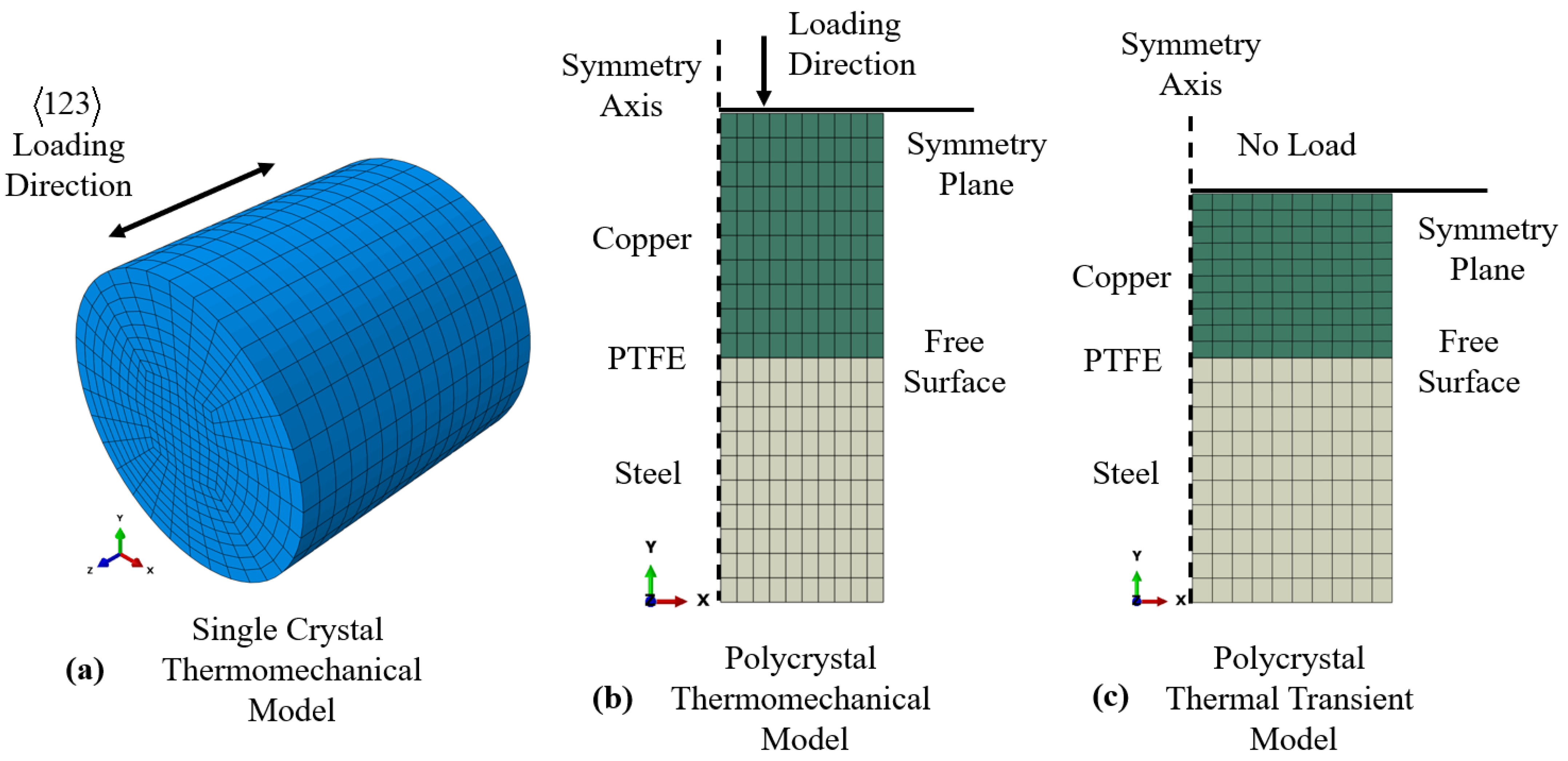
2.3.1. Single-Crystal Experiments

Stress–strain and temperature evolution data were respectively taken from Figures 2b and 5a of [13] for comparison to the single-crystal simulations.

The samples in these experiments were copper right-circular cylinders with diameter 6 mm and height 4–6 mm. They were machined from stock cylinders which had the <123> direction of the single crystal oriented parallel to the axis of the cylinder. The reason for this alignment was to concentrate the plastic slip, at least at the onset of plastic flow, onto a single slip system.

The single-crystal samples were then compressed in the quasi-static regime using an MTS system (Eden Prairie, MN, USA) under displacement control and in the dynamic regime using Kolsky bars of diameter 12.7 mm made of C300 maraging steel. For the quasi-static regime, the temperature of the sample was measured by recording thermal images of the sample as it was being compressed using a thermal imaging camera. For the dynamic regime, thermal detection was carried out using a liquid nitrogen-cooled MCT (mercury–cadmium–telluride) detector. This detector measures temperatures over an area of 100 μm × 100 μm.

To minimize issues related to surface roughness and surface oxidation, the samples were thermally conditioned by preheating to 200 °C for 1 min to ensure that all samples had similar surface conditions.

2.3.2. Polycrystal Experiments

The polycrystal experiments consisted of uniaxial stress compression tests in which the stress, strain, and temperature evolution of the sample were measured simultaneously. Temperature measurements were taken using thermocouples (J type) welded to the outside center of the sample. The samples were right-circular cylinders machined from half-inch round bar stock of OFHC polycrystalline copper. The slenderness ratio of all the samples was equal to or less than 1.5. As such, the lengths of the samples were less than or equal to 0.75 inches (19.05 mm) and their diameters were 0.5 inches (12.7 mm). After machining, the samples were annealed in an Argon-flushed furnace by holding the samples at 800 °C for 1 h and allowing the samples to cool naturally in the same furnace. Thermocouple beads were welded onto the annealed samples using a thermocouple spot welder. Displacement of the sample height reduction was measured using an MTS extensometer mounted directly to the radial surface of cylindrical high-strength steel compression platens 6 inches in diameter and 2 inches thick. These experiments were conducted using a high-capacity Instron servo-hydraulic test system with displacement control on the extensometer to impose a constant true strain rate on the sample for the duration of the experiment. The flat ends of the sample were lubricated for the duration of the compression test by inserting circular pieces of PTFE film of thickness 0.0127 mm and diameter 0.5 inches (the same as the samples).

2.4. Material Parameter Evaluation

The starting point for material parameter evaluation was the list provided in Table 2 of [78]. However, the provided material parameters cannot be used as-is, since the current model differs from [78] in Equations (22) and (28). The list of material parameters used here is provided in

Table 3. List of material parameters for single-crystal simulations. For the polycrystal simulations, all values are the same except for those quantities in parentheses. The symbol ${\rho }_0$ denotes the initial dislocation density on each slip system.

Material Parameter Symbol	Value
$\rho$	8960 Kg/m3
$C_p$	380 J/Kg-K
$K_T$	394 W/m-K
$C_{11,0}$	179,500 MPa
$C_{12,0}$	126,400 MPa
$C_{44,0}$	82,500 MPa
$m_{11}$	$-36.3$ MPa/K
$m_{12}$	$-16.4$ MPa/K
$m_{44}$	$-25.7$ MPa/K
${\alpha }_T$	$2.75$$\left(2.0\right)$
b	$2.57\times {10}^{-7}$ mm
${\rho }_0$	$1\times {10}^5$ mm−2 ($2\times {10}^5$ mm−2)
${\chi }_0$	$0.20$$\left(0.19\right)$
${\chi }_{ss,0}$	$0.25$$\left(0.115\right)$
${\mathrm{a}}_{\mathrm{self}}$	$0.122$
${\mathrm{a}}_{\mathrm{copl}}$	$0.122$
${\mathrm{a}}_{\mathrm{hirth}}$	$0.070$
${\mathrm{a}}_{\mathrm{colli}}$	$0.625$
${\mathrm{a}}_{\mathrm{gliss}}$	$0.137$
${\mathrm{a}}_{\mathrm{lomer}}$	$0.122$
$e_D$	$1.0$
$t_0$	$1\times {10}^{-12}$ s
$T_p$	40,800 K
$k_B$	$1.38\times {10}^{-23}$ J/K
a	$10b$
${\kappa }_{\rho }^0$	60 $\left(68\right)$
${\kappa }_{\chi }$	$3.3$$\left(4.3\right)$
${\dot{\gamma }}_0$	${10}^5$ ${\mathrm{s}}^{-1}$
$k_{\mathrm{copl}}$	15
$k_{\mathrm{inter}}$	200
A	$17.1\times {10}^{-19}$ J
$s_l$	0 MPa
p	$0.33$
q	$1.66$

. All parameters are used for both single- and polycrystal calculation except where different polycrystal values are provided in parentheses. The elastic constants $C_{11,0}$, $C_{12,0}$, and $C_{44,0}$ characterize FCC Copper at 0 K. As mentioned in describing Equation (5), it is assumed that the elastic moduli decrease linearly with the temperature. These variation parameters are $m_{11}$, $m_{12}$, and $m_{44}$. These elastic moduli and their temperature variation parameters were estimated from [86]. For a given temperature T, the three elastic moduli are provided by

$$\begin{array}{cc}\hfill C_{11}\left(T\right)& =C_{11,0}+m_{11}T,\hfill \\ \hfill C_{12}\left(T\right)& =C_{12,0}+m_{12}T,\hfill \\ \hfill C_{44}\left(T\right)& =C_{44,0}+m_{44}T.\hfill \end{array}$$

(53)

Using these elastic constants, the elastic stiffness tensor at a temperature T of the single-crystal orientation used as reference is

$$\begin{array}{cc}\hfill C_{c,ijkl}& =C_{11}\left(T\right)\mathrm{if}i=j=k=l,\hfill \\ \hfill \mathrm{otherwise},C_{c,ijkl}& =C_{12}\left(T\right){\delta }_{ij}{\delta }_{kl}+C_{44}\left(T\right)({\delta }_{ik}{\delta }_{jl}+{\delta }_{il}{\delta }_{kj}).\hfill \end{array}$$

(54)

The values of the matrix entries $a^{\alpha \beta }$ used in Equation (23) depend on relative orientations of the slip normals and slip directions of the slip system corresponding to $\alpha$ and $\beta$:

• $a^{\alpha \alpha }=a_{\mathrm{self}}$: Captures the interaction of a dislocation with other dislocations in the same slip system.
• $a^{\alpha \beta }=a_{\mathrm{copl}}$, if ${\mathbf{m}}^{\alpha }={\mathbf{m}}^{\beta }$ and ${\mathbf{s}}^{\alpha }\ne {\mathbf{s}}^{\beta }$: This corresponds to the dislocation interactions that lead to the formation of dipoles.
• $a^{\alpha \beta }=a_{\mathrm{hirth}}$, if ${\mathbf{m}}^{\alpha }\ne {\mathbf{m}}^{\beta }$ and ${\mathbf{s}}^{\alpha }\perp {\mathbf{s}}^{\beta }$: This corresponds to the formation of a Hirth lock.
• $a^{\alpha \beta }=a_{\mathrm{colli}}$, if ${\mathbf{m}}^{\alpha }\ne {\mathbf{m}}^{\beta }$ and ${\mathbf{s}}^{\alpha }={\mathbf{s}}^{\beta }$: This corresponds to collinear interactions between dislocations.
• $a^{\alpha \beta }=a_{\mathrm{gliss}}$, if ${\mathbf{m}}^{\alpha }\ne {\mathbf{m}}^{\beta }$ and ${\mathbf{s}}^{\alpha }\ne {\mathbf{s}}^{\beta }$: This corresponds to the formation of a glissile junction.
• $a^{\alpha \beta }=a_{\mathrm{lomer}}$ for other configurations of slip normals and slip directions: Corresponds to the formation of a Lomer lock.

The values $a_{\mathrm{self}}$, $a_{\mathrm{copl}}$, $a_{\mathrm{hirth}}$, $a_{\mathrm{colli}}$, $a_{\mathrm{gliss}}$, and $a_{\mathrm{lomer}}$ were calculated from the DD (Dislocation Dynamics) simulations in [37,87,88]. According to [80], the parameters $d^{\alpha \beta }$ needed in Equation (25) can be calculated using $a^{\alpha \beta }$, $k_{\mathrm{inter}}$ and $k_{\mathrm{copl}}$, using the expressions $d^{\alpha \beta }={\displaystyle \frac{a^{\alpha \beta }}{k_{\mathrm{inter}}^2}}$ for intersecting slip systems and $d^{\alpha \beta }={\displaystyle \frac{a^{\alpha \beta }}{k_{\mathrm{copl}}^2}}$ for self-interaction and coplanar slip systems. The same approach is followed in the present work.

The material parameter A introduced in this work is an energy barrier term, and controls the temperature and rate sensitivity of ${\chi }_{ss}$. Because the slip rate on any slip system is usually less than the reference slip rate ${\dot{\gamma }}_0$, a lower value of A corresponds to a higher value of ${\chi }_{ss}$. Because $\chi$ is a measure of the disorder of the system, a higher value of ${\chi }_{ss}$ corresponds to a higher value of the saturation stress of the material. Therefore, a lower value of A corresponds to a strong material. The symbol ${\chi }_0$ denotes the initial value of $\chi$.

Saturation flow stress increases with strain rate [81,84]. The state variable $\chi$ is a measure of the configurational disorder in the system. Therefore, its saturation value ${\chi }_{ss}$ should decrease with temperature. From [84], it is apparent that saturation flow stress decreases as temperature increases. For a FCC material, the saturation flow stress is strongly controlled by the saturation dislocation density. The dislocation content is a measure of the configurational disorder of a system. Therefore, based on experimental data on the saturation value of flow stress, we can make inferences about the saturation value of the configurational disorder of the system. This notion is captured by Equation (28) for variation of ${\chi }_{ss}$.

Several of the material parameters in this work are different from the material parameters in [78] such as ${\kappa }_{\chi }$, ${\kappa }_{\rho }^0$, $k_{\mathrm{copl}}$, $k_{\mathrm{inter}}$, and ${\alpha }_T$. Differences in the first two quantities are related to differences in the effective temperature and dislocation evolution equations. The remaining three may be related to manufacturing differences in the materials being simulated.

Both PTFE and tool steel were used in the polycrystal simulations and represented for thermal transport characteristics only. For PTFE, $\rho =2200$ Kg/m³, $K_T=0.25$ W/m-K, and $C_p=1500$ J/Kg-K; For steel, $\rho =7850$ Kg/m³, $K_T=45$ W/m-K, and $C_p=420$ J/Kg-K.

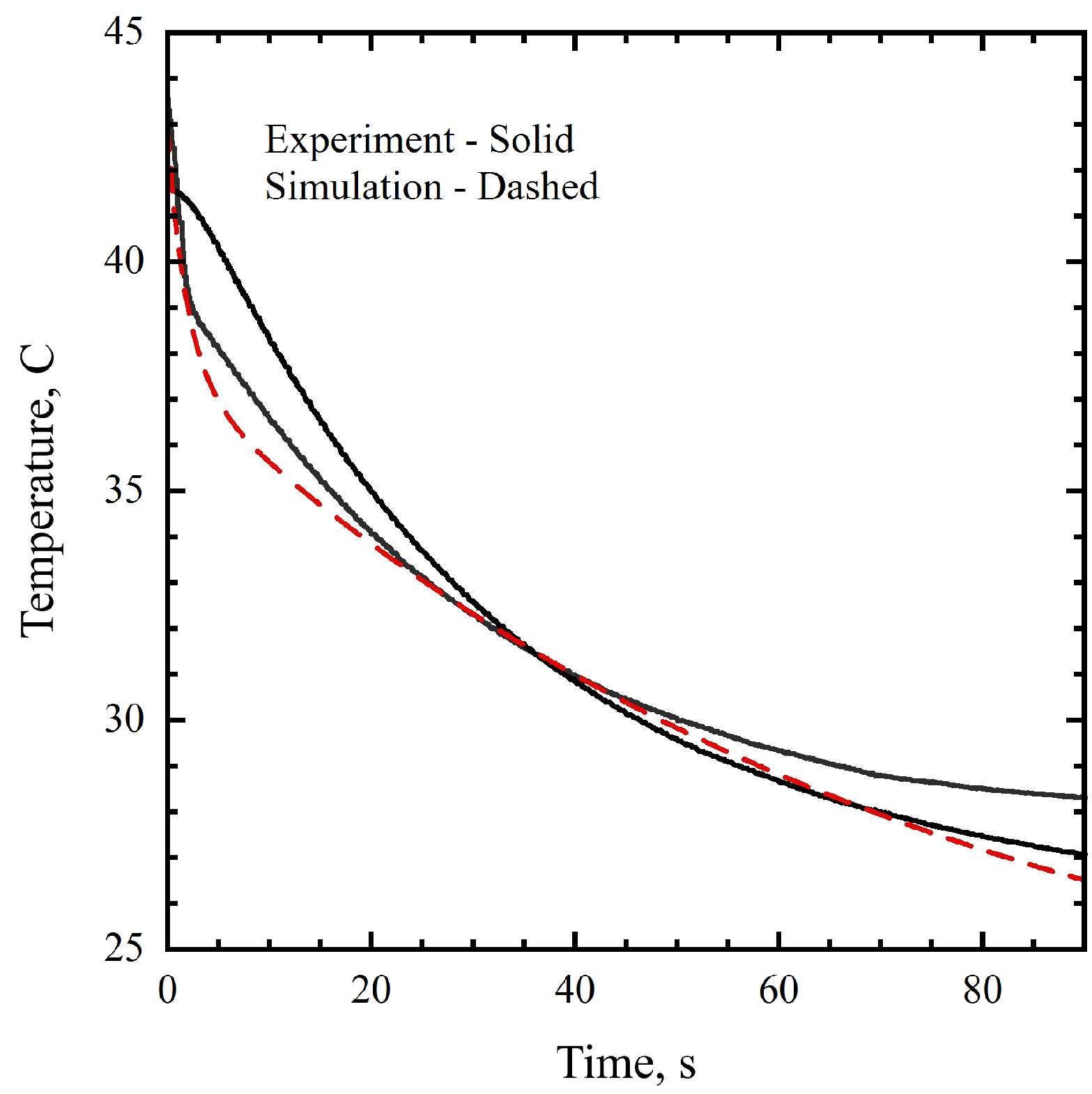
2.5. Free Surface Heat Transfer Coefficient Parameter Evaluation

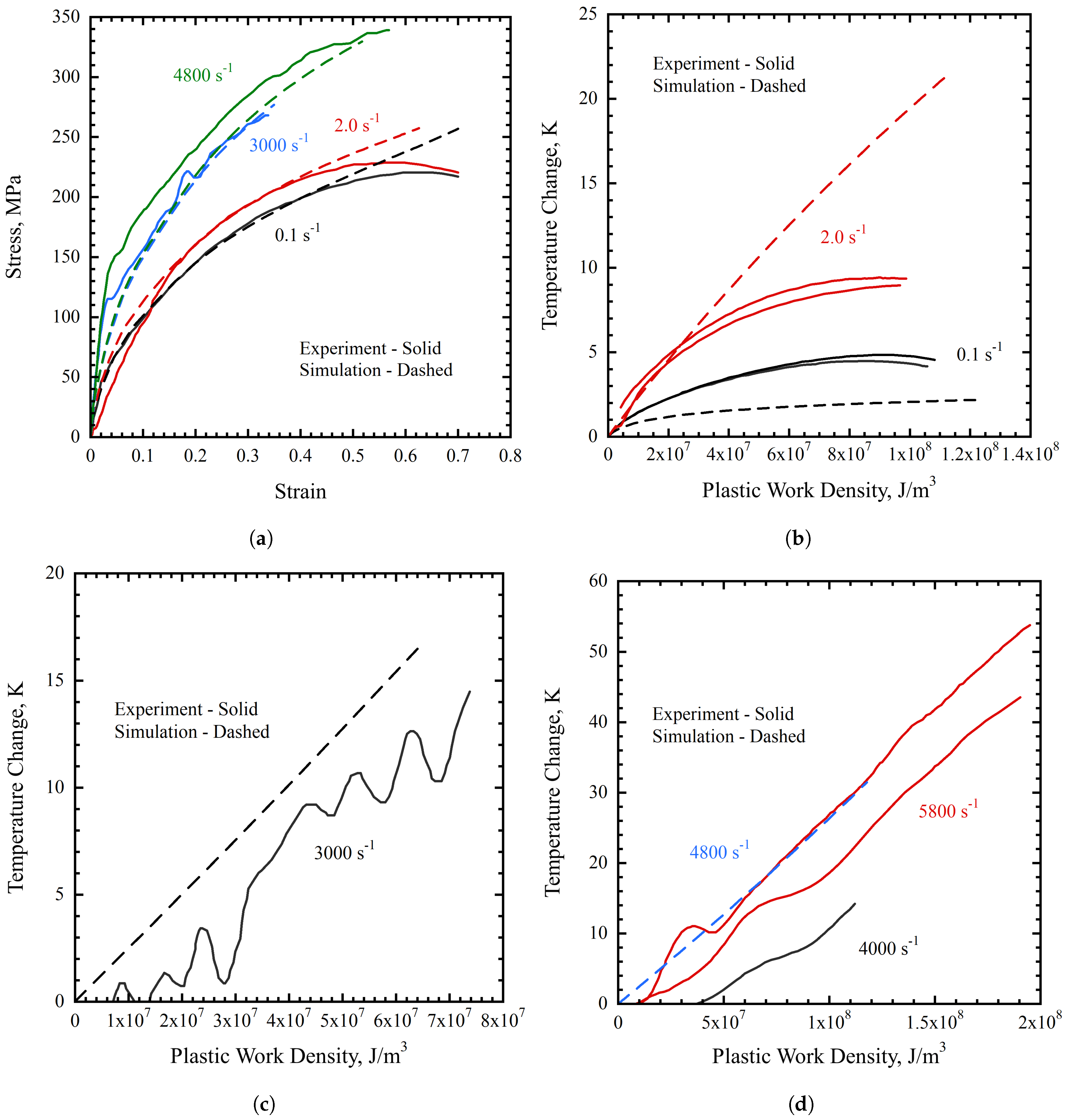
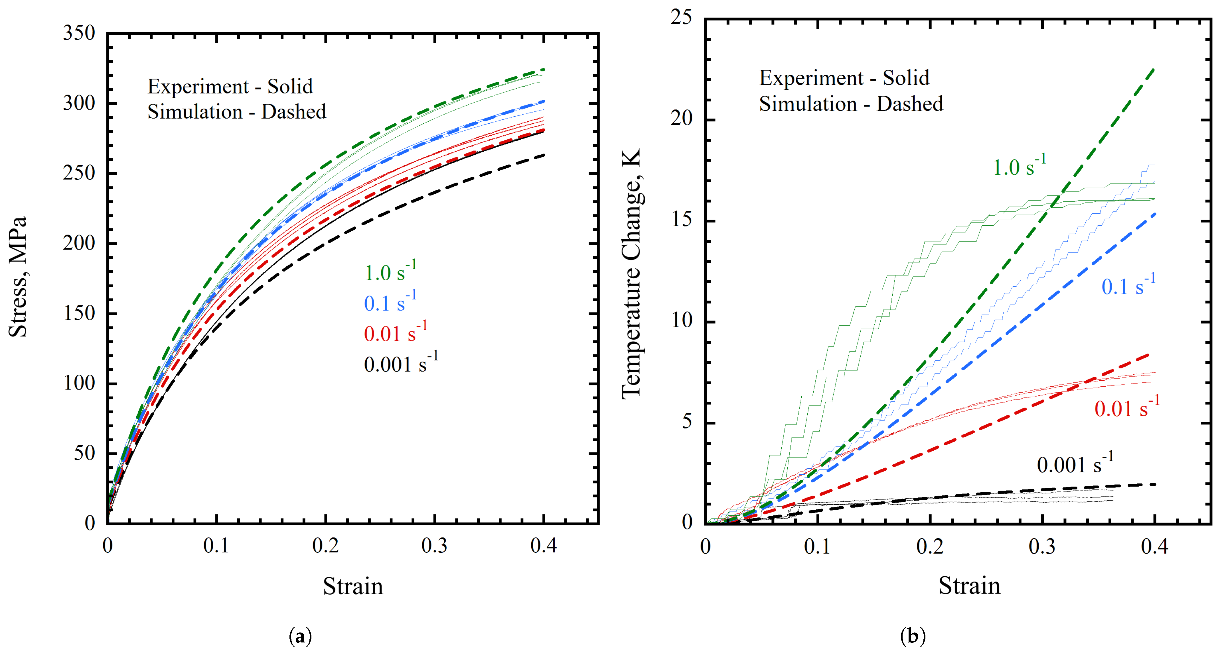
The film coefficient for air governing the transport of heat across the curved surface of the cylinder is assumed to be equal to 10.0 W/m²-K for the single crystal simulations. This is consistent with prior computational results for room-temperature experiments conducted in air. There is uncertainty in the value of the film coefficient, as seen in [77], which uses a value of 3.0 W/m²-K, and [89], which shows a wide range of values for the film coefficient (up to 13.0 W/m²-K). For the polycrystal experiments presented here, each sample was deformed to the target strain at a constant true strain rate and held under load while measuring the thermal transient cooling. This allowed for determination of the film coefficient for the conditions of these experiments. A value of 0.18 W/m²-K was determined to be suitable using results from the 0.1 ${\mathrm{s}}^{-1}$ experiments, as demonstrated in Figure 2.

3. Results

A comparison of the experimental and simulation stress–strain curves for single-crystal compression is shown in Figure 3a, demonstrating reasonable agreement between simulation and experiment. There is divergence between the simulation and experimental results for the two lower deformation rates at large strain values. Because the deformed sample shapes were not reported in [13], it is difficult to diagnose the observed softening response. As the simulations suggest strong sample distortion with deformation, it is possible that strong shear localization occurred in the experiments but was not captured by the mesh used in the simulations. Similarly, for the polycrystal case, Figure 4a shows a reasonable representation of the experimental stress–strain curves by the simulations. However, the deformation rate sensitivity of the material in the simulations is too strong in comparison with the experiments.

As expected, the single-crystal temperature curves in Figure 3b–d show high dependence of the temperature evolution behavior on the strain rate. The images corresponding to the two higher strain rate simulations (3000 ${\mathrm{s}}^{-1}$ and 4800 ${\mathrm{s}}^{-1}$) are shown in Figure 3c,d respectively. The polycrystal temperature curves in Figure 4b for the simulations show a reasonably accurate prediction of the thermocouple-measured temperature evolution in the experiments. However, a variation in the curvature of each result can be seen as a function of evolved strain. There is qualitative agreement in the strain rate sensitivity of the thermal behavior of the model, and it is again in reasonably good agreement with the experimental results. The difference in the character of the simulation and experimental temperature evolution curves suggests that some uncertainty remains in the temperature measurement as well as in our physical understanding of this thermodynamic process. Nonetheless, order-of-magnitude agreement can be seen with the simple theory used here.

The deformed shapes of the domains of the single crystal simulations for the four different strain rates are shown in Figure 5 (showing von Mises stress) and Figure 6 (showing absolute temperature). The deformed shape of the domain and contour plots for the von Mises stress and temperature show the anisotropy and heterogeneity of the deformation. Anisotropy is shown by the cross-section of the cylindrical domain, which has transformed from a circular to an elliptical shape. Heterogeneity is shown by the shearing visible in the deformed shape domains, made clearer by the patterns of the contour plots.

The predicted evolution of the Taylor–Quinney factor for both single-crystal models (Figure 7a) and polycrystal models (Figure 7b) demonstrates mild influence of the strain rate. There is clearly a strain effect on the Taylor–Quinney factor, with the Taylor–Quinney factor increasing with strain as expected. A trend appears with respect to the strain rate, however, where the Taylor–Quinney factor is lower for higher strain rates at the beginning of the simulation. With deformation, the evolution of the Taylor–Quinney factor for the higher strain rates catches up to and then exceeds the values for lower strain rates. The evolution of $\chi$ and ${\chi }_{ss}$ can be seen in Figure 7c,d, respectively.

4. Discussion

The finite deformation theory presented here has demonstrated some success in representing the experimental results. It represents dislocation interactions which are specific to the interacting slip system dislocations for face-centered cubic materials, an approach motivated by the study of these interactions with discrete dislocation dynamics and molecular dynamics calculations [36,37,38,43,80,87,88]. This is represented by a tensorial interaction within the classical Taylor expression for interaction resistance to glide. The evolution of material state in this thermodynmaic theory is also driven by plastic power, as opposed to simply the kinematic quantity of plastic slip or plastic strain rate [59,60,61,62,73,75,76]. The partitioning of plastic power into configurational and kinetic–vibrational categories affords the opportunity to suggest the coupling between plastic power and the proportion going to increasing the temperature of the material. Especially for high deformation rate loading conditions, the change in material temperature during deformation cannot be ignored; our physical mechanistic understanding of this process is quite weak. It follows that the Taylor–Quinney factor expression used here is only suggested by thermodynamics restrictions as one of the most simple admissible approaches. While such an expression is not void of physical insight, it represents a simple expression given the complexity of dislocation mechanics and the partitioning of energy in such material systems. Certainly, atomistic tools are an important avenue for gaining more physical insight into thermodynamics and physics of dislocation motion. There is also a possibility of comparing the results from the current theory with molecular dynamics simulation results, considering the advanced potential of recent developments [90]. However, such a direct comparison is difficult, as there is a large difference between the high strain rates typically necessary for MD calculations and the significantly lower strain rates of achievable polycrystal experiments and simulations. The metadynamics method developed by [91,92] may also be able to sample the potential energy landscape much more efficiently and extend the feasible strain rate regime down by many orders of magnitude. The continuum model in this work uses an Arrhenius-type flow rule based on thermal activation, and is not currently formulated for phonon drag regimes of dislocation velocity, though this could certainly be added as required [40]. As a result, the mechanical response of the continuum model is expected to match that of molecular dynamics simulation for face-centered cubic materials. The possibility of agreement of the thermal response is less certain; this flow rule physically describes the mechanical behavior of mobile dislocations but not their thermal coupling, as the exact physical basis of this coupling is not understood. However, there is much physical insight to be gained by controlled atomistic studies of this process, given the wealth of results which have already been produced.

From the polycrystal temperature evolution curves in Figure 4b, we see qualitative agreement in the strain rate behavior between experiment and simulation. The differences in curvature between the curves raise questions about the estimation of the thermal power generated in the model and the thermal energy lost to the surroundings through the boundary. It is also reasonable to expect that deformation may bring about changes in the thermocouple contact with the sample, as the bead weld area on the sample is deforming as well. Again, this highlights the challenges associated with measuring temperature for large deformation conditions, especially for high deformation rates. For the Taylor polycrystal model, the thermal power at an element integration point was calculated by averaging over the thermal power generation of all 500 single-crystal orientations active at the element integration point. What is missed in this simple homogenization approach is intergranular interactions with deformation and corresponding inhomogeneous deformation field at the single-crystal and lower length scales. This is thought to produce a greater degree of local plastic deformation, which may be missed by homogenization. On the other hand, the Taylor homogenization technique is known to be an upper bound for stress response. However, as the single-crystal and polycrystal stress–strain response is well represented, the homogenized energy should be consistent with that imposed experimentally. Then, the question is to what extent the local inhomogeneous deformation alters the energy partitioning process. Although the present results reasonably represent the experimental data, they do not address questions of the role this may play in the thermodynamic process and observations of temperature change. This has practical implication for how to approach these questions, as combined thermomechanics calculations are costly and performing sample-sized simulations (even very small samples) with realistic microstructures would be quite resource challenging even for advanced computational architectures.

The calculation of the single-crystal Taylor–Quinney factor for Figure 7a was performed by taking the average of the Taylor–Quinney factor of all the integration points in the 3D cylindrical model. This was necessary due to the highly anisotropic nature of the deformation field, as shown in Figure 5 and Figure 6. This is also consistent with the experiments due to using the entire field of thermal imaging [13]. For the polycrystal model, the deformation field is uniform, and as such the Taylor–Quinney factor was determined by averaging over all 500 crystals at the integration point nearest to the top right-hand corner node, which corresponded to the thermocouple location on the experimental samples. The polycrystal Taylor–Quinney factor evolution is provided in Figure 7b. In general, the Taylor–Quinney factor increases with deformation; however, the actual values in Figure 7a,b show that there is not much change in the predicted value over the considered range of deformations. It is, however, interesting to note that the difference in magnitude of the Taylor–Quinney factor between the single-crystal and polycrystal predictions is larger for the polycrystal by a factor of two. As mentioned earlier, the orientation of the single crystal was chosen to ensure that something close to single slip could be achieved. This produced a flow stress of 200 MPa at a strain of −0.4, in comparison with 300 MPa for the polycrystal samples for a strain rate of 0.1 ${\mathrm{s}}^{-1}$ for both datasets. The polycrystal temperature prediction for that strain rate represents the experimental curves rather well. The single-crystal prediction of temperature for that strain rate is approximately half of the experimental magnitude, indicating that perhaps the predicted single-crystal Taylor–Quinney factor is too low. The single-crystal temperature significantly overpredicts that of the experiment for a strain rate of 2.0 ${\mathrm{s}}^{-1}$. It should be noted that the boundary conditions for the single-crystal experiments were not reported by [13], and consequently those employed here for modeling these results may not be quite correct.

Although mechanical size effects are becoming more prominent features in advanced crystal mechanics theories, this was not considered in the present work. As already discussed, coupled thermomechanics problems have an implicit size effect which appears in the thermal transport component of the problem. Mechanical size effects may be introduced in various ways. Size effects related to plasticity may be introduced by calculating the dislocation density at an element integration point from the plastic part of the deformation gradient. This would necessarily require calculation of the gradient of the plastic part of the deformation gradient, and would introduce a size effect into the continuum model. Size effects related to the elastic part of the response can be introduced by assuming the material to be a micromorphic continuum. These are additional valid elements of physics which may contribute to this thermomechanical problem, and should be pursued; however, as alluded to already, adding more length scales to this study would also add substantial computational expense, and must be done with specific physics questions in mind. Given our significant remaining questions about the thermomechanical response of materials and partitioning of mechanical power, we consider it premature to include mechanical size effects at the present time, as there are higher-priority outstanding questions.

The results presented here suggest that there remains some uncertainty in the accurate measurement of temperature for the loading conditions considered here. As demonstrated in Figure 4b, the temperature evolution curves demonstrate differences in character between the different strain rate conditions. While there is good repeatability between the duplicate experiments at the same loading conditions, the curvature of the curves (with the exception of the 0.1 ${\mathrm{s}}^{-1}$ conditions, which compare well with the simulations) are not understood at present. It is also clearly important to quantify the thermal boundary conditions, which remains an opportunity for further development. This will again require close examination in the future. This is clearly an area for opportunity, as measured temperature is a critical state variable in this area of study.

5. Conclusions

We have presented an integrated study of the thermomechanical behavior of copper which includes new theoretical, computational, and experimental results. The primary variable of interest in this work is the strain rate (or time, in the context of thermal transport), which spanned the range from ${10}^{-3}$ to $5\times {10}^3$ ${\mathrm{s}}^{-1}$. All conditions were initially at room temperature. The theory and corresponding thermomechanical simulations demonstrated reasonably good agreement with the experimental results for both stress and temperature evolution, given the simplicity of the model and that there is much that we do not yet understand about the coupled thermomechanics of plastic deformation, mechanistic energy partitioning, and thermal energy conversion. The theory is formulated with large deformation kinematics, is thermodynamically consistent, and accounts for plastic power partitioning to stored energy of cold work within the dislocation structure and thermal energy of the material system. The theory accounts for advanced dislocation interaction via the continuum theory and plastic power driving structural evolution, rather than kinematical quantities such as slip rate. The dislocation interaction energy is not yet directly represented, instead being implicitly represented through material hardening as a result of dislocation interactions. Configurations of dislocation structure development such as dislocation subcells are not yet directly represented in this theory.

The single-crystal results presented here using experiments found in the literature [13] are a very important component in developing an understanding of polycrystalline thermomechanical behavior. The deformation fields at the single-crystal length scale within polycrystalline aggregates are more complex, and there does not yet exist a good way to experimentally quantify the influence of multiple grain boundary types on the deformation behavior of individual single crystals. More coupled diagnostic thermomechanical experiments performed on single crystals are needed.

The theory presented here has been used against the presented polycrystalline dataset by employing the Taylor model to homogenize the response of a representative set of 500 crystals of annealed copper with random initial crystallographic orientations. In such a treatment, each grain experiences the same imposed deformation gradient for each time step. However, depending upon its crystallographic orientation with respect the problem boundary conditions, each grain responds in a different way kinetically. The homogenized result for the simulations is then the numerical average kinetic response of each crystal, as done here, although weighted averages can also be taken. This is a reasonable first step with this new theory, and the numerical results provide a reasonable representation. Of course, intergranular interactions are an important part of the deformation response of polycrystalline metallic materials, and this remains an important question to explore.

References

1. Taylor, G.I.; Quinney, H. The latent energy remaining in a metal after cold working. Proc. R. Soc. Lond. Ser. A Contain. Pap. A Math. Phys. Character 1934, 143, 307–326. [Google Scholar]
2. Farren, W.S.; Taylor, G.I. The heat developed during plastic extension of metals. Proc. R. Soc. Lond. Ser. A Contain. Pap. A Math. Phys. Character 1925, 107, 422–451. [Google Scholar]
3. Barton, N.; Benson, D.; Becker, R. Crystal level continuum modelling of phase transformations: The α↔ϵ transformation in iron. Model. Simul. Mater. Sci. Eng. 2005, 13, 707. [Google Scholar] [CrossRef]
4. Feng, B.; Bronkhorst, C.A.; Addessio, F.L.; Morrow, B.M.; Li, W.; Lookman, T.; Cerreta, E.K. Coupled nonlinear elasticity, plastic slip, twinning, and phase transformation in single crystal titanium for plate impact loading. J. Mech. Phys. Solids 2019, 127, 358–385. [Google Scholar] [CrossRef]
5. Bronkhorst, C.A.; Gray, G.; Addessio, F.L.; Livescu, V.; Bourne, N.; McDonald, S.; Withers, P. Response and representation of ductile damage under varying shock loading conditions in tantalum. J. Appl. Phys. 2016, 119, 085103. [Google Scholar] [CrossRef]
6. Mason, J.; Rosakis, A.; Ravichandran, G. On the strain and strain rate dependence of the fraction of plastic work converted to heat: An experimental study using high speed infrared detectors and the Kolsky bar. Mech. Mater. 1994, 17, 135–145. [Google Scholar] [CrossRef]
7. Rittel, D.; Wang, Z. Thermo-mechanical aspects of adiabatic shear failure of AM50 and Ti6Al4V alloys. Mech. Mater. 2008, 40, 629–635. [Google Scholar] [CrossRef]
8. Benzerga, A.; Bréchet, Y.; Needleman, A.; Van der Giessen, E. The stored energy of cold work: Predictions from discrete dislocation plasticity. Acta Mater. 2005, 53, 4765–4779. [Google Scholar] [CrossRef]
9. Rittel, D.; Zhang, L.; Osovski, S. The dependence of the Taylor–Quinney coefficient on the dynamic loading mode. J. Mech. Phys. Solids 2017, 107, 96–114. [Google Scholar] [CrossRef]
10. Rittel, D.; Ravichandran, G.; Venkert, A. The mechanical response of pure iron at high strain rates under dominant shear. Mater. Sci. Eng. A 2006, 432, 191–201. [Google Scholar] [CrossRef]
11. Rittel, D.; Bhattacharyya, A.; Poon, B.; Zhao, J.; Ravichandran, G. Thermomechanical characterization of pure polycrystalline tantalum. Mater. Sci. Eng. A 2007, 447, 65–70. [Google Scholar] [CrossRef]
12. Rittel, D.; Silva, M.; Poon, B.; Ravichandran, G. Thermomechanical behavior of single crystalline tantalum in the static and dynamic regime. Mech. Mater. 2009, 41, 1323–1329. [Google Scholar] [CrossRef]
13. Rittel, D.; Kidane, A.; Alkhader, M.; Venkert, A.; Landau, P.; Ravichandran, G. On the dynamically stored energy of cold work in pure single crystal and polycrystalline copper. Acta Mater. 2012, 60, 3719–3728. [Google Scholar] [CrossRef]
14. Asaro, R.J.; Rice, J. Strain localization in ductile single crystals. J. Mech. Phys. Solids 1977, 25, 309–338. [Google Scholar] [CrossRef]
15. Asaro, R.J. Crystal plasticity. J. Appl. Mech. 1983, 50, 921–934. [Google Scholar] [CrossRef]
16. Asaro, R.J. Micromechanics of crystals and polycrystals. Adv. Appl. Mech. 1983, 23, 1–115. [Google Scholar]
17. Asaro, R.J.; Needleman, A. Overview no. 42 texture development and strain hardening in rate dependent polycrystals. Acta Metall. 1985, 33, 923–953. [Google Scholar] [CrossRef]
18. Bassani, J.L. Plastic flow of crystals. Adv. Appl. Mech. 1993, 30, 191–258. [Google Scholar]
19. Bassani, J.L.; Wu, T.Y. Latent hardening in single crystals. II. Analytical characterization and predictions. Proc. R. Soc. Lond. Ser. A Math. Phys. Sci. 1991, 435, 21–41. [Google Scholar]
20. Wu, T.Y.; Bassani, J.L.; Laird, C. Latent hardening in single crystals-I. Theory and experiments. Proc. R. Soc. Lond. Ser. A Math. Phys. Sci. 1991, 435, 1–19. [Google Scholar]
21. Kalidindi, S.R.; Bronkhorst, C.A.; Anand, L. Crystallographic texture evolution in bulk deformation processing of FCC metals. J. Mech. Phys. Solids 1992, 40, 537–569. [Google Scholar] [CrossRef]
22. Bronkhorst, C.A.; Kalidindi, S.; Anand, L. Polycrystalline plasticity and the evolution of crystallographic texture in FCC metals. Philos. Trans. R. Soc. Lond. Ser. A Phys. Eng. Sci. 1992, 341, 443–477. [Google Scholar]
23. Harren, S.; Asaro, R. Nonuniform deformations in polycrystals and aspects of the validity of the Taylor model. J. Mech. Phys. Solids 1989, 37, 191–232. [Google Scholar] [CrossRef]
24. Harren, S.; Lowe, T.C.; Asaro, R.J.; Needleman, A. Analysis of large-strain shear in rate-dependent face-centred cubic polycrystals: Correlation of micro-and macromechanics. Philos. Trans. R. Soc. Lond. Ser. A Math. Phys. Sci. 1989, 328, 443–500. [Google Scholar]
25. Acharya, A.; Tang, H.; Saigal, S.; Bassani, J.L. On boundary conditions and plastic strain-gradient discontinuity in lower-order gradient plasticity. J. Mech. Phys. Solids 2004, 52, 1793–1826. [Google Scholar] [CrossRef]
26. Aifantis, E.C. On the role of gradients in the localization of deformation and fracture. Int. J. Eng. Sci. 1992, 30, 1279–1299. [Google Scholar] [CrossRef]
27. Anand, L.; Gurtin, M.; Lele, S.; Gething, C. A one-dimensional theory of strain-gradient plasticity: Formulation, analysis, numerical results. J. Mech. Phys. Solids 2005, 53, 1789–1826. [Google Scholar] [CrossRef]
28. Arsenlis, A.; Parks, D. Crystallographic aspects of geometrically-necessary and statistically-stored dislocation density. Acta Mater. 1999, 47, 1597–1611. [Google Scholar] [CrossRef]
29. Busso, E.P.; McClintock, F.A. A dislocation mechanics-based crystallographic model of a B2-type intermetallic alloy. Int. J. Plast. 1996, 12, 1–28. [Google Scholar] [CrossRef]
30. Busso, E.; Meissonnier, F.; O’Dowd, N. Gradient-dependent deformation of two-phase single crystals. J. Mech. Phys. Solids 2000, 48, 2333–2361. [Google Scholar] [CrossRef]
31. Gerken, J.M.; Dawson, P.R. A crystal plasticity model that incorporates stresses and strains due to slip gradients. J. Mech. Phys. Solids 2008, 56, 1651–1672. [Google Scholar] [CrossRef]
32. Gurtin, M.E. On the plasticity of single crystals: Free energy, microforces, plastic-strain gradients. J. Mech. Phys. Solids 2000, 48, 989–1036. [Google Scholar] [CrossRef]
33. Gurtin, M.E.; Needleman, A. Boundary conditions in small-deformation, single-crystal plasticity that account for the Burgers vector. J. Mech. Phys. Solids 2005, 53, 1–31. [Google Scholar] [CrossRef]
34. Mayeur, J.; Beyerlein, I.; Bronkhorst, C.; Mourad, H. Incorporating interface affected zones into crystal plasticity. Int. J. Plast. 2015, 65, 206–225. [Google Scholar] [CrossRef]
35. Zhu, H.; Zbib, H. On the role of strain gradients in adiabatic shear banding. Acta Mech. 1995, 111, 111–124. [Google Scholar] [CrossRef]
36. Dequiedt, J.; Denoual, C.; Madec, R. Heterogeneous deformation in ductile FCC single crystals in biaxial stretching: The influence of slip system interactions. J. Mech. Phys. Solids 2015, 83, 301–318. [Google Scholar] [CrossRef]
37. Devincre, B.; Kubin, L.; Hoc, T. Physical analyses of crystal plasticity by DD simulations. Scr. Mater. 2006, 54, 741–746. [Google Scholar] [CrossRef]
38. Devincre, B.; Hoc, T.; Kubin, L. Dislocation Mean Free Paths and Strain Hardening of Crystals. Science 2008, 320, 1745–1748. [Google Scholar] [CrossRef]
39. Grilli, N.; Janssens, K.; Nellessen, J.; Sandlöbes, S.; Raabe, D. Multiple slip dislocation patterning in a dislocation-based crystal plasticity finite element method. Int. J. Plast. 2018, 100, 104–121. [Google Scholar] [CrossRef]
40. Hansen, B.; Beyerlein, I.; Bronkhorst, C.; Cerreta, E.; Dennis-Koller, D. A dislocation-based multi-rate single crystal plasticity model. Int. J. Plast. 2013, 44, 129–146. [Google Scholar] [CrossRef]
41. Hansen, B.; Bronkhorst, C.; Ortiz, M. Dislocation subgrain structures and modeling the plastic hardening of metallic single crystals. Model. Simul. Mater. Sci. Eng. 2010, 18, 055001. [Google Scholar] [CrossRef]
42. Lee, S.; Cho, H.; Bronkhorst, C.A.; Pokharel, R.; Brown, D.W.; Clausen, B.; Vogel, S.C.; Anghel, V.; Gray, G.T.; Mayeur, J.R. Deformation, dislocation evolution and the non-Schmid effect in body-centered-cubic single- and polycrystal tantalum. Int. J. Plast. 2023, 163, 103529. [Google Scholar] [CrossRef]
43. Madec, R.; Kubin, L.P. Dislocation strengthening in FCC metals and in BCC metals at high temperatures. Acta Mater. 2017, 126, 166–173. [Google Scholar] [CrossRef]
44. Nguyen, T.; Fensin, S.J.; Luscher, D.J. Dynamic crystal plasticity modeling of single crystal tantalum and validation using Taylor cylinder impact tests. Int. J. Plast. 2021, 139, 102940. [Google Scholar] [CrossRef]
45. Butler, B.G.; Paramore, J.D.; Ligda, J.P.; Ren, C.; Fang, Z.Z.; Middlemas, S.C.; Hemker, K.J. Mechanisms of deformation and ductility in tungsten—A review. Int. J. Refract. Met. Hard Mater. 2018, 75, 248–261. [Google Scholar] [CrossRef]
46. Feng, B.; Bronkhorst, C.; Addessio, F.; Morrow, B.; Cerreta, E.; Lookman, T.; Lebensohn, R.; Low, T. Coupled elasticity, plastic slip, and twinning in single crystal titanium loaded by split-Hopkinson pressure bar. J. Mech. Phys. Solids 2018, 119, 274–297. [Google Scholar] [CrossRef]
47. Acharya, A. New inroads in an old subject: Plasticity, from around the atomic to the macroscopic scale. J. Mech. Phys. Solids 2010, 58, 766–778. [Google Scholar] [CrossRef]
48. Anand, L.; Gurtin, M.E.; Reddy, B.D. The stored energy of cold work, thermal annealing, and other thermodynamic issues in single crystal plasticity at small length scales. Int. J. Plast. 2015, 64, 1–25. [Google Scholar] [CrossRef]
49. Arora, R.; Acharya, A. Dislocation pattern formation in finite deformation crystal plasticity. Int. J. Solids Struct. 2020, 184, 114–135. [Google Scholar] [CrossRef]
50. Berdichevsky, V. Why is classical thermodynamics insufficient for solids? In Proceedings of the 2018 AIAA/ASCE/AHS/ASC Structures, Structural Dynamics, and Materials Conference, Kissimmee, FL, USA, 8–12 January 2018. [CrossRef]
51. Berdichevsky, V. A continuum theory of edge dislocations. J. Mech. Phys. Solids 2017, 106, 95–132. [Google Scholar] [CrossRef]
52. Berdichevsky, V. Entropy and temperature of microstructure in crystal plasticity. Int. J. Eng. Sci. 2018, 128, 24–30. [Google Scholar] [CrossRef]
53. Berdichevsky, V. Beyond classical thermodynamics: Dislocation-mediated plasticity. J. Mech. Phys. Solids 2019, 129, 83–118. [Google Scholar] [CrossRef]
54. del Castillo, P.R.D.; Huang, M. Dislocation annihilation in plastic deformation: I. Multiscale irreversible thermodynamics. Acta Mater. 2012, 60, 2606–2614. [Google Scholar] [CrossRef]
55. Roy Chowdhury, S.; Roy, D. A non-equilibrium thermodynamic model for viscoplasticity and damage: Two temperatures and a generalized fluctuation relation. Int. J. Plast. 2019, 113, 158–184. [Google Scholar] [CrossRef]
56. Hochrainer, T. Thermodynamically consistent continuum dislocation dynamics. J. Mech. Phys. Solids 2016, 88, 12–22. [Google Scholar] [CrossRef]
57. Jafari, M.; Jamshidian, M.; Ziaei-Rad, S. A finite-deformation dislocation density-based crystal viscoplasticity constitutive model for calculating the stored deformation energy. Int. J. Mech. Sci. 2017, 128–129, 486–498. [Google Scholar] [CrossRef]
58. Jiang, M.; Devincre, B.; Monnet, G. Effects of the grain size and shape on the flow stress: A dislocation dynamics study. Int. J. Plast. 2019, 113, 111–124. [Google Scholar] [CrossRef]
59. Langer, J.; Bouchbinder, E.; Lookman, T. Thermodynamic theory of dislocation-mediated plasticity. Acta Mater. 2010, 58, 3718–3732. [Google Scholar] [CrossRef]
60. Langer, J.S. Statistical thermodynamics of strain hardening in polycrystalline solids. Phys. Rev. E 2015, 92, 032125. [Google Scholar] [CrossRef]
61. Le, K.; Tran, T.; Langer, J. Thermodynamic dislocation theory of adiabatic shear banding in steel. Scr. Mater. 2018, 149, 62–65. [Google Scholar] [CrossRef]
62. Le, K. Thermodynamic dislocation theory for non-uniform plastic deformations. J. Mech. Phys. Solids 2018, 111, 157–169. [Google Scholar] [CrossRef]
63. Le, K. Thermodynamic dislocation theory: Finite deformations. Int. J. Eng. Sci. 2019, 139, 1–10. [Google Scholar] [CrossRef]
64. Le, K.C.; Tran, T.M.; Langer, J.S. Thermodynamic dislocation theory of high-temperature deformation in aluminum and steel. Phys. Rev. E 2017, 96, 013004. [Google Scholar] [CrossRef] [PubMed]
65. Levitas, V.I.; Javanbakht, M. Thermodynamically consistent phase field approach to dislocation evolution at small and large strains. J. Mech. Phys. Solids 2015, 82, 345–366. [Google Scholar] [CrossRef]
66. Nieto-Fuentes, J.; Rittel, D.; Osovski, S. On a dislocation-based constitutive model and dynamic thermomechanical considerations. Int. J. Plast. 2018, 108, 55–69. [Google Scholar] [CrossRef]
67. Po, G.; Huang, Y.; Ghoniem, N. A continuum dislocation-based model of wedge microindentation of single crystals. Int. J. Plast. 2019, 114, 72–86. [Google Scholar] [CrossRef]
68. Roy, A.; Acharya, A. Finite element approximation of field dislocation mechanics. J. Mech. Phys. Solids 2005, 53, 143–170. [Google Scholar] [CrossRef]
69. Roy, A.; Acharya, A. Size effects and idealized dislocation microstructure at small scales: Predictions of a Phenomenological model of Mesoscopic Field Dislocation Mechanics: Part II. J. Mech. Phys. Solids 2006, 54, 1711–1743. [Google Scholar] [CrossRef]
70. Shizawa, K.; Kikuchi, K.; Zbib, H.M. A strain-gradient thermodynamic theory of plasticity based on dislocation density and incompatibility tensors. Mater. Sci. Eng. A 2001, 309-310, 416–419. [Google Scholar] [CrossRef]
71. Clayton, J. Nonlinear thermomechanics for analysis of weak shock profile data in ductile polycrystals. J. Mech. Phys. Solids 2019, 124, 714–757. [Google Scholar] [CrossRef]
72. Clayton, J.D. Nonlinear Mechanics of Crystals; Springer Science & Business Media: Berlin/Heidelberg, Germany, 2010; Volume 177. [Google Scholar]
73. Langer, J.S. Thermal effects in dislocation theory. Phys. Rev. E 2016, 94, 063004. [Google Scholar] [CrossRef] [PubMed]
74. Langer, J. Statistical thermodynamics of dislocations in solids. Adv. Phys. 2021, 70, 445–467. [Google Scholar] [CrossRef]
75. Lieou, C.K.; Bronkhorst, C.A. Dynamic recrystallization in adiabatic shear banding: Effective-temperature model and comparison to experiments in ultrafine-grained titanium. Int. J. Plast. 2018, 111, 107–121. [Google Scholar] [CrossRef]
76. Lieou, C.K.; Mourad, H.M.; Bronkhorst, C.A. Strain localization and dynamic recrystallization in polycrystalline metals: Thermodynamic theory and simulation framework. Int. J. Plast. 2019, 119, 171–187. [Google Scholar] [CrossRef]
77. Lieou, C.K.; Bronkhorst, C.A. Thermomechanical conversion in metals: Dislocation plasticity model evaluation of the Taylor-Quinney coefficient. Acta Mater. 2021, 202, 170–180. [Google Scholar] [CrossRef]
78. Lieou, C.K.; Bronkhorst, C.A. Thermodynamic theory of crystal plasticity: Formulation and application to polycrystal fcc copper. J. Mech. Phys. Solids 2020, 138, 103905. [Google Scholar] [CrossRef]
79. Noll, W.; Coleman, B.D.; Noll, W. The thermodynamics of elastic materials with heat conduction and viscosity. In The Foundations of Mechanics and Thermodynamics: Selected Papers; Springer: Berlin/Heidelberg, Germany, 1974; pp. 145–156. [Google Scholar]
80. Kubin, L.; Devincre, B.; Hoc, T. Modeling dislocation storage rates and mean free paths in face-centered cubic crystals. Acta Mater. 2008, 56, 6040–6049. [Google Scholar] [CrossRef]
81. Bronkhorst, C.; Hansen, B.; Cerreta, E.; Bingert, J. Modeling the microstructural evolution of metallic polycrystalline materials under localization conditions. J. Mech. Phys. Solids 2007, 55, 2351–2383. [Google Scholar] [CrossRef]
82. Hansen, B.; Carpenter, J.; Sintay, S.; Bronkhorst, C.; McCabe, R.; Mayeur, J.; Mourad, H.; Beyerlein, I.; Mara, N.; Chen, S.; et al. Modeling the texture evolution of Cu/Nb layered composites during rolling. Int. J. Plast. 2013, 49, 71–84. [Google Scholar] [CrossRef]
83. Mayeur, J.; Beyerlein, I.; Bronkhorst, C.; Mourad, H.; Hansen, B. A crystal plasticity study of heterophase interface character stability of Cu/Nb bicrystals. Int. J. Plast. 2013, 48, 72–91. [Google Scholar] [CrossRef]
84. Kocks, U. Laws for work-hardening and low-temperature creep. J. Eng. Mater. Technol. 1976, 98, 76–85. [Google Scholar] [CrossRef]
85. Balasubramanian, S. Polycrystalline Plasticity: Application to Deformation Processing of Lightweight Metals. Ph.D. Thesis, Massachusetts Institute of Technology, Cambridge, MA, USA, 1998. [Google Scholar]
86. Simmons, G.; Wang, H. Single Crystal Elastic Constants and Calculated Aggregate Properties: A Handbook; The M.I.T. Press: Cambridge, MA, USA, 1971. [Google Scholar]
87. Madec, R.; Devincre, B.; Kubin, L.P. From dislocation junctions to forest hardening. Phys. Rev. Lett. 2002, 89, 255508. [Google Scholar] [CrossRef] [PubMed]
88. Madec, R.; Devincre, B.; Kubin, L.; Hoc, T.; Rodney, D. The role of collinear interaction in dislocation-induced hardening. Science 2003, 301, 1879–1882. [Google Scholar] [CrossRef] [PubMed]
89. Awbi, H.B. Calculation of convective heat transfer coefficients of room surfaces for natural convection. Energy Build. 1998, 28, 219–227. [Google Scholar] [CrossRef]
90. Owen, C.J.; Naghdi, A.D.; Johansson, A.; Massa, D.; Papanikolaou, S.; Kozinsky, B. Unbiased Atomistic Predictions of Crystal Dislocation Dynamics using Bayesian Force Fields. arXiv 2024, arXiv:2401.04359. [Google Scholar]
91. Fan, Y.; Kushima, A.; Yip, S.; Yildiz, B. Mechanism of Void Nucleation and Growth in bcc Fe: Atomistic Simulations at Experimental Time Scales. Phys. Rev. Lett. 2011, 106, 125501. [Google Scholar] [CrossRef]
92. Fan, Y.; Yip, S.; Yildiz, B. Autonomous basin climbing method with sampling of multiple transition pathways: Application to anisotropic diffusion of point defects in hcp Zr. J. Phys. Condens. Matter 2014, 26, 365402. [Google Scholar] [CrossRef]
Figure 1. Meshes representing initial configurations: (a) single-crystal, sample size of 6mm diameter and 6 mm length; (b) axisymmetric and half-length thermomechanical polycrystal mesh (sample size of 12.7 mm diameter and 19.05 mm length), where the left edge is the axis of symmetry, the top edge is the sample’s center, the bottom (tan) region corresponds to steel platens (9.34 mm height, 6.35 mm width), the top (green) region corresponds to copper (9.525 mm height), and a thin (0.0127 mm) PTFE layer is between the steel and copper; (c) axisymmetric and half-length thermal transient model.
Metals 14 01086 g001
Figure 2. Temperature transient results used to determine a numerical film coefficient for the air–solid interface of 0.18 W/m2-K. The temperature measured by the thermocouples and simulated temperature are taken from the center surface node.
Metals 14 01086 g002
Figure 3. Comparison of experiment and simulation for single-crystal copper. Solid lines represent experiments and dashed lines represent simulations. Plastic work densities are calculated as the area under the stress–strain curve. The simulation temperature change was taken from the center surface node. (a) Single crystal stress–strain; (b) 0.1 s 1 and 2.0 s 1 temperature change; (c) 3000 s 1 temperature change; (d) 4000 s 1 and 5800 s 1 temperature changes.
Metals 14 01086 g003
Figure 4. Comparison of polycrystal experiment and simulation results: (a) stress-strain curve for polycrystal copper and (b) temperature evolution for polycrystal copper. The experimental temperature was measured by thermocouples, while the simulated temperature was taken from the center surface node.
Metals 14 01086 g004
Figure 5. Deformed shapes of single-crystal simulations, showing the von Mises stress for different strain rates: (a), ϵ ˙ = 0.1   s 1 ; (b) ϵ ˙ = 2   s 1 ; (c) ϵ ˙ = 3000   s 1 ; (d) ϵ ˙ = 4800   s 1 . All images were taken at an axial compressive strain of 0.35. The von Mises stress, also known as equivalent stress, is defined as σ V M = 3 / 2 T ̲ : T ̲ .
Metals 14 01086 g005
Figure 6. Deformed shapes of single-crystal simulations showing the temperature for different strain rates: (a) ϵ ˙ = 0.1   s 1 ; (b) ϵ ˙ = 2   s 1 ; (c) ϵ ˙ = 3000   s 1 ; (d) ϵ ˙ = 4800   s 1 . The initial temperature for all simulations was 295 K. All images were taken at an axial compressive strain of 0.35.
Metals 14 01086 g006
Figure 7. Evolution of Taylor-Quinney state variables for single and polycrystal simulations: (a) single-crystal Taylor-Quinney factor; (b) polycrystal Taylor-Quinney factor; (c) polycrystal effective temperature; (d) polycrystal steady-state effective temperature.
Metals 14 01086 g007