Article

Surface Reaction-Diffusion-Coupled Simulation of Ni–Fe–Cr Alloy under FLiNaK Molten Salt

1
Department of Nuclear Engineering, Kyung Hee University, Yongin-si 17104, Republic of Korea
2
Department of Materials Science and Engineering, University of Florida, Gainesville, FL 32603, USA
*
Author to whom correspondence should be addressed.
Metals 2024, 14(9), 1088; https://doi.org/10.3390/met14091088
Submission received: 14 August 2024 / Revised: 19 September 2024 / Accepted: 20 September 2024 / Published: 23 September 2024
(This article belongs to the Section Computation and Simulation on Metals)

Abstract

:
A molten salt reactor is one of the fourth-generation reactors and is considered to be a feasible replacement for current reactors due to their many advantages. However, there are a number of issues that remain; one of which is the corrosion of the materials. Corrosion problems in molten salt reactors have been reported since The Molten Salt Reactor Experiment at Oak Ridge National Laboratory in the 1960s. There have been many attempts to mitigate the corrosion problem, but a fundamental solution has not yet been achived. In this study, surface reaction-diffusion-coupled simulations were performed to simulate the corrosion of a Ni–Cr–Fe material, a prototype of Hastelloy N, which is being promoted as a structural material for molten salt reactors in F–Li–Na–K eutectic salts. This surface reaction-diffusion-coupled simulation framework was developed to study which corrosion reactions are dominant in molten salt environment corrosion where a large number of oxidation–reduction reactions exist, the correlation between composition of alloy and corrosion rate, and the effect of Cr depletion on corrosion.

1. Introduction

A molten salt reactor (hereafter MSR) is a fourth-generation reactor design that has gained significant attention for its inherent safety, due to the reactor’s negative temperature coefficient of reactivity [1,2,3], and its ability to eliminate the need for a pressurization system [2,4,5], resulting in a smaller, simpler design [2,6]. Furthermore, unlike light water reactors, there is no risk of a hydrogen explosion in the event of a LOCA (Loss Of Coolant Accident) [7,8], and the leakage of radioactive material is much smaller compared to light water reactors because the leaked coolant quickly solidifies [7,9,10].
The Molten Salt Reactor Experiment, conducted in the 1960s at Oak Ridge National Laboratory [5,6], confirmed the feasibility of molten salt reactors, but also highlighted many problems that needed improvement, one of which was the corrosion of reactor structural materials by molten salt [11,12,13,14,15].
Unlike aqueous environments, where corrosion can be prevented by a passive oxide film on the alloy surface, in molten salt environments, the oxide film is unstable and cannot be mitigated by a passive oxide film [14,16]. Additionally, corrosion can occur due to various impurities, such as fission products, moisture, and metal cations [8,17]. Moreover, temperature differences and differences in chemical potentials between different materials can accelerate corrosion [8]. Material corrosion by molten salts has been studied experimentally in stainless steels [18,19,20,21,22] and Ni-based alloys [21,22,23,24]. There are studies on complex corrosion mechanisms, and some studies use electrochemical analysis to calculate the reduction potential of the corrosion reaction [4,11]. Based on the redox potential, there are studies on corrosion mitigation by adding chemical species to be corroded instead or controlling impurities by purifying the molten salt online [15,25].
It is known that the corrosion phenomenon is governed by (1) thermodynamic factors that determine the electrode potential and (2) kinetic factors that determine the surface reaction rate. However, elements such as Li + , Na + , and K + are not thermodynamically expected to undergo reduction reactions [11], so it is still uncertain what the opposite reduction reaction to the oxidation reaction of Cr or Ni is, and the reduction reaction is assumed to be the impurity reaction, but it is still unclear which reaction is the main impurity reaction [8]. However, it is understood as an impurity-driven corrosion phenomenon, and the impurity reaction assuming the trace presence of hydrogen ions is assumed in this study.
The corrosion phenomenon in the molten salt environment of MSRs is a multiphysical phenomenon involving corrosion of materials [26], chemical reactions between substances—including fission products in the fuel salt [8,11] and the flow of fuel salt [4,8]. It requires more in-depth and extensive research for a comprehensive analysis of the phenomenon.
The development of a surface reaction-diffusion-coupled corrosion simulation framework will be an important step in the development of multiphysics simulation tools that can predict the corrosion behavior in molten salt reactors, including various physical phenomena such as flow and temperature gradients. Previous study of electrochemical reactions in molten salts using the COMSOL corrosion module has been conducted to analyze a metal electrolysis study [27], which confirmed the ability to link surface electrochemical reactions with transport equations. In this study, we performed surface reaction-diffusion-coupled corrosion simulation to evaluate the corrosion rate in Ni–Cr–Fe alloys exposed to molten FLiNaK by the composition of the alloy. Wang et al. predicted molten salt environment corrosion of Ni-based 625 alloy by performing probabilistic predictions based on cellular automata rather than solving interface reaction or diffusion equations directly [28]. Li et al. predicted the molten salt environment corrosion of a material based on first principle molecular dynamics, utilizing the Berzins–Delahay equation, which utilizes the correlation between exchange current density and impedance, instead of Butler–Volmer, which correlates the current and potential for surface reactions [29]. Bhave et al. proposed a simulation framework to predict the corrosion behavior of Ni–Cr alloys in F–Li–Be molten salts using the linearized Butler–Volmer equation [30]. Feng et al. simulated the corrosion behavior of 625 alloy in a molten salt environment with a cellular automata method and made progress in incorporating grain size effects [31]. In this study, we extended the material composition to the Ni–Cr–Fe ternary system, allowing us to consider the reduction reactions of Fe ions, and made significant progress in predicting surface reactions utilizing the full Butler–Volmer equation. The comparison between current work and previous work [30] is shown in Table 1.
In this paper, we begin by describing the model in Section 2, including the model geometry, simulation strategy, and boundary and initial conditions. In Section 3, we present the results from the model. In Section 4, we fit the mass loss of Cr with a polynomial and observe the Cr depletion effect in the simulation. Both general corrosion [8,32] and localized corrosion, such as pitting corrosion [8,32] occur in the structural materials of molten salt reactors. Among them, pitting corrosion is highly influenced by microstructural inhomogeneities such as grain boundaries [33], and this inhomogeneity is not reflected in this study, so only general corrosion is considered in this study.

2. Model Description
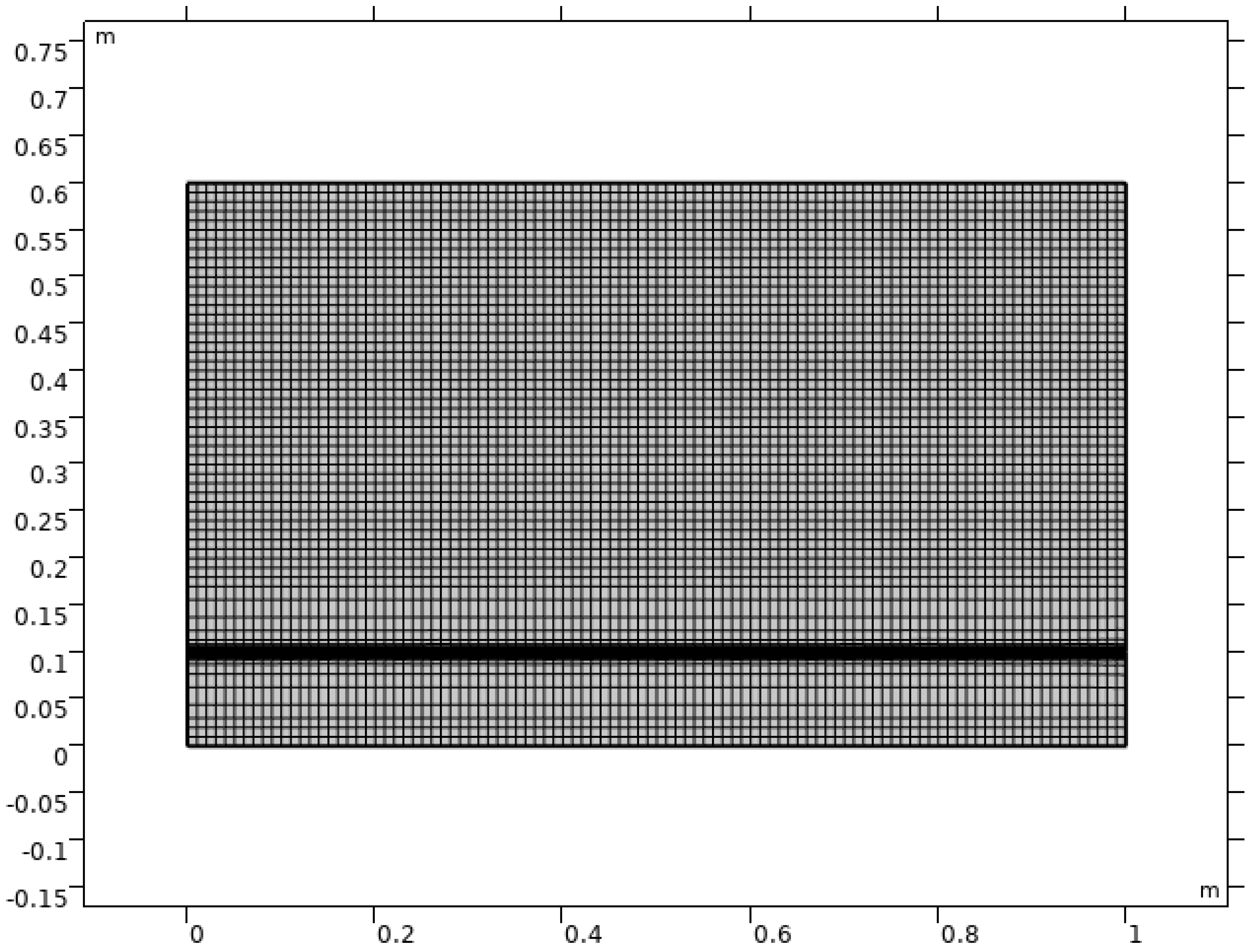
2.1. Model Geometry

The model geometry is two-dimensional rectangular geometry, as shown in Figure 1. The blue shaded area is the electrolyte region (molten salt), and all reactions are set to occur at the bottom of that region, at the interface with the electrode (alloy).
The mesh of the geometry is shown in Figure 2. The mesh size of the bulk region is 0.01   m square and interface with molten salt and the alloy region is 0.0005   m .

2.2. Simulation Strategy

We solve the Nernst–Planck equation that mainly analyzes the mass transfer of chemical species in the molten salt, and the Butler–Volmer equation that predicts the electrochemical reaction at the alloy surface. To simulate the mass transfer and electrochemical reaction, the implicit finite element method is applied using the COMSOL (6.2 version, COMSOL Inc., Burlington, MA, USA) corrosion module.
The Nernst–Planck equation, which satisfies the conservation of mass for chemical species j is provided by
c j t + · J j + u · c j = R j
where c j is the concentration of each chemical species j (mol/ m 3 ), t is the time ( s ), J j is the flux of chemical species j (mol/ m 2 · s ), u is the velocity of the molten salt ( m / s ), and R j is the source of the chemical species j (mol/ m 3 · s ).
The flux is calculated by diffusion and electromigration of the chemical species in the molten salt, and the effect of convection is included in Equation (1) as u · c j . So, the flux is provided by
J j = D j e l c j z j u m , j F c j ϕ l ,
where D j e l is the diffusion coefficient of the j chemical species in the salt ( m 2 s 1 ), z j is the charge of j chemical species, u m , j is the electromigration mobility of j chemical species ( s ·mol/ k g ), F is Faraday’s constant (C/mol), ϕ l is the electrolyte potential ( V ), and the first term on the right-hand side corresponds to diffusion and the second term to electromigration.
Electrolyte potential ( ϕ l ) is the potential that appears in the electrochemical potential of a species in the solution. Also, we cannot determine the electrolyte potential using only the Nernst–Planck equation. The number of Nernst–Plank equations is j and the number of variables is the concentration of j chemical species plus the potential of the electrolyte, totaling j + 1 . Finally, an electroneutrality condition is considered to reduce the number of dependant concentration variables by one. The electroneutrality condition is provided by
j z j c j = 0 ,
which follows from the dimensional analysis of Gauss’s law. In a typical molten salt solution, it is accurate over lengths greater than a few nanometers. Using the electroneutrality condition eliminates the need to represent one of the charge carriers, reducing the number of dependent concentration variables of the chemical species by one.
The diffusion coefficient in Equation (2) was determined using the Stokes–Einstein equation [34]:
D j e l = k B T 6 π μ r j ,
where k B is the Boltzman constant ( J / K ), T is the absolute temperature ( K ), μ is the dynamic viscosity ( Pa · s ), and r j is the radius of particle ( m ). The superscript e l means that the value is the elemental diffusion coefficient in the molten salt. Equation (4) is used to determine the diffusion coefficient of a species in a fluid with a low Reynolds number, assuming that the particles of the species are spherical. The mobility in Equation (2) is calculated from the diffusion coefficient using the Nernst–Einstein relation:
u m , j = D j e l R T ,
where R is the gas constant ( J / K ·mol). It is assumed that the current in the molten salt flows only by the movement of ions, such that the current density vector in the molten salt i l ( A / m 2 ) is the sum of the fluxes of all chemical species:
i l = F j z j J j ,
which satisfies the conservation of charge. It is computed only for chemical species j in the molten salt.
Thus far, the equations only consider mass transfer in the molten salt. Now, the governing equation for the electrochemical reaction on the alloy surface is presented. The stoichiometry coefficients for the electrochemical reaction at the alloy surface are defined as follows:
o x | v o x | S o x + n e r e d v r e d S r e d ,
where S r e d is the reduced chemical species and is the product of the reduction reaction. S o x is the oxidized species and is the reactant in the reduction reaction. v o x and v r e d are the stoichiometry coefficients of the respective species and v o x is defined as negative to distinguish whether the species is oxidized or reduced. At the surface, the oxidation reaction of the alloy and the reduction reaction of the alkali metal and impurities in the molten salt can occur, as shown in Table 2.
The stoichiometry coefficient and the number of electrons participating in the reaction are determined by substituting each reaction into Equation (7), as demonstrated in Table 3.
The molar flux ( R j , mol/ m 2 · s ) of j chemical species perpendicular to the alloy–molten salt interface is calculated as the sum of the fluxes generated by all of the electrode reactions, i.e.,
R j = m v j , m i l o c , m n m F ,
where i l o c , m is the local current density of the m reaction ( A / m 2 ), which is calculated by the mass action law Butler–Volmer equation:
i l o c , m = i 0 , m exp α a , m F η m R T exp α c , m F η m R T ,
where i 0 , m is the exchange current density of the m reaction, α a , m ( α c , m ) is the transfer constant, and η m is the overpotential. The exchange current i 0 , m includes a term for concentration and is provided by
i 0 , m = i 0 , m r e f ( T ) j : v j > 0 c j c j r e f α c , m v j n j : v j < 0 c j c j r e f α a , m v j n ,
where i 0 , m r e f is the reference exchange current density. The overpotential is provided by
η m = ϕ s ϕ l E e q , m ,
where ϕ s is the electrode potential, E e q , m is the equilibrium potential of the m reaction, and the equilibrium potential is calculated by the Nernst equation:
E e q , m = E e q , m r e f ( T ) R T n F l n j c j c j r e f v j ,
where c j r e f is reference concentration of j species and E e q , m r e f ( T ) is the reference equilibrium potential at T temperature and c j r e f concentration.
The model can be run in two ways with respect to the concentration of elements in the alloy. It can be assumed that there are an infinite supply of elements in the alloy, such that their concentrations are constant with time. Alternatively, the effect of alloy depletion from the alloy can be represented by assuming that the elements in the alloy dissolve into the salt from the surface according to equation using the local current density:
J Cr = m i l o c , m n F
Although, Cr in alloy diffuses from bulk region of alloy to the surface according to Fick’s first law:
J Cr alloy = D Cr alloy c Cr alloy
The superscript “alloy” means that it is the parameter in the alloy.

2.3. Model Parameters and Initial Conditions
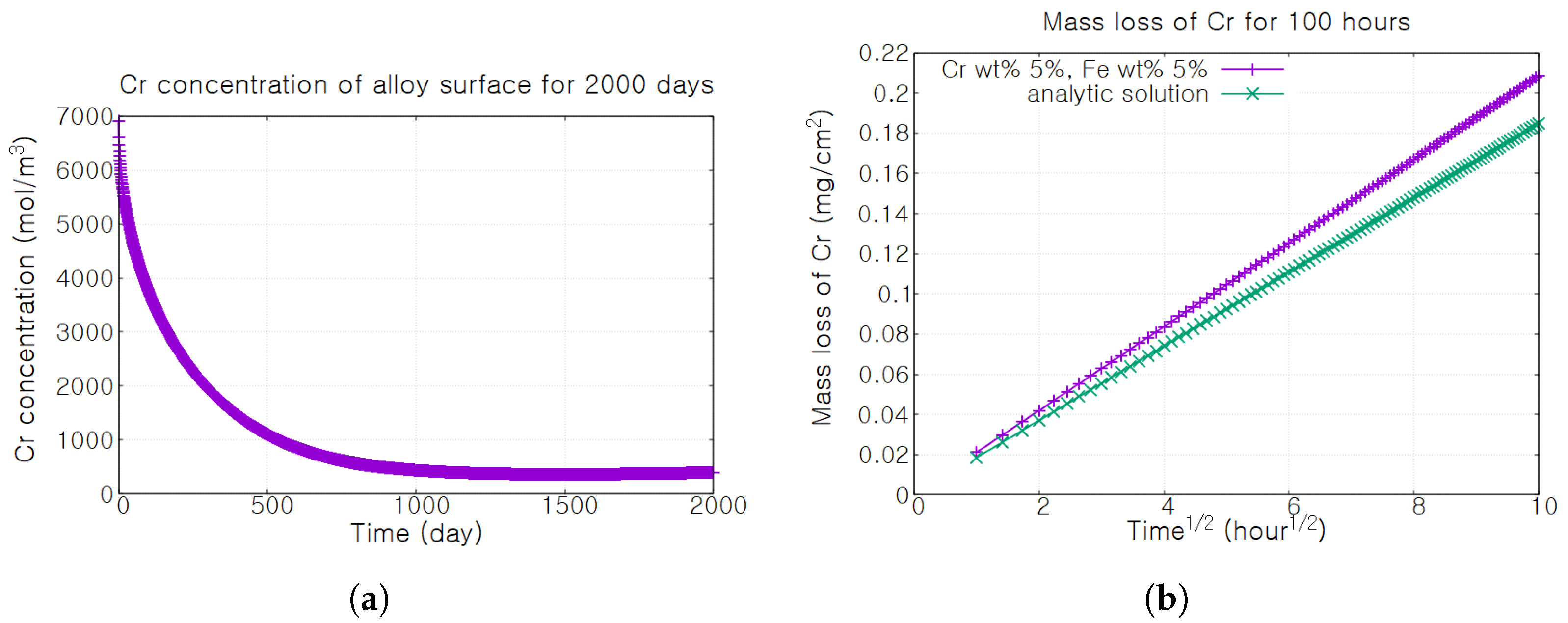
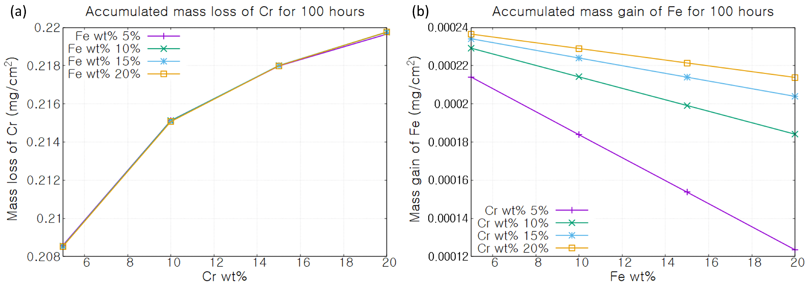
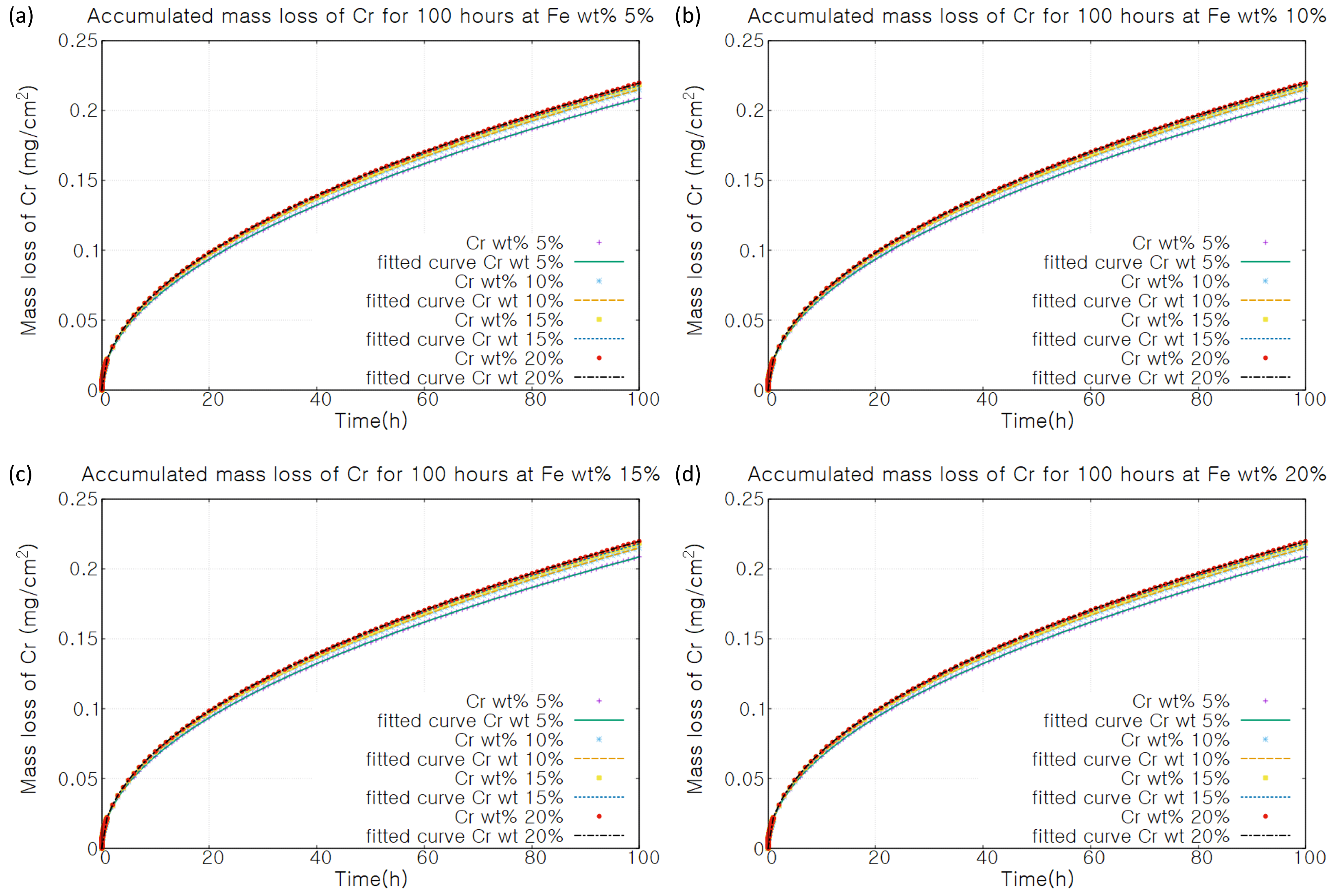
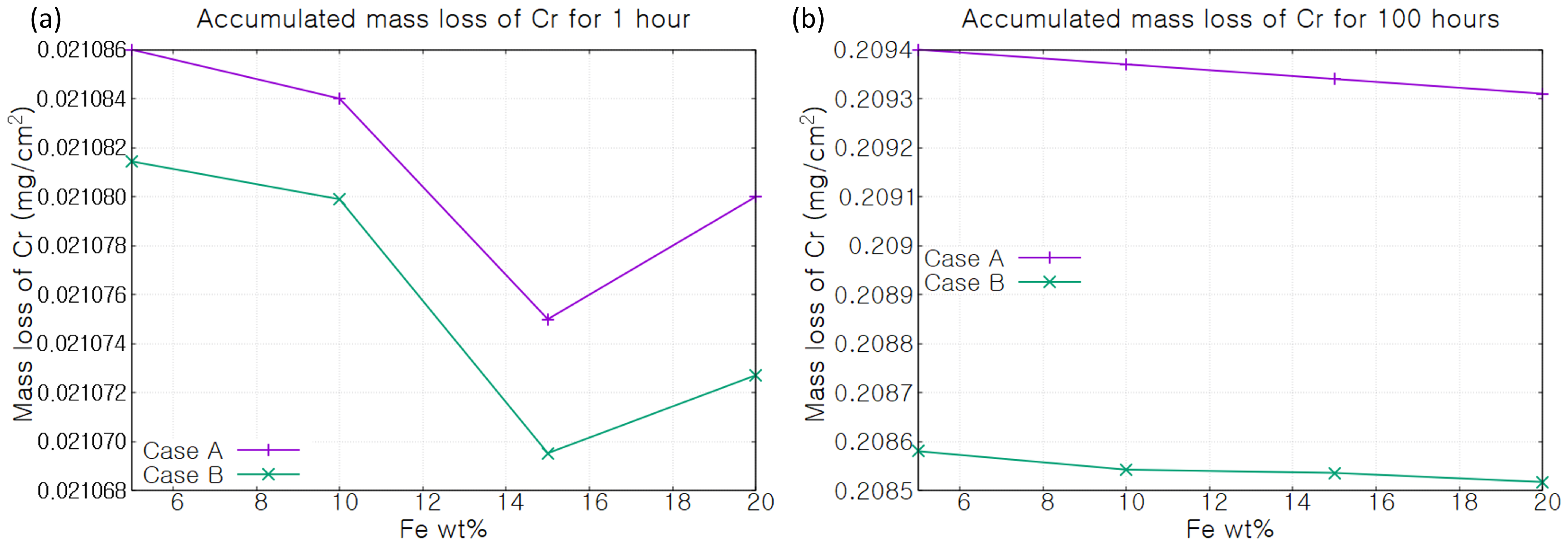
In the model, the temperature of the molten salt is 1023.15 K. The design temperature of the Molten Salt Reactor Experiment is 1300 F ; therefore, we set a higher temperature to be conservative. The viscosity of molten salt is 0.01   Pa · s . The diffusivity of Cr in the alloy is 4.53 × 10 5   μ m 2 / s 1 , considering grain boundary diffusion [30]. The backward differentiation formula (BDF) method is used for the time integration. The time step length from 0 to 10 s is 0.1   s , from 10 s to 3600 s is 10 s and from 3600 s to 100 h is 1 h .
The initial concentrations and properties of the various species are shown in Table 4. The initial concentration of the molten salt is the concentration of the eutectic FLiNaK salt (46.5%LiF-11.5%NaF-42%KF). The initial concentration of HF is set to 100 ppm to conservatively calculate the concentration after purification [35]. The initial concentration and reference concentration of the alloy elements ( Cr 2 + , Cr 3 + , Fe 2 + , Fe 3 + , Ni 2 + ) are from the Redox potential in Figure 8 of [15]. The reference concentration of F is 1000 mol/ m 3 . The reference concentration of HF(g) and H 2 ( g ) is the concentration of ideal gas at 1 mol, 1 atm, 1023.15   K .
The reference properties for each reaction are shown in Table 5. The reference equilibrium potentials for each reaction are calculated using the redox potential in Figure 8 of [15] at 1023.15   K . The reference equilibrium potential of the HF(g) reduction reaction is calculated using the standard Gibbs free energy change of each reactant. The reference exchange current density of Cr and Fe are measured experimentally [36], but the reference exchange current density of Ni is not available in the FLiNaK molten salt; hence, the reference exchange current density of Cr is used. The reference exchange current density of the halogen elements ( Li + , Na + , K + ) are used as the default values in COMSOL because the halogen oxidation reactions are inhibited such that no reaction occurred. The reference exchange current density of the HF reaction is not found; hence, the reference exchange current density of Fe, which is the larger value of Cr and Fe, is used. The anodic transfer coefficient for Cr and Fe are taken from experiments [36], and the default values for the rest of the reactions are taken from COMSOL.
We performed sensitivity analysis for 100 h to check the effect of assumed parameters i 0 , Ni r e f , i 0 , HF r e f , α a , Ni , and α a , HF . As shown in Table 6, the assumed parameters increase and decrease by 50%, and the mass loss of Cr decreases by 0.00001∼0.00002 m g /cm2, which is marginal. As a result, the sensitivity of the assumed parameters to the simulation results is not considered to be high.

3. Results

We begin by verifying our model against an analytical solution. We compare mass loss from a Cr wt% 5%, Fe wt% 5% alloy exposed to FLiNaK at 1023.15 K to the analytic solution [30,37]:
Δ M Cr = 2 ( c 0 c surf ) ρ alloy D Cr t π ,
where Δ M Cr is the mass loss per unit area at some time t, c 0 is the initial mass fraction of Cr in the alloy, ρ alloy is the density of the alloy, D Cr is the diffusivity of Cr in the alloy, and c surf is the mass fraction of Cr at the surface of the material in the surface stable state when no further mass loss is occurring. The simulation was performed for 2000 days and both the mass loss and the surface concentration of Cr were predicted over time.
The progression of the corrosion is clear from the Cr concentration at the surface over time, as shown in Figure 3a. There is rapid Cr depletion at first, but it slows with time. After 1500 days, there is little corrosion progression and at 2000 days, the surface Cr concentration reaches 398.51 mol/ m 3 , or a mass fraction of 0.002878; we used this value as the steady state c surf in the analytical model. ρ alloy is assumed to 8.7   g / cm 3 , which is the Ni–5Cr alloy density [30]. The Cr mass loss by the surface reaction-diffusion-coupled simulation is visualized in Figure 3b along with the analytical prediction by Equation (15). The mass loss of Cr with simulation is 13% larger than the analytic solution on average. The root mean square error between two curves is 0.01699   m g /cm2, indicating reasonable accuracy.
Having verified the performance of our model, we apply it to quantify the impact of the initial alloying element concentrations on the corrosion by molten FLiNaK at 1023.15 K. We vary the initial weight percentages of Cr and Fe from 5% to 20% in 5% increments and simulate the mass change after 1 h and 100 h. To determine whether the behavior of the corrosion during the initial transient period is different from the behavior after the transient, the corrosion behavior after 1 h is evaluated and shown in Figure 4, and the corrosion behavior after 100 h is evaluated and shown in Figure 5. The mass loss for Cr and the mass gain for Fe after 1 h are shown in Figure 4, and the mass loss for Cr and the mass gain for Fe after 100 h are shown in Figure 5. Our results show that mass loss of Cr increases slightly with the weight percent of Cr and is fairly insensitive to the weight percent of Fe. The mass gain of Fe decreases with the increase in weight percent of Fe, but increases with the increase in weight percent of Cr.
Among the corrosion-resistant metals, alloy 800H is a Ni–Fe–Cr alloy, like the material in our simulation model. Therefore, we performed simulation for 500 h with an alloy composition of 35Ni–40Fe–25Cr. The Cr mass change of the 35Ni–40Fe–25Cr condition is 0.49364   m g /cm2. In Table 1 of the corrosion experiment reference [38], Olson’s experiment results [39] for alloy 800H and 500 h are 0.15   m g /cm2 to 51.4   m g /cm2. Olson’s experimental data vary depending on the type of container and whether the salt is purified or not, but our result is within the range of Olson’s experimental data. Therefore, we considered it to be quantitatively consistent.

4. Discussion

We fitted the mass loss of Cr for different wt% Cr and Fe using the expression
Δ M Cr a t b + c t d + e t f
where a, c, and e are the fitting coefficients and b, d, and f are the fitting exponents. Δ M Cr has units of mg/cm2 and the time t has units of hours. The coefficients of Equation (16) for different Cr and Fe wt% obtained via least mean square fitting are shown in Table 7. All of the fits, visualized in Figure 6, are very accurate, with errors less than 0.0004036 mg/cm2.
To observe the effect of Cr depletion on mass loss, the concentration of the surface Cr is fixed at 5% and we simulate the corrosion behavior for two cases:
  • Case A: Cr concentration is fixed within the material.
  • Case B: Cr depletion takes place due to corrosion and Cr atoms diffuse within the material.
As shown in Figure 7, after 1 h, the Cr mass loss for Case A is 0.025% larger than that for Case B on average. After 100 h, the Cr mass loss of Case A is 0.387% larger than Case B on average. The effect of Fe concentration on the amount of Cr corrosion was relatively insignificant. As shown in Figure 8, the average Cr concentration over the surface decreased by 8.9% over 100 h from the start of corrosion, while the effect of Fe concentration in the material was not noticeable.

5. Conclusions and Future Works

We developed a corrosion simulation model that couples surface reaction and diffusion processes under molten salt conditions. The model simultaneously analyzes multiple phenomena, including diffusion, mass transfer, and electrochemical reactions. This model was used to predict the corrosion behavior of Ni–Cr–Fe alloys in F–Li–Na–K molten salt, both with and without considering the diffusion of Cr within the material. The results were compared to analytical solutions. The reduction reaction assumed that gaseous HF accepts electrons and decomposes into hydrogen gas and F ions. When Cr diffusion was accounted for, it resulted in Cr depletion at the surface, which reduced the corrosion rate compared to the case where diffusion was not considered. As the Cr concentration in the alloy increased, the mass loss due to Cr corrosion increased, while the mass loss from Fe corrosion decreased. Conversely, increasing the Fe concentration led to greater mass loss from Fe corrosion, but the Cr corrosion remained unaffected. This study did not consider any microstructural inhomogeneities other than the Cr concentration gradient, and we believe that it is necessary to reflect defects such as grain boundaries for a more realistic simulation. In particular, the grain boundary is an important pathway for Cr depletion, which is known to be an important corrosion mechanism, and the simulation of corrosion phenomena, including grain boundary diffusion and grain-boundary–solute interaction, is considered an important future work. Also, from a system perspective, to simulate a more realistic molten salt reactor environment, we believe it is essential to incorporate the effects of molten salt flow and temperature gradients in both the material and the molten salt.

Author Contributions

Conceptualization, K.C. and M.R.T.; methodology, K.C. and M.C.; software, M.C.; validation, M.C. and K.C.; formal analysis, M.C.; investigation, M.C.; resources, M.C.; data curation, M.C.; writing—original draft preparation, M.C.; writing—review and editing, K.C. and M.R.T.; visualization, M.C.; supervision K.C.; project administration, K.C.; funding acquisition. K.C. All authors have read and agreed to the published version of the manuscript.

Funding

This work was supported by the Korea Institute of Energy Technology Evaluation and Planning (KETEP) grant funded by the Korea government (MOTIE) (No. 20224000000550, Training of simulation experts for the development of structural materials for molten salt reactors and RS-2024-00349003). This study was also supported by the National R&D Program through the National Research Foundation of Korea (NRF) funded by the Ministry of Science and ICT (RS-2023-00229215) of the Republic of Korea.

Data Availability Statement

The original contributions presented in the study are included in the article, further inquiries can be directed to the corresponding author.

Conflicts of Interest

The authors declare no conflict of interest.

References

  1. Lane, J.A.; MacPherson, H.G.; Maslan, F. Fluid Fuel Reactors: Molten Salt Reactors, Aqueous Homogeneous Reactors, Fluoride Reactors, Chloride Reactors, Liquid Metal Reactors and Why Liquid Fission; Addison-Wesley Publishing Co., Ltd.: London, UK, 1958. [Google Scholar]
  2. Beneš, O.; Souček, P. 6—Molten salt reactor fuels. In Advances in Nuclear Fuel Chemistry; Piro, M.H., Ed.; Woodhead Publishing Series in Energy; Woodhead Publishing: Sawston, UK, 2020; pp. 249–271. [Google Scholar] [CrossRef]
  3. Serp, J.; Allibert, M.; Beneš, O.; Delpech, S.; Feynberg, O.; Ghetta, V.; Heuer, D.; Holcomb, D.; Ignatiev, V.; Kloosterman, J.L.; et al. The molten salt reactor (MSR) in generation IV: Overview and perspectives. Prog. Nucl. Energy 2014, 77, 308–319. [Google Scholar] [CrossRef]
  4. Fredrickson, G.L.; Cao, G.; Gakhar, R.; Yoo, T.S. Molten Salt Reactor Salt Processing—Technology Status; Idaho National Laboratory (INL): Idaho Falls, ID, USA, 2018. [CrossRef]
  5. Robertson, R.C. MSRE Design & Operations Report Part 1 Description of Reactor Design; Oak Ridge National Laboratory (ORNL): Oak Ridge, TN, USA, 1965. [CrossRef]
  6. Rosenthal, M.; Kasten, P.; Briggs, R. Molten-salt reactors—History, status, and potential. Nucl. Appl. Technol. 1970, 8, 107–117. [Google Scholar] [CrossRef]
  7. Ho, M.; Yeoh, G.; Braoudakis, G. Molten Salt Reactors, Materials and Processes for Energy: Communicating Current Research and Technological Developments; Formatex Research Center: Norristown, PA, USA, 2013; pp. 761–768. [Google Scholar]
  8. Lantelme, F.; Groult, H. Molten Salts Chemistry: From Lab to Applications; Newnes: Oxford, UK, 2013. [Google Scholar]
  9. Kamei, T.; Hakami, S. Evaluation of implementation of thorium fuel cycle with LWR and MSR. Prog. Nucl. Energy 2011, 53, 820–824. [Google Scholar] [CrossRef]
  10. Elsheikh, B.M. Safety assessment of molten salt reactors in comparison with light water reactors. J. Radiat. Res. Appl. Sci. 2013, 6, 63–70. [Google Scholar] [CrossRef]
  11. Guo, S.; Zhang, J.; Wu, W.; Zhou, W. Corrosion in the molten fluoride and chloride salts and materials development for nuclear applications. Prog. Mater. Sci. 2018, 97, 448–487. [Google Scholar] [CrossRef]
  12. Ignatiev, V.; Surenkov, A. 5-Corrosion phenomena induced by molten salts in Generation IV nuclear reactors. In Structural Materials for Generation IV Nuclear Reactors; Yvon, P., Ed.; Woodhead Publishing: Sawston, UK, 2017; pp. 153–189. [Google Scholar] [CrossRef]
  13. Yoshioka, R.; Kinoshita, M.; Scott, I. 7—Materials. In Molten Salt Reactors and Thorium Energy; Dolan, T.J., Ed.; Woodhead Publishing: Sawston, UK, 2017; pp. 189–207. [Google Scholar] [CrossRef]
  14. Niketan, S.; Patel, V.P.; Boča, M. High-Temperature Corrosion Behavior of Superalloys in Molten Salts—A Review. Crit. Rev. Solid State Mater. Sci. 2017, 42, 83–97. [Google Scholar] [CrossRef]
  15. Zhang, J.; Forsberg, C.W.; Simpson, M.F.; Guo, S.; Lam, S.T.; Scarlat, R.O.; Carotti, F.; Chan, K.J.; Singh, P.M.; Doniger, W.; et al. Redox potential control in molten salt systems for corrosion mitigation. Corros. Sci. 2018, 144, 44–53. [Google Scholar] [CrossRef]
  16. Khanna, A.S. Introduction to High Temperature Oxidation and Corrosion; ASM International: Almere, The Netherlands, 2002. [Google Scholar]
  17. MacPherson, H. Development of materials and systems for the molten-salt reactor concept. React. Technol. 1972, 15, 136–155. [Google Scholar]
  18. Abu-warda, N.; García-Rodríguez, S.; Torres, B.; Utrilla, M.V.; Rams, J. Effect of Molten Salts Composition on the Corrosion Behavior of Additively Manufactured 316L Stainless Steel for Concentrating Solar Power. Metals 2024, 14, 639. [Google Scholar] [CrossRef]
  19. Kanjanaprayut, N.; Siripongsakul, T.; Promdirek, P. Intergranular Corrosion Analysis of Austenitic Stainless Steels in Molten Nitrate Salt Using Electrochemical Characterization. Metals 2024, 14, 106. [Google Scholar] [CrossRef]
  20. Fernández, A.; Galleguillos, H.; Fuentealba, E.; Pérez, F. Corrosion of stainless steels and low-Cr steel in molten Ca(NO3)2–NaNO3–KNO3 eutectic salt for direct energy storage in CSP plants. Sol. Energy Mater. Sol. Cells 2015, 141, 7–13. [Google Scholar] [CrossRef]
  21. Soleimani Dorcheh, A.; Durham, R.N.; Galetz, M.C. Corrosion behavior of stainless and low-chromium steels and IN625 in molten nitrate salts at 600 °C. Sol. Energy Mater. Sol. Cells 2016, 144, 109–116. [Google Scholar] [CrossRef]
  22. Sun, H.; Wang, J.; Li, Z.; Zhang, P.; Su, X. Corrosion behavior of 316SS and Ni-based alloys in a ternary NaCl-KCl-MgCl2 molten salt. Sol. Energy 2018, 171, 320–329. [Google Scholar] [CrossRef]
  23. Wang, J.-W.; Zhang, C.-Z.; Li, Z.-H.; Zhou, H.-X.; He, J.-X.; Yu, J.-C. Corrosion behavior of nickel-based superalloys in thermal storage medium of molten eutectic NaCl-MgCl2 in atmosphere. Sol. Energy Mater. Sol. Cells 2017, 164, 146–155. [Google Scholar] [CrossRef]
  24. Muránsky, O.; Yang, C.; Zhu, H.; Karatchevtseva, I.; Sláma, P.; Nový, Z.; Edwards, L. Molten salt corrosion of Ni-Mo-Cr candidate structural materials for Molten Salt Reactor (MSR) systems. Corros. Sci. 2019, 159, 108087. [Google Scholar] [CrossRef]
  25. Delpech, S.; Carrière, C.; Chmakoff, A.; Martinelli, L.; Rodrigues, D.; Cannes, C. Corrosion Mitigation in Molten Salt Environments. Materials 2024, 17, 581. [Google Scholar] [CrossRef]
  26. Mcmurray, J.W.; Besmann, T.M.; Ard, J.; FItzpatrick, B.; Piro, M.; Jerden, J.; Williamson, M.; Collins, B.S.; Betzler, B.R.; Qualls, A.L. Multi-Physics Simulations for Molten Salt Reactor Evaluation: Chemistry Modeling and Database Development; Oak Ridge National Laboratory (ORNL): Oak Ridge, TN, USA, 2018. [CrossRef]
  27. MaeHyun, C.; Hyeong-Jun, J.; Jungshin, K.; Kunok, C. Development of Numerical Analysis Model for New Magnesium Electrolysis Process Using COMSOL. Korean J. Met. Mater. 2023, 61, 625–631. [Google Scholar] [CrossRef]
  28. Wang, W.; Guan, B.; Wei, X.; Lu, J.; Ding, J. Cellular automata simulation on the corrosion behavior of Ni-base alloy in chloride molten salt. Sol. Energy Mater. Sol. Cells 2019, 203, 110170. [Google Scholar] [CrossRef]
  29. Li, X.; Xu, T.; Liu, M.; Song, Y.; Zuo, Y.; Tang, Z.; Yan, L.; Wang, J. Thermodynamic and kinetic corrosion behavior of alloys in molten MgCl2–NaCl eutectic: FPMD simulations and electrochemical technologies. Sol. Energy Mater. Sol. Cells 2022, 238, 111624. [Google Scholar] [CrossRef]
  30. Vivek Bhave, C.; Zheng, G.; Sridharan, K.; Schwen, D.; Tonks, M.R. An electrochemical mesoscale tool for modeling the corrosion of structural alloys by molten salt. J. Nucl. Mater. 2023, 574, 154147. [Google Scholar] [CrossRef]
  31. Feng, J.; Gao, J.; Mao, L.; Bedell, R.; Liu, E. Modeling the Impact of Grain Size on Corrosion Behavior of Ni-Based Alloys in Molten Chloride Salt via Cellular Automata. Metals 2024, 14, 931. [Google Scholar] [CrossRef]
  32. Kane, R.D. Molten Salt Corrosion. In Corrosion: Fundamentals, Testing, and Protection; ASM International: Almere, The Netherlands, 2003. [Google Scholar] [CrossRef]
  33. Was, G.; Kruger, R. A thermodynamic and kinetic basis for understanding chromium depletion in Ni-Cr-Fe alloys. Acta Metall. 1985, 33, 841–854. [Google Scholar] [CrossRef]
  34. Einstein, A. Über die von der molekularkinetischen Theorie der Wärme geforderte Bewegung von in ruhenden Flüssigkeiten suspendierten Teilchen. Ann. Phys. 1905, 4, 549–560. [Google Scholar] [CrossRef]
  35. Zuo, Y.; Song, Y.L.; Tang, R.; Qian, Y. A novel purification method for fluoride or chloride molten salts based on the redox of hydrogen on a nickel electrode. RSC Adv. 2021, 11, 35069–35076. [Google Scholar] [CrossRef] [PubMed]
  36. Wu, W.; Guo, S.; Zhang, J. Exchange Current Densities and Charge-Transfer Coefficients of Chromium and Iron Dissolution in Molten LiF-NaF-KF Eutectic. J. Electrochem. Soc. 2017, 164, C840. [Google Scholar] [CrossRef]
  37. Zheng, G. Corrosion Behavior of Alloys in Molten Fluoride Salts. Ph.D. Thesis, University of Wisconsin, Madison, WI, USA, 2015. [Google Scholar]
  38. Raiman, S.S.; Lee, S. Aggregation and data analysis of corrosion studies in molten chloride and fluoride salts. J. Nucl. Mater. 2018, 511, 523–535. [Google Scholar] [CrossRef]
  39. Olson, L.C.; Ambrosek, J.W.; Sridharan, K.; Anderson, M.H.; Allen, T.R. Materials corrosion in molten LiF–NaF–KF salt. J. Fluor. Chem. 2009, 130, 67–73. [Google Scholar] [CrossRef]
Figure 1. Schematic geometry of the model. The blue region is the molten salt (electrolyte), the grey region is the alloy (electrode), and the red region is the alloy surface where the reactions occur.
Metals 14 01088 g001
Figure 2. The mesh used for our simulations, where the system area is 10 4   m 2 and the element size is 5 × 10 4   m .
Metals 14 01088 g002
Figure 3. Simulation of corrosion of a 5% Cr, 5% Fe by weight alloy exposed to FLiNaK at 1023.15 K. The surface concentration of Cr over time is shown in (a). The mass loss over time from the simulation and from Equation (15) are shown in (b).
Metals 14 01088 g003
Figure 4. Mass loss for 1 h (a) mass loss of Cr by Cr wt%, (b) mass gain of Fe by Fe wt%.
Metals 14 01088 g004
Figure 5. Mass loss for 100 h (a) mass loss of Cr by Cr wt%, (b) mass gain of Fe by Fe wt%.
Metals 14 01088 g005
Figure 6. Fits of the mass loss of Cr versus time (a) 5 wt% Fe; (b) 10 wt% Fe; (c) 15 wt% Fe; (d) 20 wt% Fe. Maximum error of the fits is 0.0004036 mg/cm2.
Metals 14 01088 g006
Figure 7. Mass loss of Cr for 1 h (a) and 100 h (b) at 5% Cr weight percent.
Metals 14 01088 g007
Figure 8. Surface concentration of Cr with respect to time at 5% Cr weight percent.
Metals 14 01088 g008
Table 1. Comparison between previous works [28,29,30] and current work.
AlloyMolten SaltMicrostructureSurface Reaction
Wang et al. [28]625NaCl–MgCl2–CaCl2N/AStochastic approach
Li et al. [29]Ni-Cr-Fe-Mn-CoNaCl–MgCl2N/ABerzins-Delahay
Bhave et al. [30]Ni-CrFLiBeGrain BoundarySimplified Butler-Volmer
Feng et al. [31]625ChlorideGrain BoundaryStochastic approach
Current workNi-Cr-FeFLiNaKN/AButler-Volmer
Table 2. Reactions occurring on the electrode surface.
Oxidation ReactionReduction Reaction
Cr ( s ) Cr 2 + + 2 e Li + + e Li ( s )
Cr ( s ) Cr 3 + + 3 e Na + + e Na ( s )
Fe ( s ) Fe 2 + + 2 e K + + e K ( s )
Fe ( s ) Fe 3 + + 3 e HF ( g ) + e 1 2 H 2 ( g ) + F
Ni ( s ) Ni 2 + + 2 e
Table 3. Example of the stoichiometry coefficient and the number of electrons participating.
o x | v o x | S o x + n e r e d v r e d S r e d
Cr ( s ) Cr 2 + + 2 e
n = 2
S o x = Cr 2 + v Cr 2 + = 1
S r e d = Cr ( s ) v Cr ( s ) = 1
Table 4. Species initial conditions and properties, including the initial concentration c j 0 and the reference concentration in the molten salt and alloy used in Equations (10) and (12), and the radius r j used in Equation (5).
Species j c j 0 (mol/m3) c j ref (mol/m3) r j (Å)
F 59,674.2610001.33
Li + 38,342.3938,342.390.76
Na + 5861.1985861.1981.02
K + 15,470.6815,470.681.38
Cr 2 + 10 3 10 3 0.87
Cr 3 + 10 3 10 3 0.755
Fe 2 + 10 3 10 3 0.75
Fe 3 + 10 3 10 3 0.69
Ni 2 + 10 3 10 3 0.70
HF(g)5.967411.911.55
H 2 ( g ) 10 3 11.910.1
Cr a l l o y 138,461.5385138,461.5385-
Table 5. Reaction properties, including the reference equilibrium potential E e q , j r e f used in Equation (12), the reference exchange current density i 0 , j r e f used in Equation (9), and the anodic transfer coefficient α a , j used in Equation (9).
ReactionSpecies j E eq , j ref (V) i 0 , j ref (mA/cm2) α a , j
Cr ( s ) Cr 2 + + 2 e Cr 2 + −3.90.880.22
Cr ( s ) Cr 3 + + 3 e Cr 3 + −3.550.880.22
Fe ( s ) Fe 2 + + 2 e Fe 2 + −3.56.150.11
Fe ( s ) Fe 3 + + 3 e Fe 3 + −3.16.150.11
Ni ( s ) Ni 2 + + 2 e Ni 2 + −3.050.880.22
Li + + e Li ( s ) Li + −5.450.050.5
Na + + e Na ( s ) Na + −5.10.050.5
K + + e K ( s ) K + −4.90.050.5
HF ( g ) + e 1 2 H 2 ( g ) + F HF(g)−2.896.150.5
Table 6. Sensitivity analysis results for 100 h of assumed parameters i 0 , Ni r e f , i 0 , HF r e f , α a , Ni , α a , HF .
i 0 , Ni ref (mA/cm2) α a , Ni Mass Loss of Cr (mg/cm2) i 0 , HF ref (mA/cm2) α a , HF Mass Loss of Cr (mg/cm2)
0.440.110.208563.0750.250.20857
0.880.220.208586.150.50.20858
1.320.330.208569.2250.750.20857
Table 7. Coefficients of the fitting curve by alloy compositions.
Cr/Fe wt%abcdef
5%/5%−0.3053260.2251550.2919360.2174240.03436780.451575
5%/10%−0.3055210.2279010.2917630.2200850.03473560.450973
5%/15%−0.3051280.2250010.2921240.2174760.03397320.452563
5%/20%−0.3052430.2251540.2920160.2175010.03419760.452018
10%/5%−0.3043310.2152280.2930860.2081620.03283370.457936
10%/10%−0.304190.2153450.2932230.2084080.03255750.458842
10%/15%−0.3050040.2214130.2924550.2138310.03413660.454917
10%/20%−0.3050470.2222660.2924130.2146580.03422470.454917
15%/5%−0.3044880.2148790.2929530.2076150.03340260.457576
15%/10%−0.3045170.2159660.2929290.2086820.03346170.457616
15%/15%−0.3048120.2174290.2926490.2098750.03403120.456204
15%/20%−0.3046810.2170780.2927750.2096520.03377590.456869
20%/5%−0.3021050.1909260.2952580.1858820.02887440.470715
20%/10%−0.3042360.2129260.2932030.2058230.03307260.45927
20%/15%−0.3037690.2090210.2936490.2023660.03215520.451467
20%/20%−0.3040030.2115950.2934270.2047240.03261910.460399
Disclaimer/Publisher’s Note: The statements, opinions and data contained in all publications are solely those of the individual author(s) and contributor(s) and not of MDPI and/or the editor(s). MDPI and/or the editor(s) disclaim responsibility for any injury to people or property resulting from any ideas, methods, instructions or products referred to in the content.

