3.1. Flow Stress Modeling of AISI-1045 Steel Using an ANN with Back-Propagation Algorithm
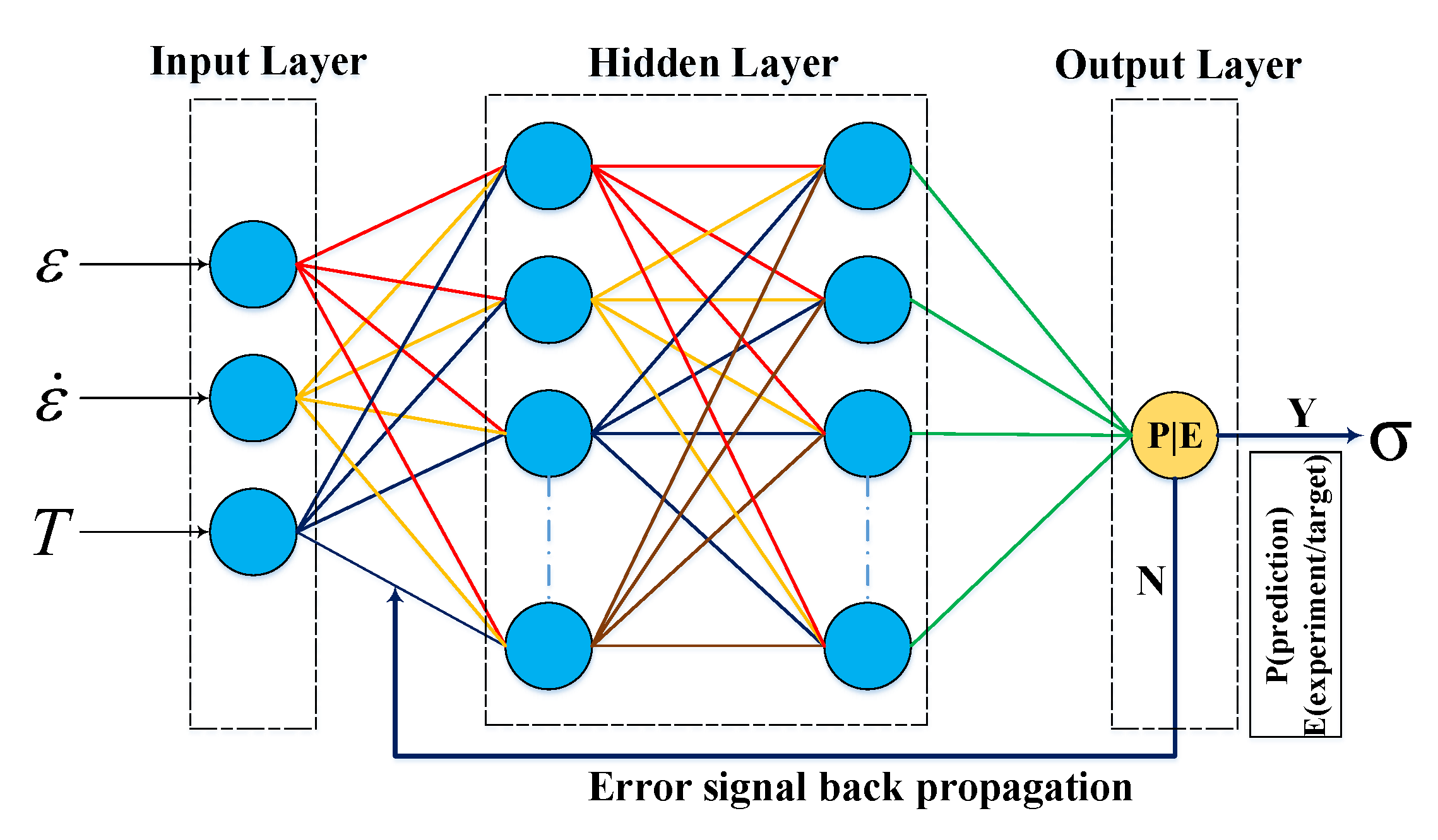
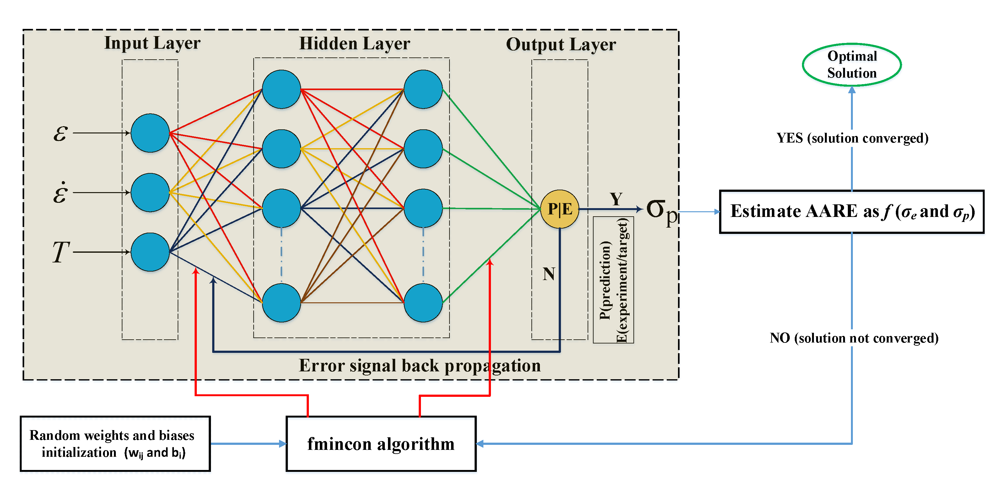
In this research work, a multi-layer feed forward ANN model with supervised learning procedure, BP algorithm for training, was employed to construct the functional relationship among input and output variables for predicting flow stress at hot working conditions as shown in
Figure 3. As can be seen in
Figure 3, there were three input variables: strain (
), strain rate (
), and deformation temperature (
T), and one output variable, stress (
), in the neural network design. The network training began with initialization of random weights and biases, and then the weight was adjusted based on the prediction error between computed and experimental observations using BP learning algorithm. In detail, the process involved two steps: forward and backward pass. At first, the model inputs were fed into the network with casual weights and arrived at the output layer with the approximate solution. Thereafter, in a backward pass, the output from the forward pass was compared against the real data, and then the weights and biases were altered iteratively to minimize the mean square error (MSE) (Equation (1)) with the help of BP learning algorithm and the process was continuous for each input–output pair throughout the modeling process [
36].
In Equation (1), n is the total number of samples used for training the network. After training the network with each input–output pair, the trained network model c ouldbe tested using unknown input–output sets for evaluating the performance of the proposed network model.
It is obvious that there is no proper ground rule or fixed procedures for selecting initial random weights, the size of training data set, total number of neurons in the hidden layer, learning algorithm (weight adjustment) and transfer functions in order to construct the ANN-BP model. In this research work, from literature survey, the detailed procedures to adopt the hidden layer with the optimum number of neurons, number of samples, learning algorithms and activation functions are presented. Carpenter et al. [
37] suggested that in the hidden layer, number of neurons in terms of minimum counts can be explained using the following expressions:
whereas, in Equation (2), HN and IN are number of neurons in the hidden layer and number of variables in the input layer, respectively. Accordingly, for this research work, in the hidden layer, number of neurons varied from 2 to 30 to confirm the capability of Equation (2).
Further, for training the neural network model, a minimum number of required sample data are estimated as follows [
38,
39]:
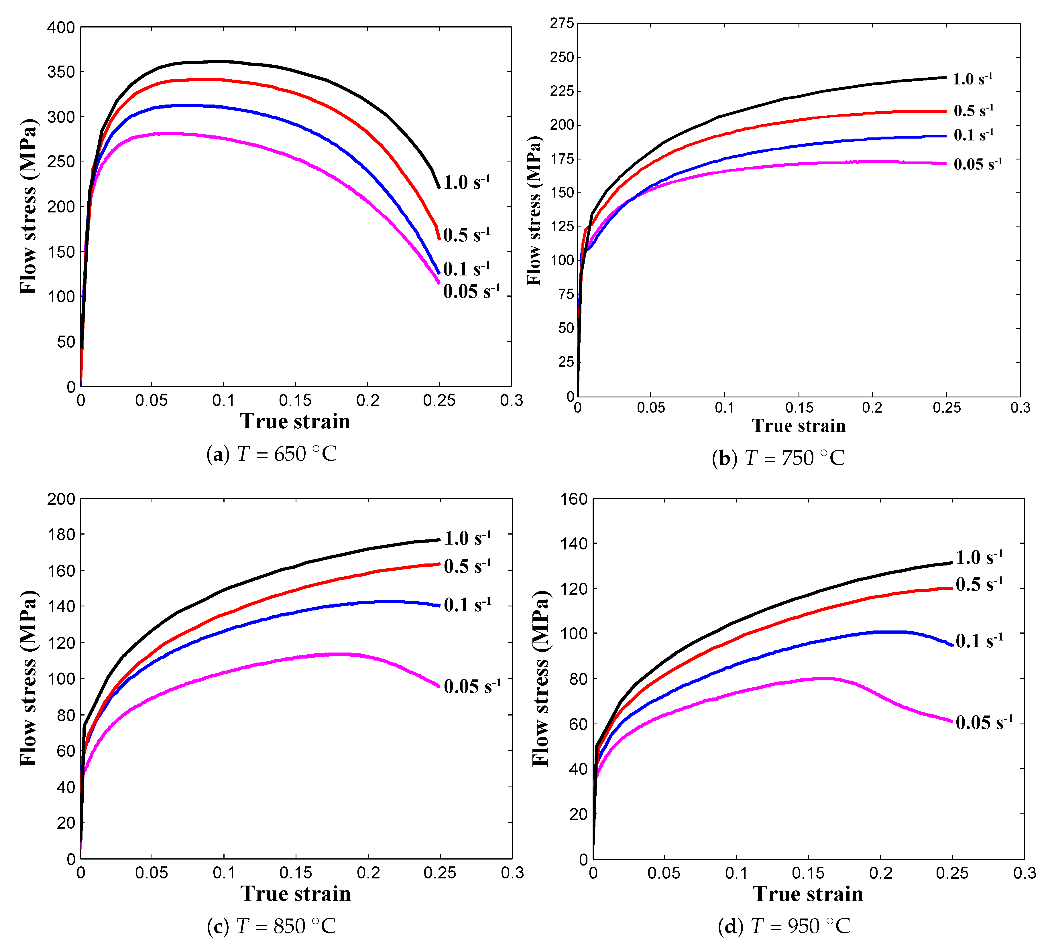
In Equation (3), NO and NT are number of variables in the output layer and number of training data, respectively. It is important to mention here that sample counts are essential in order to effectively train the network as it has a huge influence on network generations for producing close predictions. Using Equation (3), the minimum number of samples for one test condition were estimated as 21 and for all conditions, the total number of samples were calculated as 336. In addition, for improving performance of network generations and also for capturing a wide range of variations, the sample counts were increased from 336 to 384 and kept constant throughout the modeling process. The significant logic behind 384 data selection: in this research work, 16 sets of test conditions were investigated thorough the real time experiments for capturing material deformation behavior. From SS curves as shown in
Figure 1, the plastic range in terms of strain (
) was identified as
to
. Thus, in order to eliminate the inconsistent results from under and over fitting of training data, the data are evenly considered with the strain increment of
and eventually, 24 samples were accounted for each test condition to construct the neural network model.
Before the network training process, entire input and output variables are normalized in order to obtain a usable form for the network using Equation (4).
where
X is the measured experimental data,
and
are the minimum and maximum values of chosen actual data such as stress (
), strain (
), strain rate (
), and deformation temperature (
T), respectively, and
is the normalized data. The experimental values are normalized between more than 0 and less than 0.95, because in the end points, the transfer functions showed a slow learning rate behavior while training the network model [
40]. Likewise, data samples (100%) are randomly partitioned into three sets as training set (70%), validation set (15%) and test set (15%) as listed in
Table 2 in order to perform the network training process. Training and validation sets are used for training the network and monitoring the training process, respectively, whereas the test set is used to examine the performance of trained network in untrained samples.
The selection of activation functions also influences the performance of the neural network in terms of capturing the function approximations among input and output variables. For choosing transfer function in the hidden layer, two most widely used functions such as tan–sigmoid (Equation (5)) and log–sigmoid (Equation (6)), are adopted, because from
Figure 1a–d, the variations (
) are noticed to vary continuously but not linearly as changing input variables (
T,
,
). The reason for choosing sigmoid functions is that it always produces an “S” shape output as shown in
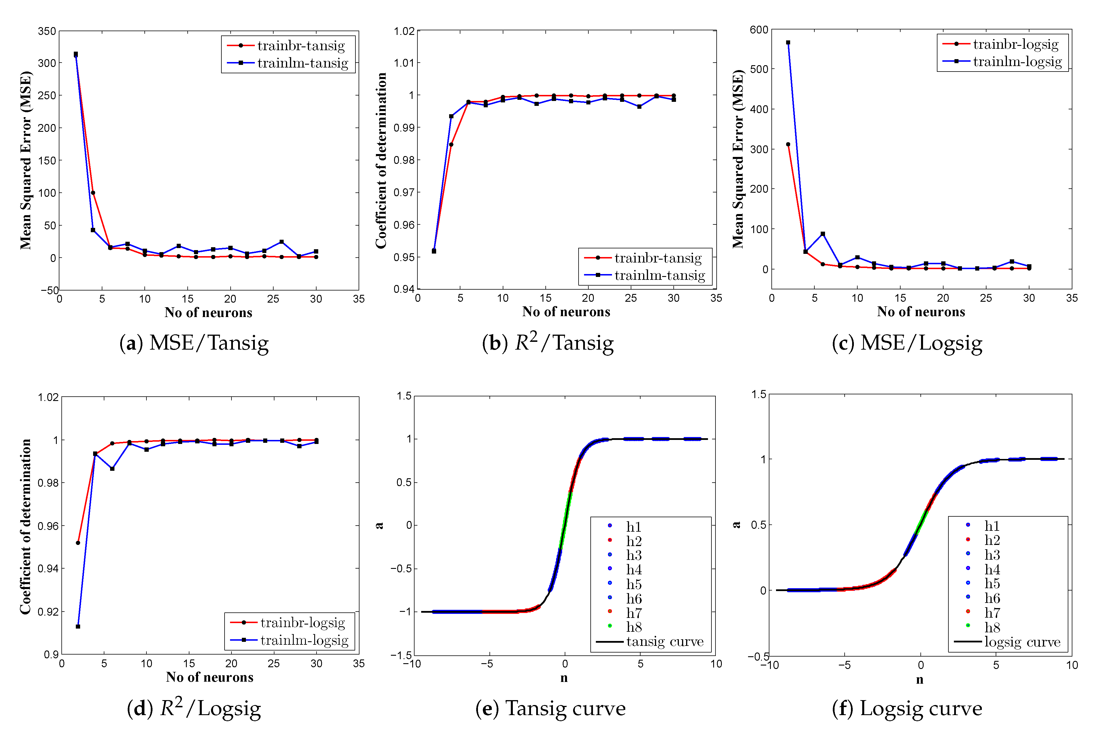
Figure 4e,f; the shape is tends to be linear in the middle and nonlinear towards the boundaries. From
Figure 4e,f, the transfer function, log–sigmoid, was noticed to produce only positive values, which is not suitable if the network expects to return negative values during the training process, whereas tan–sigmoid delivered values from positive to negative, which is suitable in any cases. However, some trail and error calculation procedures were required to select the activation function, in which the network always contributed the optimal solutions. In addition, among the available training functions, trainbr (Bayesian regularization) and trainlm (Levenberg–Marquardt) functions were picked based on their capability to learn to map inputs to outputs within given data-set. For the output layer, the transfer function was directly selected as purelin (linear function) because the problem assumed to be linear in the output layer as the model output was proportional to the total weighted inputs.
Using an ANN-BP model informations summarized in
Table 2, the network models were trained, validated, and tested against the experimental observations. Thereafter, the computed results of MSE and coefficient of determination (
) are plotted against neurons as depicted in
Figure 4a–d.
Figure 4a–d distinctly show that there is little difference between activation functions in terms of MSE and
values. But somehow, there are considerable deviations among the training functions and trainbr function is found to be the best selection for training the network as it displays steady improvement in terms of error decrements along with the highest correlation (
) value. As expected based on Equation (2), from
Figure 4a–d, it is confirmed that the prediction error is significantly higher value up to four neurons. As listed in
Table 3, It is obvious that more number of neurons lead to higher accuracy, but however, after 18 neurons (trainbr), error sums are fluctuating in a random manner. This fluctuation conveys that in order to control over-fitting with unknown points, the size of neurons should be limited to acceptable margin. Therefore, considering the network model complexity, the error differences are inspected closely from 4 to 30 neurons and identified that the predicted results are reasonably accurate when the network contains eight neurons in the hidden layer.
Ultimately, an ANN-BP model consists of one hidden layer with eight neurons, trainbr algorithm as training function, learngdm algorithm as a learning function, and one output layer is chosen for predicting the flow stress at hot working conditions. Moreover, the network model performance also depends on learning parameters, such as the number of training epochs and the performance goal, etc. But in this work, the number of epochs, the learning rate, and the error threshold were fixed to a certain level based on the literature survey as 1000, 0.05 and 1
, respectively. The MSE quantity between actual and predicted data was recorded during network model training and using minimized or converged MSE value, the best models were obtained for both activation functions. Now the trained ANN-BP model should be verified to make a confirmation that the model implementation was done correctly. It is obvious that, in machine learning process, the model performance evaluation and its interpret-ability are the vital procedures for pointing out a solid conclusion about the proposed ANN-BP model. Here, we exploited some helpful procedures such as quantification and visualization methods to comment about the developed flow stress model accuracy in an explicit manner. In addition, there are a few other possible evaluation checks available like examining the proposed model in unknown points, technically called as untrained samples, to monitor the model predictability. These interpretation choices are discussed here in detail, particularly, by both numerical and graphical validations. Moreover, the evaluation techniques presented in this research work is significantly sufficient to confirm the model capability, because the prediction outcomes are always tested against experimental observations. For quantification purpose, three kinds of statistical parameters such as
, average absolute relative error (AARE), and root mean square error (RMSE) are utilized.
explains the prediction strength against experimental observations in terms of a quantity ranging from 0 to 1, whereas AARE is employed to quantify the prediction error at overall test conditions against the experimental data. RMSE is a statistical measure of differences between values predicted by a proposed model and the values actually measured from the experiments [
41].
where
,
,
are the experimental data, the predicted flow stress from an ANN-BP model, and the mean flow stress, respectively, and
n is the total number of data points.
Using Equations (
7) and (
8), the population parameters are computed for each test conditions and summarized in
Table 4. It is clearly seen that both transfer functions in the hidden layer displayed a significantly better outcome. For tansig activation function,
and AARE were estimated as 0.9980 and 1.3348%, respectively, and whereas for logsig activation function,
R2 and AARE were determined as 0.9991 and 1.8059%, respectively. But, in test conditions, 850
C and 950
C, the prediction error was found to be higher, but it was significantly acceptable as the error value was close to 2.2%. Apart from the numerical validation, the graphical validation against the experimental observations was plotted as depicted in
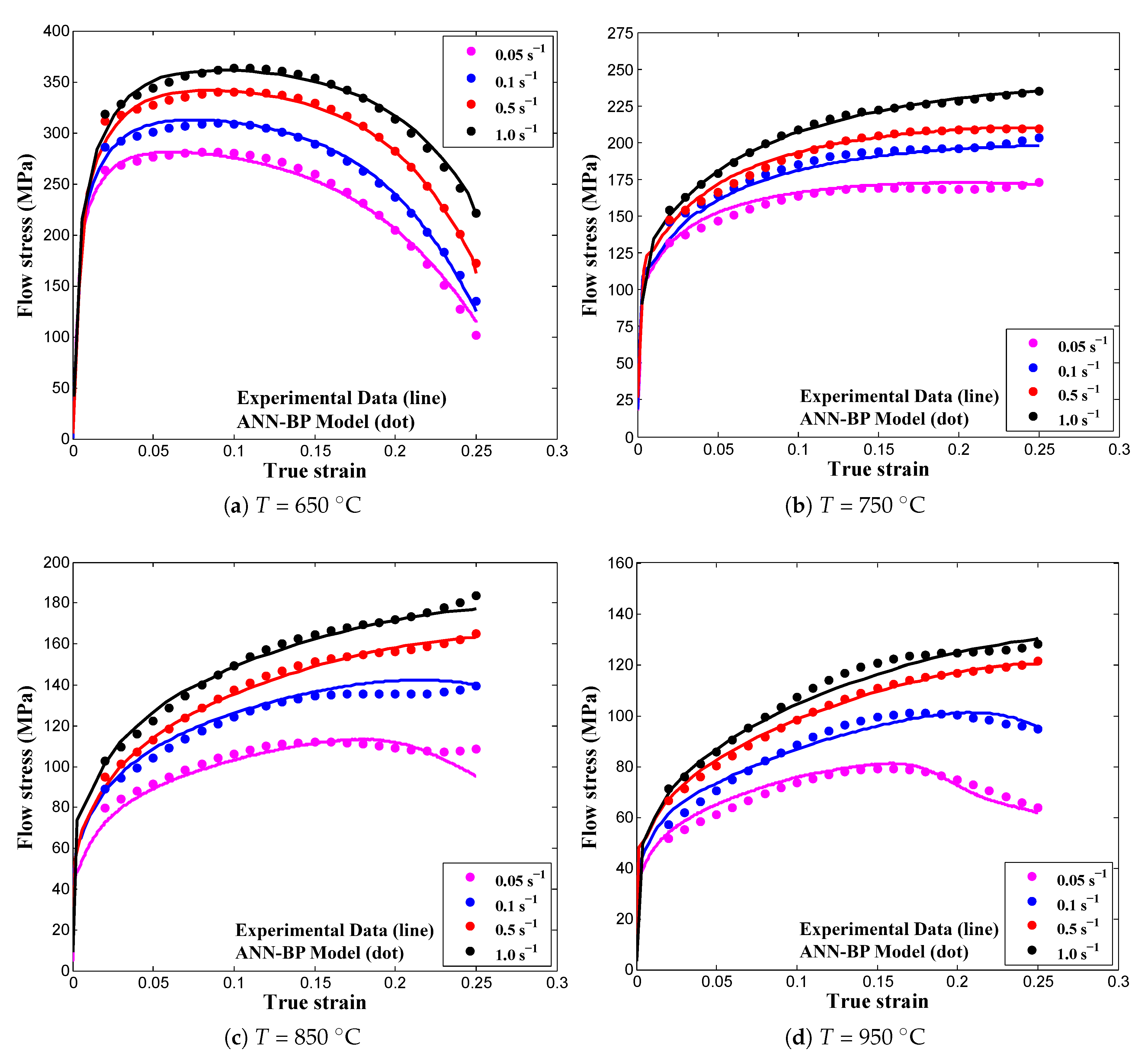
Figure 5 for tansig activation function to prove an ANN-BP model capability.
Figure 5 displays that the model predictions were scattered closer to the experimental data and it confirms that the ANN-BP model can provide accurate representation of material flow behavior under hot deformation conditions. Moreover, the plastic-instability phenomenon also tended to be captured more effectively than that of available traditional flow stress models [
8,
9].
3.2. Optimization Procedures for Obtaining the Best Trained ANN-BP Model
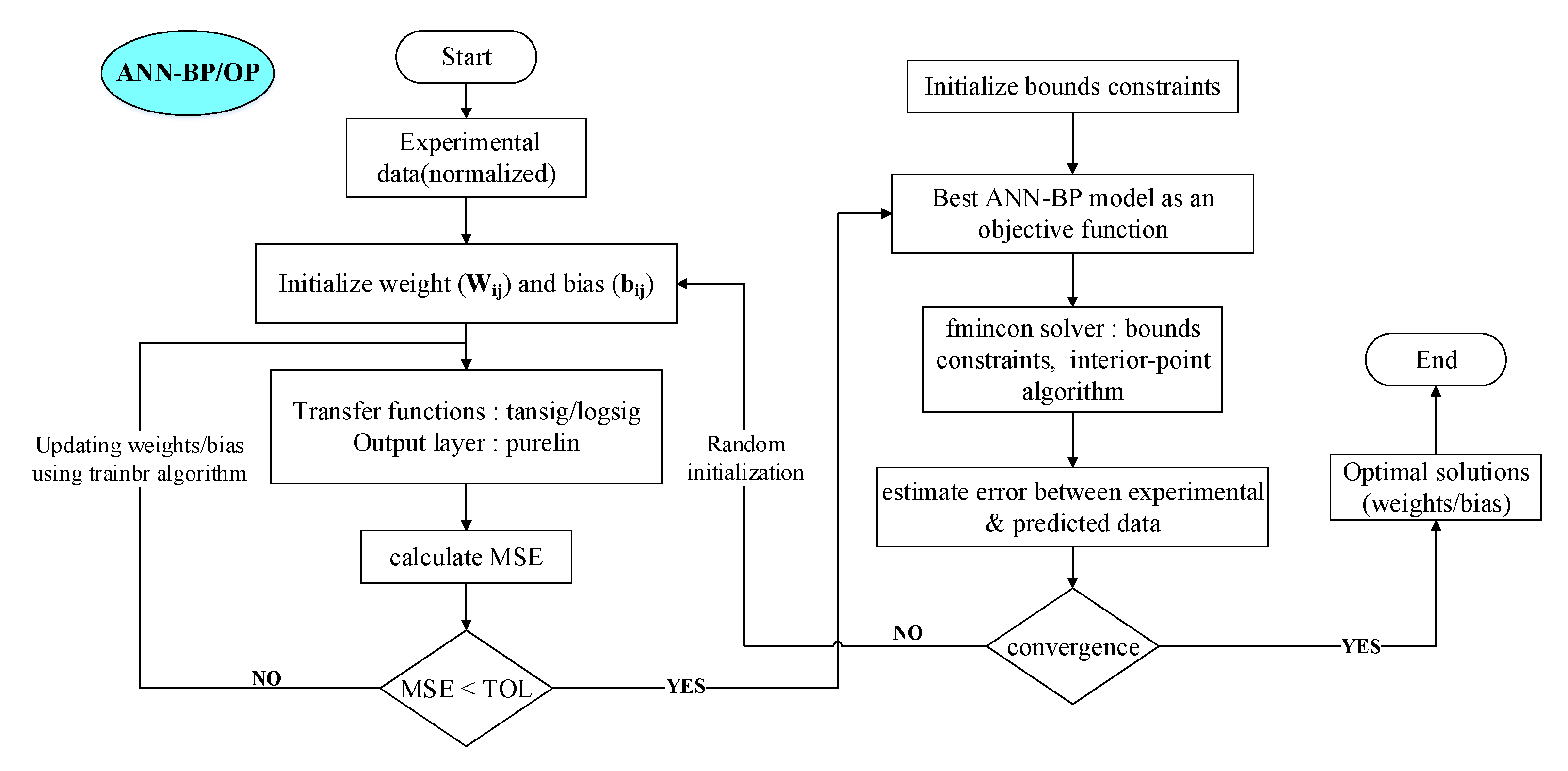
In the neural network model, the training process is carried out using an iterative process, which means in each step the model is updated with small weights and biases, for finding an optimum set of weights and biases to improve the model performance. A general approach for solving the neural network problem is to restart the training process multiple times with different random initial weights and biases, and allow the searching algorithm to find distinct candidates for the best trained ANN-BP model. This process is usually called multiple restarts. In this research work, the multiple restarts process was modeled by employing hybrid optimization procedures for training a network model in terms of adjusting weights and biases to predict the flow stress of medium carbon steel material under hot deformations as shown in
Figure 6. The nonlinear programming function, find minimum of constrained nonlinear multivariable function (fmincon), was utilized considering the interior-point (IP) algorithm to minimize AARE between an ANN-BP model and the desired flow stress data; the bounds constrained optimization procedures exploited in this work is also depicted in
Figure 7. The IP algorithm was selected due to its advantage in finding the minimum of a function within the presence of bounds constraints. Moreover, the benefits of exploiting this fmincon function rather than GA is that the computational time to solve the problem can be minimized without compromising the accuracy of results eventually. Wang et al. [
42] stated that in their research, the optimization problem based on fmincon function immensely reduced the calculation time related with GA, and also they pointed out that the obtained results was found to be reasonable against the actual results. In general, it is difficult to mention whether using wide range of bounds are valid or not at the first place. Therefore, at start of the optimization process, the problem was tested with a small range of bounds and then increased a little wider for allowing the process to be sampled extensively before selecting a valid candidate for a better solution. The limits of bounds constraints are selected from the trail experience for solving the optimization problem; the general form of optimization procedures are expressed below:
At start of the optimization process, the initial points are given randomly in order to begin optimization. At next step, the fmincon function automatically alters the
points strictly between the bounds constraints. Subsequently, the optimization algorithm searches through a bounds space of feasible values for the neural network model for a set of weights and biases that results in good performance on the model outcome. The optimization problem for activation functions is terminated when there is no improvement in the solution towards feasible directions and also the constraint tolerance is satisfied within the specified margin. The best candidate solutions for tansigmoid function in the hidden layer are obtained when the iterations and the function counts are 14 and 183, respectively, whereas for logsigmoid function, the numbers are computed as 5 and 71, respectively. The optimum solutions of AARE with transfer functions, tansig, and logsig, are achieved as 1.123% and 1.502%, respectively. The optimal results computed from the proposed ANN-BP/OP model are tabulated in
Table 5.
Table 4 and
Table 5 are strong evident that the prediction error obtained from the optimized network model varies from 0.728% to 1.775%, whereas for the basic network model, errors are ranging from 0.8637% to 2.172%, which states that the optimized ANN-BP model can correlate the material flow behavior more effectively than the conventional network model. In addition, there was no considerable differences between tansigmoid and logsigmoid functions with regard to the prediction error, but somehow, the optimum network model with tansigmoid function looks a little significant as far as reduction in the prediction error is concerned.
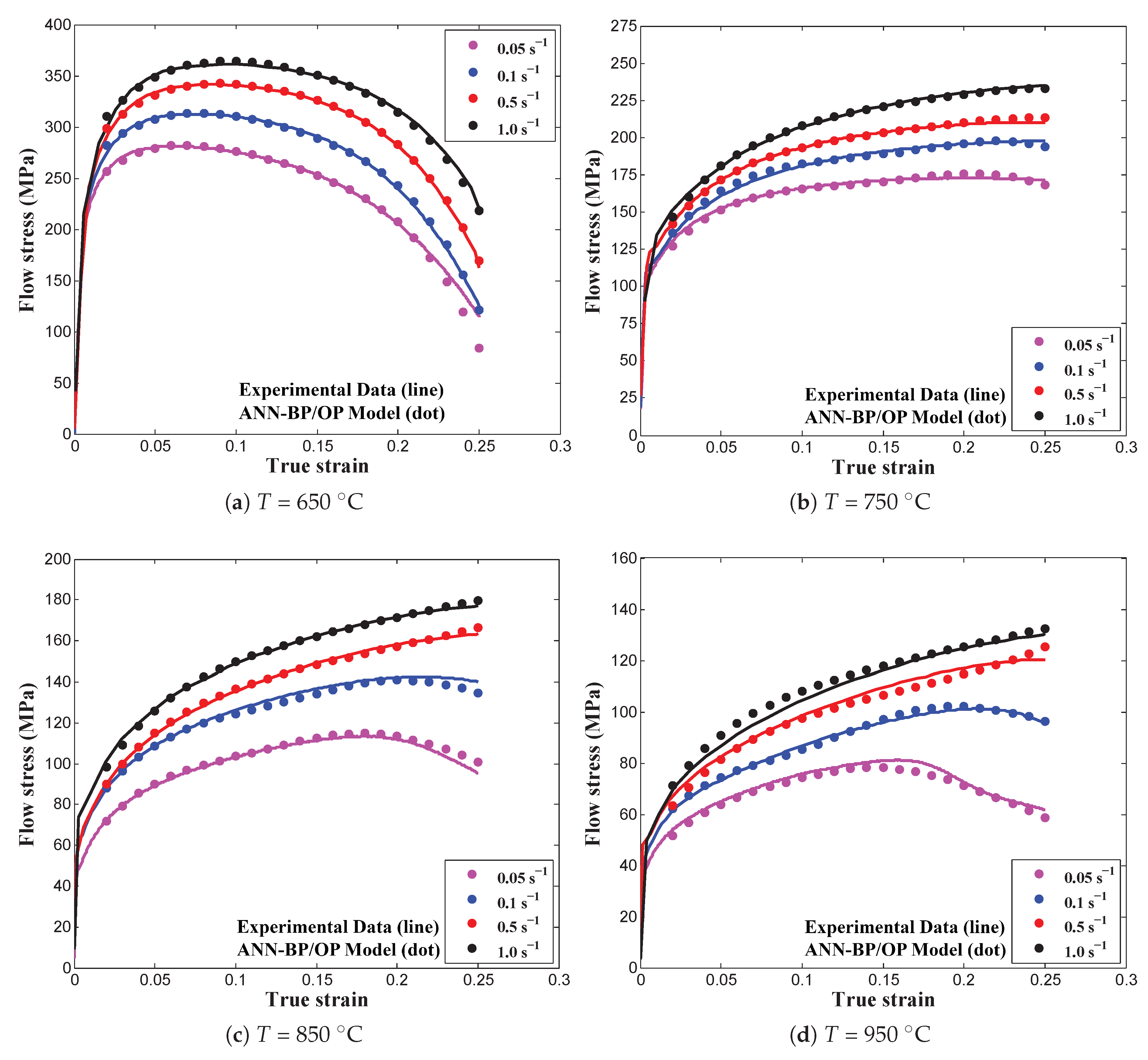
As can be seen in
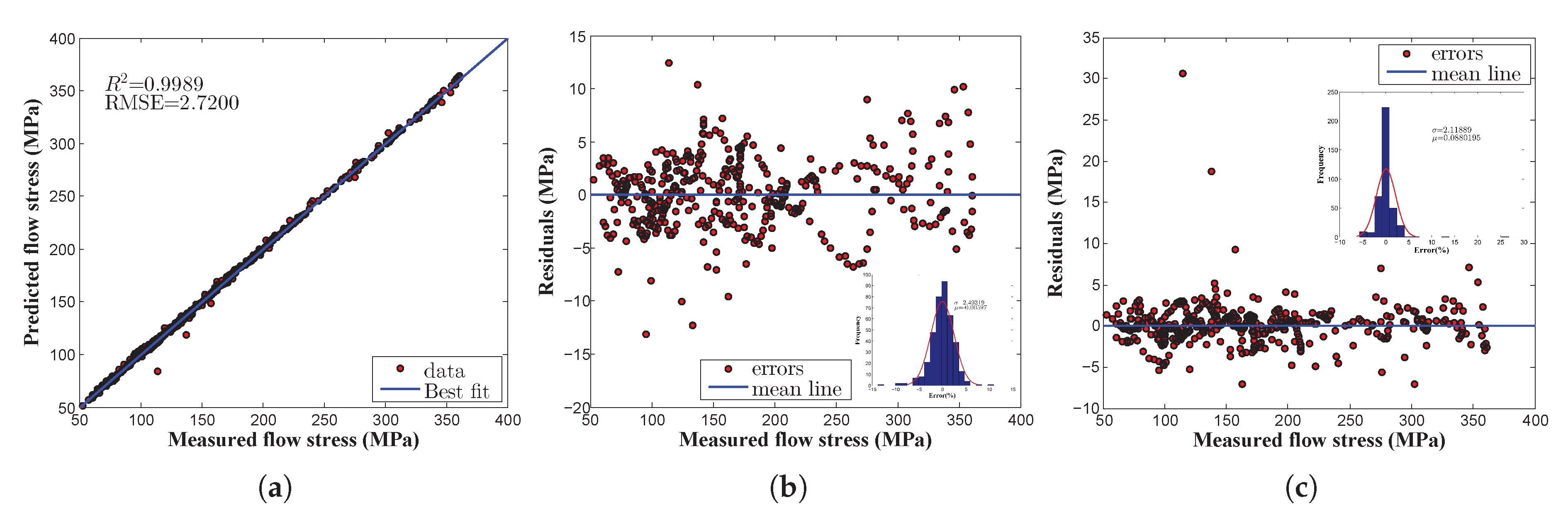
Figure 8, most of the predicted data points from the optimized ANN-BP model were close to the experimental measurements and this finding confirms the capability of the optimized flow stress model compared to the conventional network model. The correlation between experimental observations and the predicted is interesting because the computed data points almost followed the same trend line along the desired values as illustrated in
Figure 8. Moreover,
Figure 9a shows that the proposed model displayed a better correlation with respect to the measured data along with a better correlation coefficient
value at 0.9989. In addition, the statistical measurements,
and AARE, were estimated for each test condition using the proposed model as summarized in
Table 5 and likewise, it displays the excellent prediction ability of the proposed network model.
Figure 9b,c displays the random distribution of residuals with respect to zero error line; also, from the histogram plot (inset images), the distribution of residuals was noticed to be random and the probability distribution was found to be normal inside the working space. Furthermore,
Figure 9c conveys that even after the optimization process, the residual plot showed a fairly random pattern, which indicates that the proposed model provided a modest fit to the desired data. In addition, in order to clearly depict the model performance, the prediction error comparison using an ANN-BP and an ANN-BP/OP was modeled at different deformation temperatures and strain rates as shown in
Figure 10a.
According to our findings, the developed ANN models can be effectively applied to predict the material deformation behavior of medium carbon steel. Also the prediction error variations occurred in the traditional flow stress models [
8,
9], as shown in
Figure 10b, that introduced by the plastic instability phenomenon can be eliminated. Overall, the presented discussion implies that the proposed ANN-BP model has more impact to deal with a nonlinear experimental data than that of the conventional flow stress models in order to approximate the constitutive relationship of medium carbon steel at hot working conditions.


