Dynamic Uniform Deformation for Electromagnetic Uniaxial Tension

Abstract

To compare with quasi-static uniaxial tensioning, researchers designed an electromagnetic uniaxial tension method using a runway coil. However, the requirements to obtain a uniformly deformed sample and the ways the stress changes on the sample using a runway coil have not been studied in the past. In this study, a three-dimensional (3D) sequential coupling method was developed to analyze the factors affecting on-sheet deformation inhomogeneity under electromagnetic uniaxial tension. Two main process parameters, comprising the die type and the relative position of the coil and sheet, were evaluated. Under the optimal parameters, the experiment and simulation both obtained uniformly deformed samples with different discharge conditions, and the simulation method had a high accuracy in modeling the deformation process. The stress state of the sample is approximately unidirectional tensile stress before 240 μs. After 240 μs, the three main stresses showed significant oscillations.

1. Introduction

Both the automobile and aerospace industries use large-scale, advanced manufacturing methods that ideally minimize energy consumption and environmental impact in general. Low-density materials with good strength properties, such as aluminum alloys, help to achieve these goals. The main disadvantage of aluminum alloys is their poor formability relative to steel in conventional forming processes. Several studies have indicated that the formability of aluminum alloy increases dramatically when it is formed by high-speed processes.

Electromagnetic forming (EMF) is one of the most widely used high-speed forming methods, which can accelerate workpiece deformation by applying a magnetic force according to the electromagnetic induction theorem. A detailed review by Psyk et al. [1] showed that EMF has several advantages compared with conventional quasi-static forming, such as increased forming limits. Many scholars have proven that the formability of various materials can be dramatically increased under EMF, such as aluminum [2], steel [3], magnesium [4], copper [5], and titanium [6].

To obtain bidirectional tensile stress on a sheet, the flat spiral circular coils were used to make the sheet bulge. Imbert et al. [2] performed EMF experiments with AA5754 and AA6111 sheets, and found that strain states beyond the quasi-static forming limit diagram could be achieved using EMF. Li et al. [6] found that the forming limit of Ti-6Al-4V sheets increased by 24.37% when subjected to electromagnetic free bulging compared with quasi-static methods. Fang et al. [7] used electromagnetic pulse-assisted incremental drawing to obtain a large height-diameter ratio. Compared with the conventional drawing method, the height of the drawn cylinder was increased by 116% relative to the cylinder drawn by a conventional process.

To obtain uniaxial tensile stress on a sheet, different coil structures were developed. Li et al. [8] designed special specimens to obtain a state of uniaxial tension by EMF using a single-turn coil. Li et al. [9] experimentally investigated the formability of AA5052 sheets in a combined quasi-static-dynamic tensile process using a flat coil containing two square spiral coils. It was found that the formability of the aluminum alloy sheets after the combined quasi-static-dynamic tensile process dramatically increased compared with quasi-static-processed tensile tests. Xu et al. [10,11] designed a flat spiral coil, which can be named a “runway coil”, to make AZ31 sheets uniaxially tensioned by EMF. Based on the experimental results, the strain state of uniaxial tension can be obtained. However, a deformed sample with incomplete symmetry can also be obtained.

Therefore, determining the factors that affect uniform uniaxial tension in a sample by EMF using a runway coil is a key problem. Further, determining how the stress changes in a sample during EMF is another question that should be answered. In this study, a three-dimensional (3D) sequential coupling method was used to analyze the factors affecting a sample’s deformation uniformity and to obtain the optimum process parameters for electromagnetic uniaxial tension.

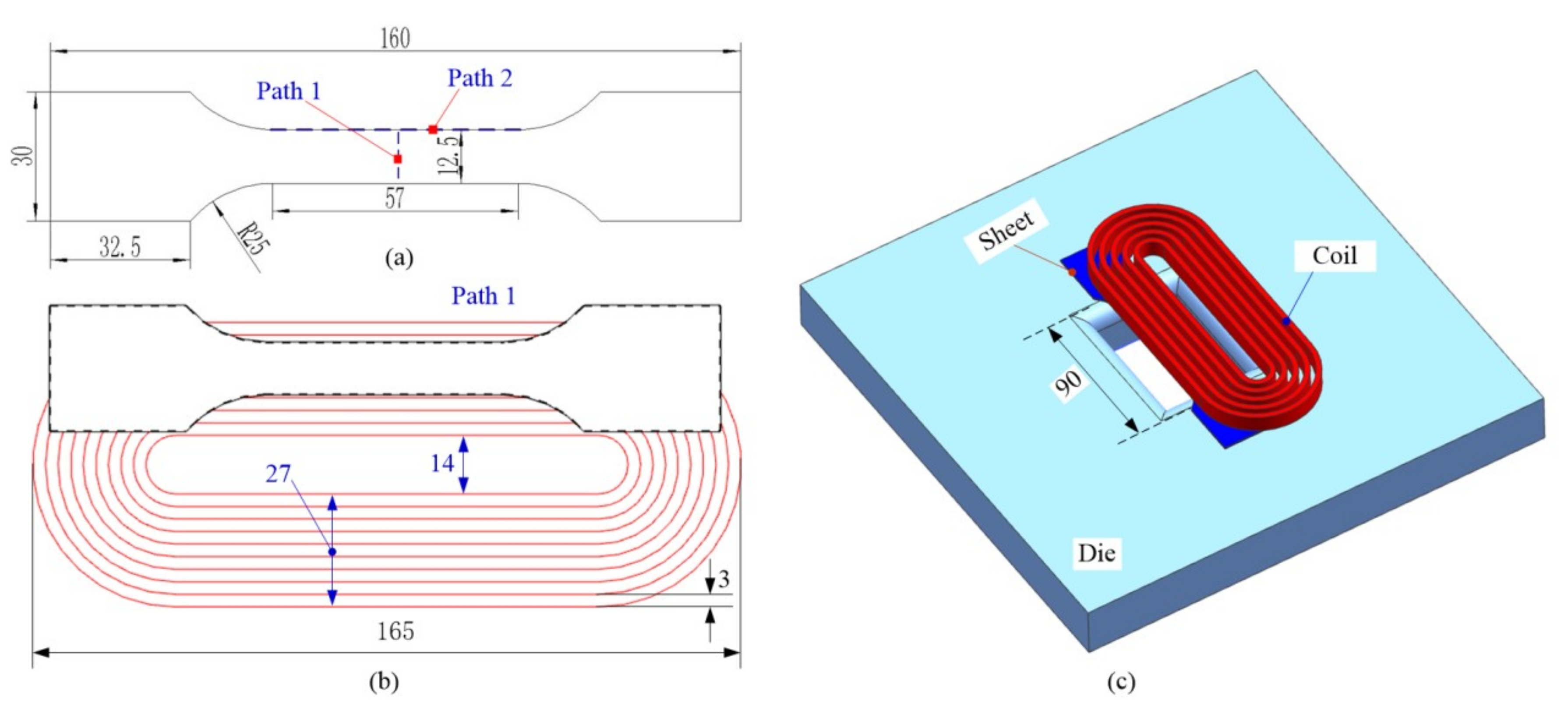
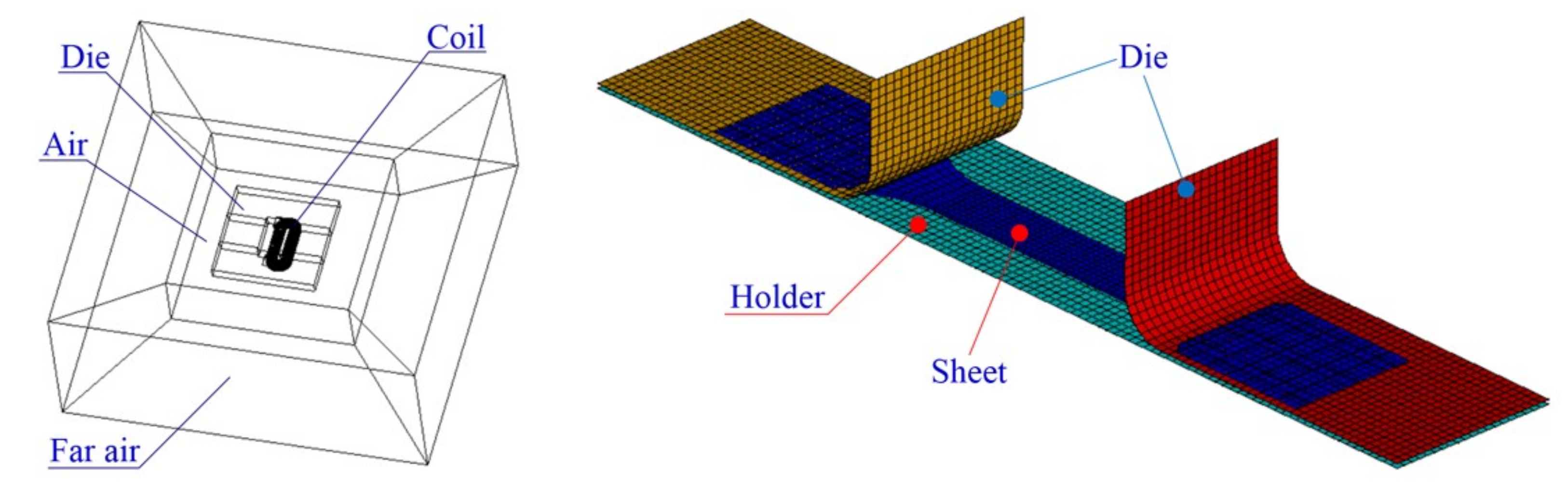
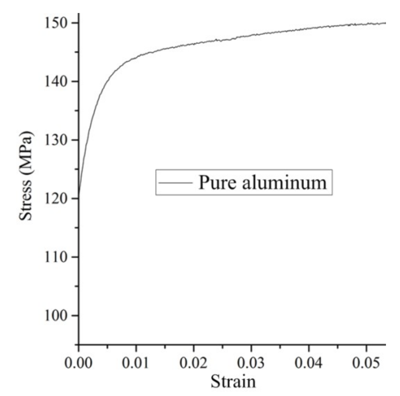
2. Experimental and Finite Element Simulation

The relative positions of the specimen, coil, and die are shown in Figure 1. A five-turn runway coil, combined with a capacitor bank, was used to obtain a unidirectional tensile stress state in the sheet material. The main parameters of the EMF equipment were the rated voltage (10 kV) and capacitance (1000 μF). The detailed experimental conditions were (1) the material (pure aluminum sheets with a high hardness; the elasticity modulus was taken as 0.68 GPa, Poisson’s ratio was taken as 0.33, and the density was taken as 2.7 × 10³ kg/m³) and (2) the gauged width and length of the tensioned specimens, which were 12.5 and 50 mm, respectively. The materials making up the coil core were a glass epoxy board with a rectangular-shaped groove and a copper wire with a section area of 3 × 10 mm², which was imbedded in the coil core. The length and width of the coils were 165 and 68 mm, respectively. The sheet was placed above a rectangular die. The length, width, and height of the die were 280, 280, and 30 mm, respectively. The die had an open rectangle window with dimensions of 70 × 50 mm² and an entry radius of 10 mm. To facilitate subsequent analysis, we defined path 1 and path 2 on the sample, as shown in Figure 1b.

Figure 2 shows the finite-element model established for magnetic-pulse uniaxial tension. ANSYS/EMAG software was used to calculate the magnetic force acting on the sheet. The electromagnetic field model consists of the far air region, air region, coils, die, and sheet. The sheet and coil were meshed into eight-node elements with the SOLID97 element type. The air region was meshed into tetrahedrons with the SOLID97 element type. In the mechanical model, ANSYS/LSDYNA software was used to simulate the dynamic deformation. During the forming process, the die and holder were treated as rigid bodies. Contact conditions were considered between the die and sheet, as well as between the sheet and holder.

For the EMF process, there are two main simulation methods for electromagnetic forming [12]: (1) the loose coupling method and (2) the sequential coupling method. If the magnetic forces are calculated based on the updated EM (electromagnetic) model, the simulation approach can be deemed to be the sequential coupling method. Thus, the sequential coupling method was adopted in this paper due to its higher accuracy. According to the electromagnetic induction theorem, the formula for the induced current and electromagnetic force on the sheet is as shown in Equations (1)–(3) [13]:

$$\frac{1}{\mathsf{\mu }}(\nabla \times B)=\nabla \times H=J$$

(1)

$$f=J\times B=\frac{1}{\mathsf{\mu }}(\nabla \times B)\times B$$

(2)

$$F=\frac{1}{\mathsf{\mu }}{\displaystyle \int (\nabla \times B)}\times B\cdot dV$$

(3)

where µ is the permeability (H/m), B is the magnetic flux (Wb/m²), H is the magnetic intensity (A/m), J is current density (A/m²), f is the magnetic force per unit volume (N/m³), V is the volume (m³), and F is the magnetic force (N).

Pure aluminum sheets with a high hardness were used in all the experiments. One millimeter thick standard specimens were used.

Table 1. Chemical composition of the main impurities of a pure aluminum sheet.

Element	Fe	Cu	Mg	Mn	Ga	Cr	K
wt. %	0.24	0.013	0.011	0.0055	0.019	0.0099	0.01

shows the chemical composition of the main impurities of a pure aluminum sheet. The engineering stress and strain can be obtained by tensile tests at room temperature. The true stress and strain can be calculated by Equations (4) and (5). Thus, the true stress-strain curve of pure aluminum under quasi-static conditions can be seen in Figure 3.

$${\mathsf{\sigma }}_{\mathrm{T}}={\mathsf{\sigma }}_{\mathrm{e}}(1+{\mathsf{\epsilon }}_{\mathrm{e}})$$

(4)

$${\mathsf{\epsilon }}_{\mathrm{T}}=\ln (1+{\mathsf{\epsilon }}_{\mathrm{e}})$$

(5)

where σ_T is the true stress, σ_e is the engineering stress, ε_T is the true strain, and ε_e is the engineering strain.

To consider the effect of a high strain rate on forming, the behavior of a viscoplastic material was modeled with a rate-dependence law (the Cowper-Symonds constitutive model) in the ANSYS/LSDYNA finite-element analysis software. Thus, the Cowper-Symonds constitutive model was used to model the high-speed forming, as shown in Equation (6):

$$\mathsf{\sigma }={\mathsf{\sigma }}_{\mathrm{s}}(1+{(\frac{\dot{\mathsf{\epsilon }}}{P})}^m)$$

(6)

where σ is the dynamic flow stress, σ_s is the quasi-static constitutive behavior of the sheet (cf. Figure 3), $\dot{\mathsf{\epsilon }}$ is the strain rate, P = 6500 s⁻¹, and m = 0.25 is the specific parameter of the aluminum alloy.

3. Results

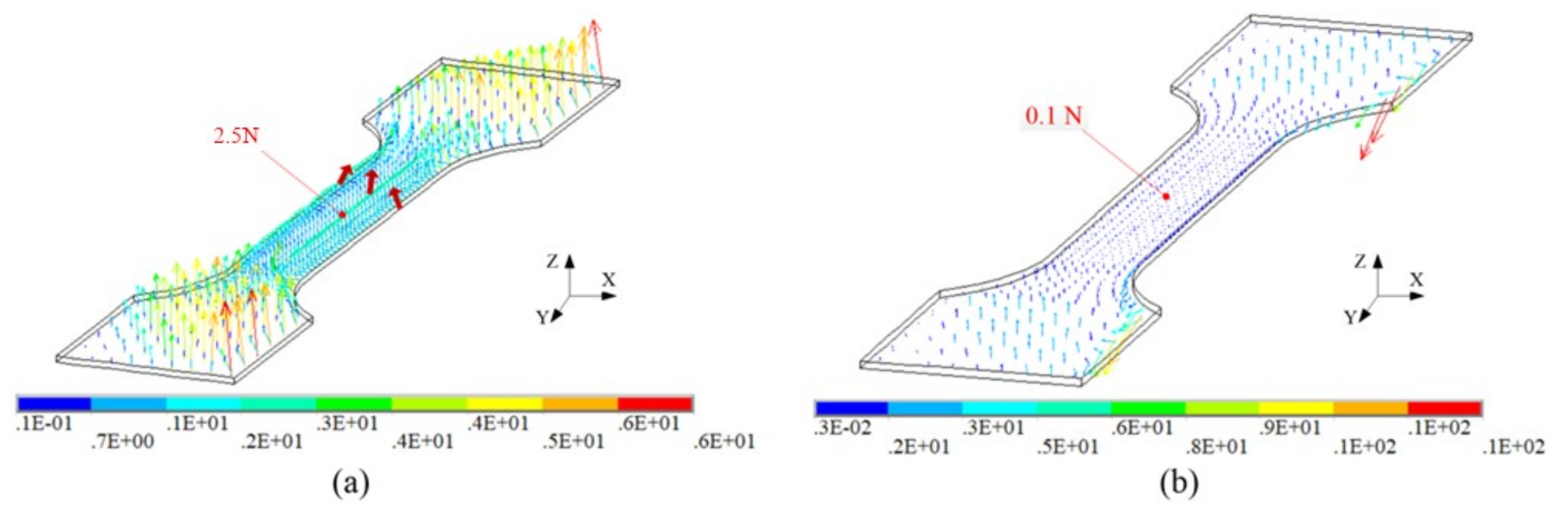
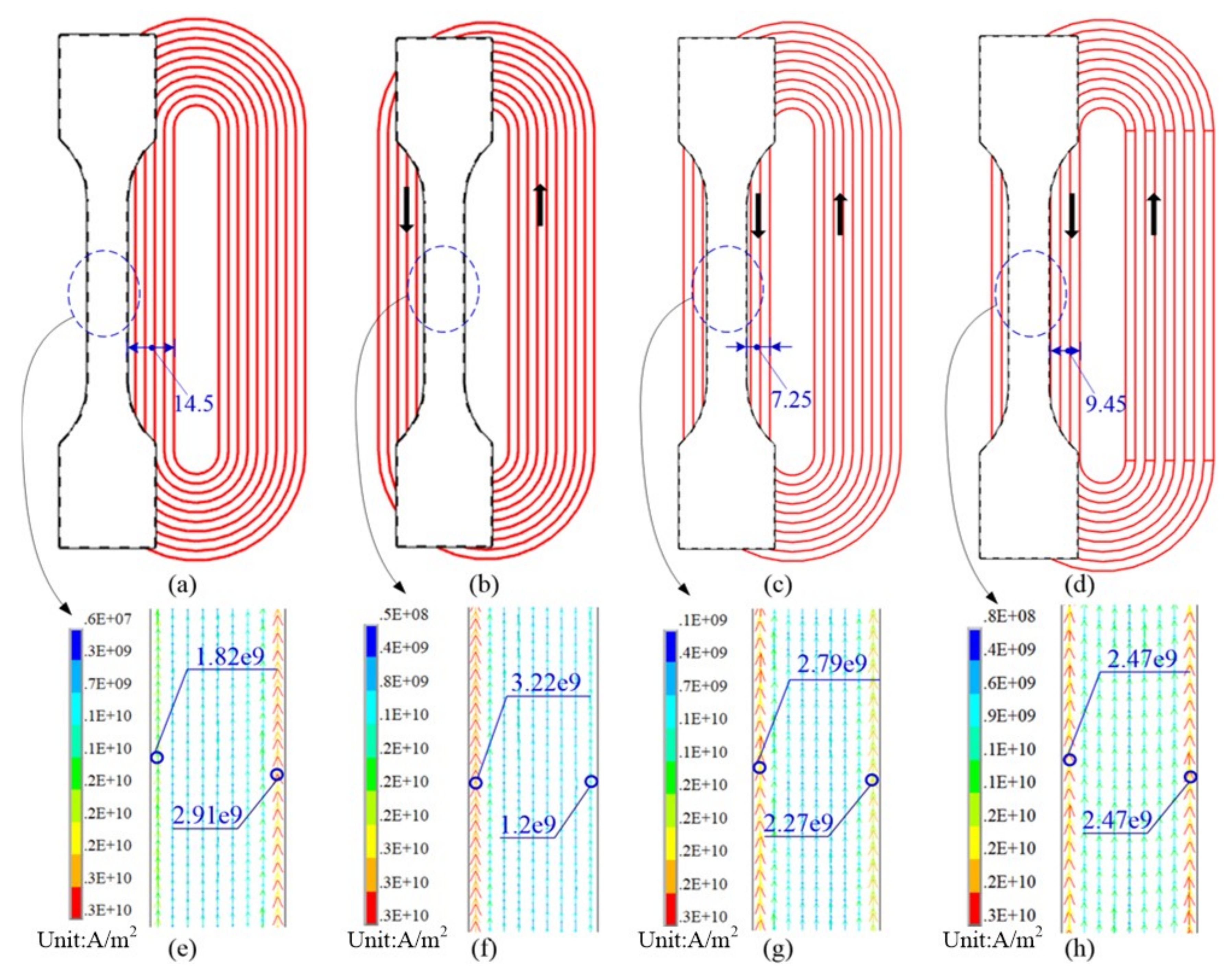
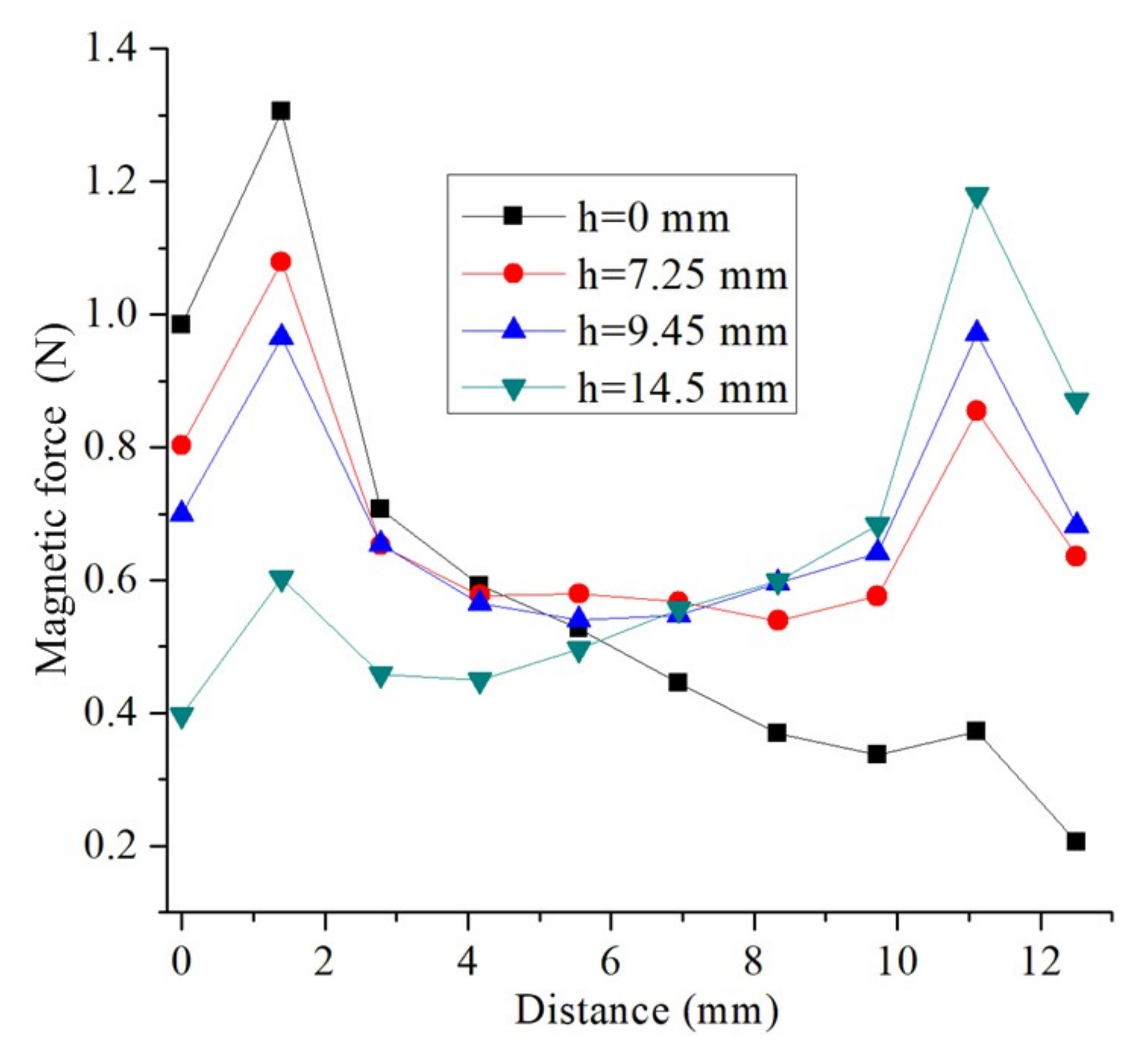
3.1. Effect of Die on Current Distribution and Magnetic Force

To prove that the effect of the die shown in Figure 1 can significantly affect the current distribution on the sample, two sets of dies were selected: (1) a conductive die made of Q235 steel and (2) a nonconductive die made of epoxy plate. Figure 4a shows the current curves through the coil, measured using a Rogowski coil. A higher current amplitude and the same pulse width were obtained at a higher discharge voltage by using a nonconductive die made of epoxy plate. Compared with the nonconductive die made of epoxy plate, the current amplitude and pulse width obtained by using the steel die were larger and smaller at 1250 V, respectively. This is because coil discharging not only produces electromagnetic induction to the sheet, but also to the steel die. As the induction current on the steel die is opposite to the current passing through the coil, the steel die will generate mutual inductance with the coil, reducing the inductance of the entire system. Thus, the current amplitude obtained using the steel die was higher than that obtained using the epoxy die. Figure 4b shows a schematic diagram of counterclockwise current loaded on the coil. To facilitate subsequent analysis, we defined the distance between the right-end face of sample and the coil’s inner turn as h, as shown in Figure 4b.

Figure 5 shows the current density and current direction distributions on the sheet and die at 20 μs. In the case of the steel die, the sample and die constituted a clockwise current loop, the current in the middle of the sample was almost equal, and the current in the two side ends is slightly larger in the sample. In the case of the epoxy die, the induced current on the sample itself constituted a clockwise current loop within the sample because the epoxy die is not conductive. The current near the edge of the side arc was larger than that in the central area of the sheet, and the current directions on each side end of the sheet were opposite.

Figure 6 shows the magnitude and direction of the magnetic force on the sheet at 20 μs. In the case of the steel die, the magnetic force acting on the sample was generally in the positive direction of the Z-axis, and the magnetic force on the central region of the sample was evenly distributed. In the case of the epoxy die, the magnetic force acting on the middle of the sample was too small. This is because the magnetic force is related to the current distribution on the sheet. According to the simulation results shown in Figure 5; Figure 6, a steel conductive die made of Q235 steel was used in the following simulation and experiment.

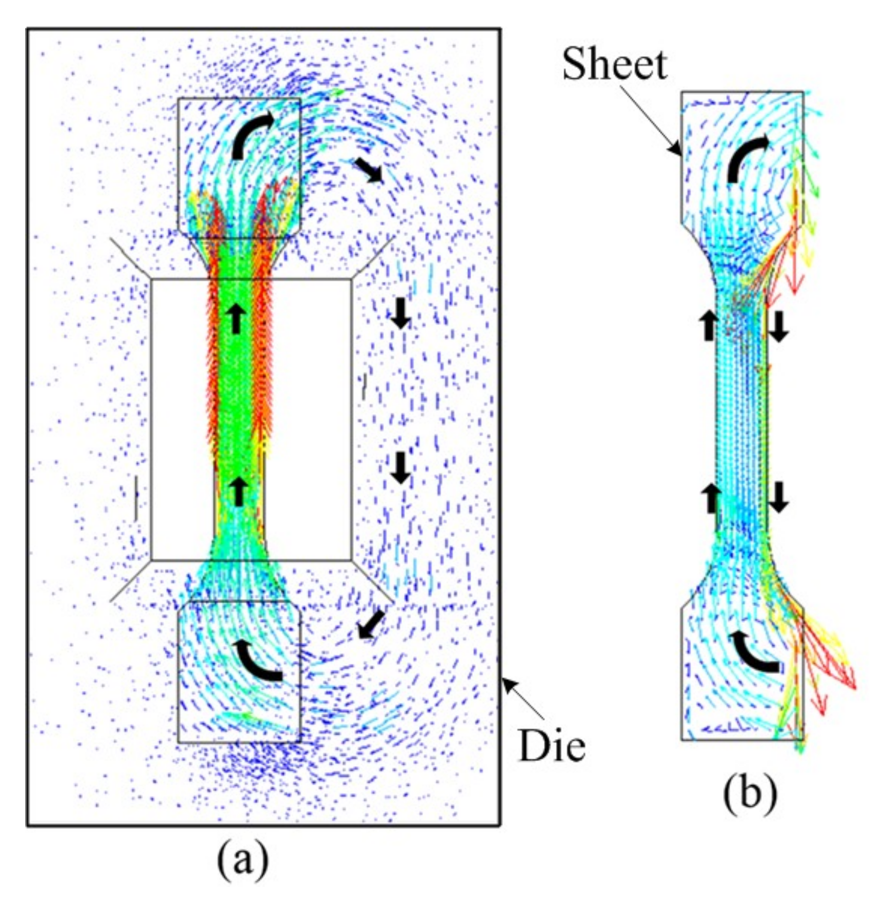
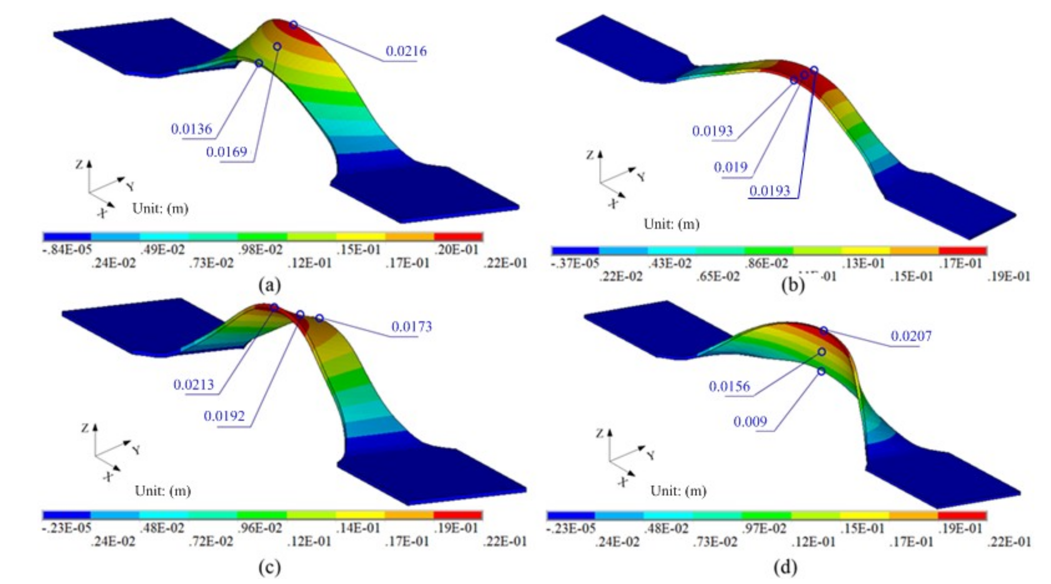
3.2. Effect of the Relative Position of the Coil and Sample on the Deformation

Figure 7 shows the relative position of the sample to the coil. The width of the left half of the coil is 27 mm, and the width of the sample is 12.5 mm. If h = 14.5 mm, the left side of the straight edge of the sample overlaps with the leftmost side of the coil, as shown in Figure 7a. Figure 7e shows the current flow direction and current in the middle of the sample. The current density on the left side of sample was far less than that on the right side of sample. This is because there were more wires on the right side of the sample. If h = 0 mm, the right side of the straight edge of the sample coincides with the right side of the left part of the coil, as shown in Figure 7b. Figure 7f shows the current flow direction and intensity in the middle of the sample shown in Figure 7b. The current density on the left side of the sample was much higher than that on the right side of the sample. If h = 7.25 mm, the middle axis of the sample overlaps with the middle axis of the left half of the coil. Figure 7g shows the current flow direction and intensity in the middle of the sample, using the condition shown in Figure 7c. The current density on the left side of the sample was higher than that on the right side of the sample. This is because the right side of the coil was close to the left side of the coil, and the current flowing through the right side of the coil was opposite to the current flowing through the left side of the coil; therefore, the current density on the left side of the sample was higher than that on the right side of the sample. When h = 9.45 mm, the current densities on both sides of the straight edge of the sample were the same and higher than the current density in the middle of the sample. Therefore, the entire current density was symmetrically distributed on the sheet, as shown in Figure 7d,h.

Figure 8 shows the relative position of the sample and coil and the effect of the magnetic force on path 1. The distribution of magnetic force was similar to the current density shown in Figure 7. Therefore, the higher the current density, the higher the magnetic force acting on the sample. Only when h = 9.45 mm, the magnetic force on Path 1 became symmetrically distributed.

Figure 9 shows the effect of the relative positions of the sheet and coil on the final sheet shape. When h = 0, 7.25, and 14.5 mm, because of the asymmetric distribution of magnetic force on the sheet, the sheet shape was distorted. In particular, when h = 0 mm, the magnetic force acting on the left side of the sheet was significantly higher than that on the right side of the sheet, and the deformation on the left side of the strip was significantly higher than that on the right side of the strip. When h = 14.5 mm, the deformation on the right side was significantly higher than that on the left side. When h = 9.45 mm, the displacements of the left, middle, and right ends of the highest point of the sheet were 19.3, 19, and 19.3 mm, respectively. The central deformation of the sheet was ~1.5% smaller than that of the left and right ends of sheet.

Figure 10 shows the effect of the relative position of the sheet and coil on path 1. When h = 0, 7.25, and 14.5 mm, the deformation on Path 1 was linear. When h = 9.45 mm, the sheet was symmetrically distended on both sides, and the deformation was symmetrical.

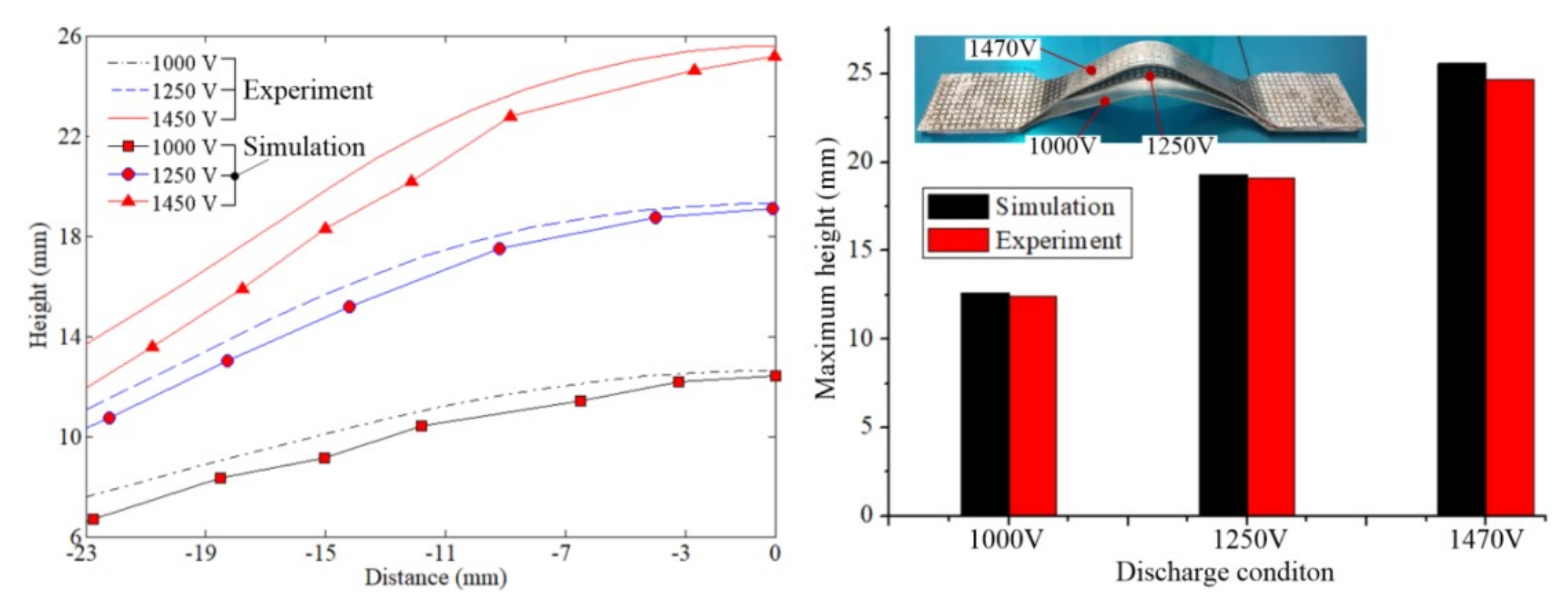
3.3. Comparison of Experimental and Simulation Results

Based on the above simulation results, the steel conductive die made of Q235 steel and the relative distance h = 9.45 mm were chosen. Figure 11 shows the profiles of path 2 and the maximum heights obtained from the experiment and simulation at different discharge voltages. The profiles between the experiment and simulation showed only a slight deviation and a small error at the sheet peak under different discharge voltages. Therefore, the simulation method had a high accuracy to predict the dynamic deformation from electromagnetic uniaxial tension.

4. Discussion

At a discharge voltage of 1250 V, Figure 12a shows the equivalent plastic strain distribution on the sample when the deformation was terminated. The maximum equivalent plastic strain was 0.193. To facilitate subsequent analysis, the special nodes and elements shown in Figure 12a were extracted. Figure 12b–d shows the changes in the equivalent plastic strain, deformation height, and velocity with time at the special nodes. At time t = 240 μs, the equivalent plastic strain at special nodes reached a maximum and no longer changed. It can be considered that t = 240 μs represents the end of deformation. However, after t = 240 μs, the velocity and displacement of nodes on the sample still varied slightly.

Figure 13 shows the changes in the three principal stresses at special nodes with time. Some phenomena can be found at 0–240 μs: (1) the first principal stress at the three special nodes gradually increased, and the direction of the first principal stress is the tangential direction on the sample; (2) the second principal stress at the three special nodes was very small, and the direction of second principal stress was the width direction on the sample; (3) the third principal stress at the three special nodes was less than zero due to the magnetic pressure acting on these nodes. The magnitude of the third principal stress was much less than the first principal stress and the direction of the third principal stress was normal to the sample. Due to the second and third principal stresses both being much smaller than the first principal stress, the deformation process can be approximately considered as a uniaxial tensile stress state. After 240 μs, the three main stresses at the special nodes showed significant oscillations.

When the sheet was bent, the maximum stress of the sheet was usually at a tangent to the sheet. However, when the high-frequency shock occurred, the stress on the plate was disordered. To analyze the magnitude and direction of the principal stress on the sheet at different times more clearly, six elements in Figure 12a were extracted for the following analysis. Figure 14 shows the changes in stresses with time at six special elements. At a time of 180 μs, all the six elements were subjected to tangential tensile stress above 240 MPa, and the stresses in the width and thickness directions were very small. Therefore, the sheet deformation can be considered as a unidirectional tensile state. At 260 μs, the sheet top element (ELEM 468, 460) was still subjected to tangential tensile stress; however, the tangential tensile stress decreased to 33.5 MPa and 30 MPa. However, the elements (ELEM 612, 604, 756, and 748) were subjected to a higher tangential compressive stress. At 320 μs, the sheet top elements (ELEM 468 and 460) were subjected to the tangential tensile stress; however, the tangential tensile stress increased to 205 MPa and 219 MPa, respectively. At 360 μs, the stress direction of top element (ELEM 468 and 460) changed from tensile stress to compressive stress; however, the tangential compressive stresses were 84 and 27 MPa, respectively. At 360–500 μs, the stress on the top elements (ELEM 468 and 460) was still a lengthwise compressive stress; however, the value of the compressive stress continuously changed. Comparing the other elements (ELEM 612, 604, 756, and 748), the stress direction on each unit still alternately changed from tensile to compressive stress, and the magnitude also changed constantly. The dynamic changes in the stress generally significantly decreased the lengthwise stress on the sheet compared with that at 180 μs. At 2000 μs, the residual lengthwise stress on the sheet was not only small, but also both lengthwise tensile and compressive stresses existed on the outer surface of the sheet.

5. Conclusions

In this study, a 3D sequential coupling method was developed to analyze the factors affecting on-sheet deformation inhomogeneity using runway coils. Compared with the experimental results under different voltages, the simulation results had high accuracy and precision. Some conclusions can be obtained as follows:

(1)

The die has a significant effect on the current distribution in the sample. Compared with a nonconductive die, the same current direction with similar current intensity in the sample can be obtained with a steel die.

(2)

The symmetrical distribution of magnetic force on path 1 can be obtained by adjusting the relative position of the sample and coil. Subsequently, the sheet deforms with a uniform 3D shape.

(3)

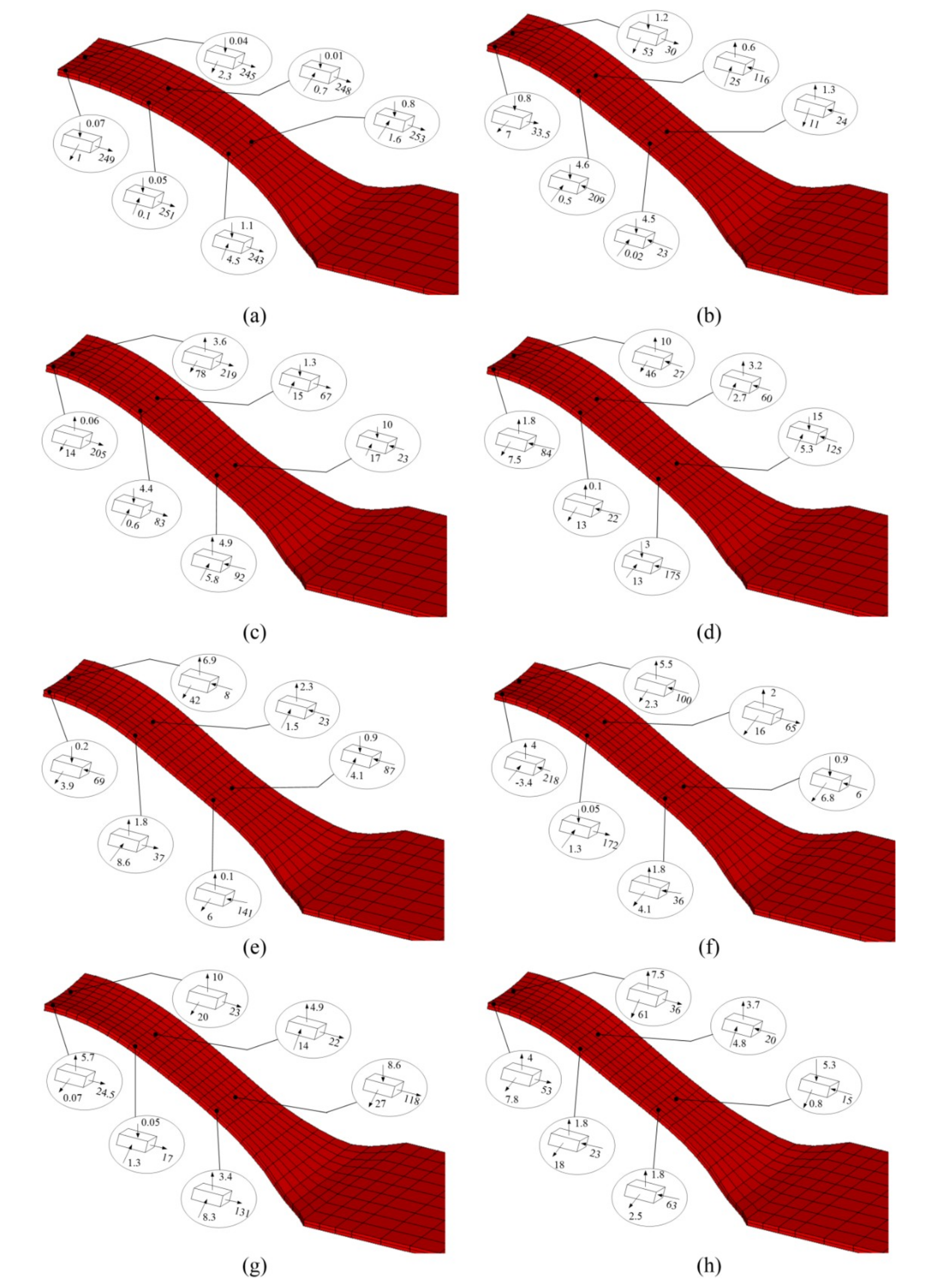
The deformation process can be approximately considered as a uniaxial tensile stress state before 240 μs. After 240 μs, the three main stresses at the special nodes showed significant oscillations.

References

1. Psyk, V.; Risch, D.; Kinsey, B.L; Tekkaya, A.E.; Kleiner, M. Electromagnetic forming—A review. J. Mater. Process. Technol. 2011, 211, 787–829. [Google Scholar] [CrossRef]
2. Imbert, J.M.; Winkler, S.L.; Worswick, M.J.; Oliveira, D.A.; Golovashchenko, S. The effect of tool-sheet interaction on damage evolution in electromagnetic forming of aluminum alloy sheet. J. Eng. Mater. Technol. 2005, 127, 145–153. [Google Scholar] [CrossRef]
3. Seth, M.; Vohnout, V.J.; Daehn, G.S. Formability of steel sheet in high velocity impact. J. Mater. Process. Technol. 2005, 168, 390–400. [Google Scholar] [CrossRef]
4. Meng, Z.H.; Huang, S.Y.; Hu, J.H.; Huang, W.; Xia, Z.L. Effects of process parameters on warm and electromagnetic hybrid forming of magnesium alloy sheets. J. Mater. Process. Technol. 2011, 211, 863–867. [Google Scholar] [CrossRef]
5. Jiang, H.W.; Ni, L.; Xiong, Y.Y.; Li, Z.G.; Liu, L. Deformation behavior and microstructure evolution of pure Cu subjected to electromagnetic bulging. Mater. Sci. Eng. A 2014, 593, 127–135. [Google Scholar] [CrossRef]
6. Li, F.Q.; Mo, J.H.; Li, J.J.; Zhou, H.Y. Formability of Ti-6Al-4V titanium alloy sheet in magnetic pulse bulging. Mater. Des. 2013, 52, 337–344. [Google Scholar] [CrossRef]
7. Fang, J.X.; Mo, J.H.; Cui, X.H.; Li, J.J.; Zhou, B. Electromagnetic pulse-assisted incremental drawing of aluminum cylindrical cup. J. Mater. Process. Technol. 2016, 238, 395–408. [Google Scholar] [CrossRef]
8. Li, G.Y.; Deng, H.K.; Mao, Y.F.; Zhang, X.; Cui, J.J. Study on AA5182 aluminum sheet formability using combined quasi-staticdynamic tensile processes. J. Mater. Process. Technol. 2018, 255, 373–386. [Google Scholar] [CrossRef]
9. Li, C.; Liu, D.; Yu, H.; Ji, Z. Research on formability of 5052 aluminum alloy sheet in a quasi-static–dynamic tensile process. Int. J. Mach. Tools Manuf. 2009, 49, 117–124. [Google Scholar] [CrossRef]
10. Xu, J.R.; Yu, H.P.; Li, C.F. An Experiment on Magnetic Pulse Uniaxial Tension of AZ31 Magnesium Alloy Sheet at Room Temperature. J. Mater. Eng. Perform. 2013, 22, 1179–1185. [Google Scholar] [CrossRef]
11. Xu, J.R.; Lin, Q.Q.; Cui, J.J.; Li, C.F. Formability of magnetic pulse uniaxial tension of AZ31magnesium alloy sheet. Int. J. Adv. Manuf. Technol. 2014, 72, 665–676. [Google Scholar] [CrossRef]
12. Cui, X.H.; Mo, J.H.; Li, J.J.; Huang, L.; Zhu, Y.; Li, Z.W.; Zhong, K. Effect of second current pulse and different algorithms on simulation accuracy for electromagnetic sheet forming. Int. J. Adv. Manuf. Technol. 2013, 69, 1137–1146. [Google Scholar] [CrossRef]
13. Cui, X.H.; Mo, J.H.; Han, F. 3D Multi-physics field simulation of electromagnetic tube forming. Int. J. Adv. Manuf. Technol. 2012, 59, 521–529. [Google Scholar] [CrossRef]
Figure 1. Schematic diagram of magnetic-pulse bending: (a) sample structure, (b) relative position of coil and sample, and (c) 3D structure of the forming process. Units: mm.
Metals 09 00425 g001
Figure 2. Finite-element models for magnetic pulse forming: (a) electromagnetic field model and (b) structure model.
Metals 09 00425 g002
Figure 3. Stress-strain curve.
Metals 09 00425 g003
Figure 4. Current through the coil: (a) current curves measured by Rogowski coil and (b) counterclockwise current loaded on the coil.
Metals 09 00425 g004
Figure 5. Current distribution after coil discharge at 20 µs: (a) using the conductive die and (b) using the nonconductive die.
Metals 09 00425 g005
Figure 6. Magnetic force distribution on the sample at 20 µs: (a) using the conductive die and (b) using the nonconductive die.
Metals 09 00425 g006
Figure 7. Effect of the relative position of the coil and sample on the current density with (a) h = 14.5 mm, (b) h = 0 mm, (c) h = 7.25 mm, and (d) h = 9.45 mm (e) current value with h = 14.5 mm (f) current value with h = 0 mm, (g) current value with h = 7.25 mm, (h) current value with h = 9.45 mm.
Metals 09 00425 g007
Figure 8. The relative position of the sample affected by the magnetic force on path 1.
Metals 09 00425 g008
Figure 9. Effect of relative position on final shape: (a) h = 14.5 mm, (b) h = 9.45 mm, (c) h = 7.25 mm, (d) h = 0 mm.
Metals 09 00425 g009
Figure 10. Deformation profiles on Path 1.
Metals 09 00425 g010
Figure 11. Experimental and simulation results: (a) the final profiles on path 2 and (b) the maximum height of the sample peak.
Metals 09 00425 g011
Figure 12. Dynamic deformation: (a) 3D shape and equivalent plastic strain, (b) plastic strain with time, (c) height with time, and (d) velocity with time.
Metals 09 00425 g012
Figure 13. Relationship between time and principal stress at special nodes: (a) node 305, (b) node 313, and (c) node 321.
Metals 09 00425 g013
Figure 14. Stress and direction at different times: (a) 180 μs, (b) 260 μs, (c) 320 μs, (d) 360 μs, (e) 420 μs, (f) 500 μs, (g) 1000 μs, and (h) 2000 μs.
Metals 09 00425 g014