Observation and Interpretation of Closely Spaced Fundamental Modes of a High-Rise Building

Abstract

In this paper the dynamic behaviour of a high-rise building with complex structural system is studied. In some cases, to optimize the building design, the horizontal stability of the building is accomplished by the contribution of several structural components. This is the case of the JuBi tower, the building studied in this paper. The horizontal stability of the building is accomplished by three cores and outer walls. The cores and the walls are connected through the floors and the foundation. The data recorded during the experimental campaign carried out in this building show a double-peak behaviour corresponding to two closely spaced modes in the translational directions. This is caused by the weak coupling between the structural components. To study this phenomena, in this paper, a yet unique double-beam model is used. The parameters of the model are tuned so as to resemble the experimental response of the building. Results of the model evidence that the weak coupling is caused by the beams and the foundation. Also, it is shown that the two closely spaced modes correspond both to bending shape modes.

1. Introduction

High-rise buildings can be subjected to vibrations caused by wind gusts. These vibrations may produce structural damage or lead to a drastic reduction of their fatigue life [1]. Therefore, it is an important aim for engineers and researchers to understand the dynamic behviour of structures. In this paper, the dynamic behaviour of a high-rise building is studied. The horizontal stability of the building is achieved by means of three cores of different dimensions and outer walls that are coupled through the floors and the foundation of the building. The floors are embedded to the walls and simply supported to the columns. The outer walls and cores are founded in a common foundation.

To study the dynamic behaviour of the building, first an extensive experimental campaign was carried out in the building. The experimental data shows a double-peak behaviour corresponding to two closely spaced resonance frequencies in the translational directions. The double-peak behaviour is caused by the fact that the configuration of the structural system creates a weakly coupled system. It is therefore of a great interest to understand the behviour of the weak coupling in the building. To this end, in this paper, a double-beam system is used as to resemble the dynamic response of the building under study.

Generally, double-beam systems consist of two one-dimensional beams connected by uniformly distributed discrete elements. Free vibrations of double-beam systems were studied by Seeling and Hoppmann [2], which provided solutions for natural frequencies and mode shapes. Forced vibrations solutions were also provided by Seeling and Hoppmann [3] under impact loading. Dublin and Friedrich [4] found the solution of forced vibrations of two continuous beams connected by distributed visco-elastic elements. Rao [5] studied the free response of two elastically connected Timoshenko beams considering the rotatory inertia. Vibrations in double-beam systems of non-identical beams with uniform boundary conditions were studied by Chonan [6], and Hamada [7] making use of the Laplace transform, and by Douglas and Yang [8] using the mechanical impedance format. Irie [9] solved the steady-state response of a double-beam system with internal damping under sinusoidal loading. Vu [10] presented solutions for double-beam system with arbitrary boundary conditions and general loading. Later, Oniszczuk [11] presented analytical solutions for free and forced vibrations of an undamped double-beam system with simply supported boundary conditions. More recently, Li and Sun [12], presented a solution for free and forced response, for different loading conditions, of non-identical beams elastically connected with arbitrary boundary conditions. All these systems are widely used to study vibrations in many applications, however, until now, no attempt has been made to use double-beam system to model a high-rise building.

Therefore, this paper presents a unique yet double-beam model to study structural vibrations of a high-rise building subject to wind loading. In the model, the beams, represent the cores and the outer walls. The beams are modelled with non-identical mass, bending stiffness and internal damping. These are connected with uniformly distributed visco-elastic elements that mimic the floors. At the bottom end, springs are used to represent the soil resistance in the translational and rotational directions. The capacity of dissipating energy in the soil is taken into account by means of a translational and rotational dashpots. To model the wind loading a spectrum for along-wind is used.

Having tuned the parameters of the model to the case study, this shows a good agreement compared to the experimental response. The results evidence that the weak coupling takes place mainly between the beams and the foundation of the building. The model also shows that the closely spaced modes correspond to bending modes.

2. Full-Scale Measurements

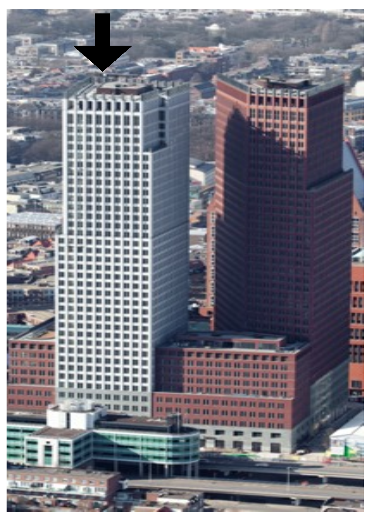
2.1. Building Description

The JuBi tower (see Figure 1) is a 146 m office building with 39 storeys located in The Netherlands. The building is designed with a tube-in-tube configuration, that provides the horizontal stability. The outer tube represents the outer walls and has an irregular shape that defines the area of the building. The inner tube is composed of three cores. The three cores have a rectangular shape, and are asymmetrically distributed within the outer tube area. The cores and the outer walls are connected by the simply supported concrete floors. These floors are weakly connected to the cores and outer walls, creating a weakly coupled system.

Ambient loads such as wind gusts, act on the outer walls, and this force is transferred to the cores through the floors and then directly to the foundation. Even though the building is surrounded by other buildings, the foundation is not connected to adjacent buildings.

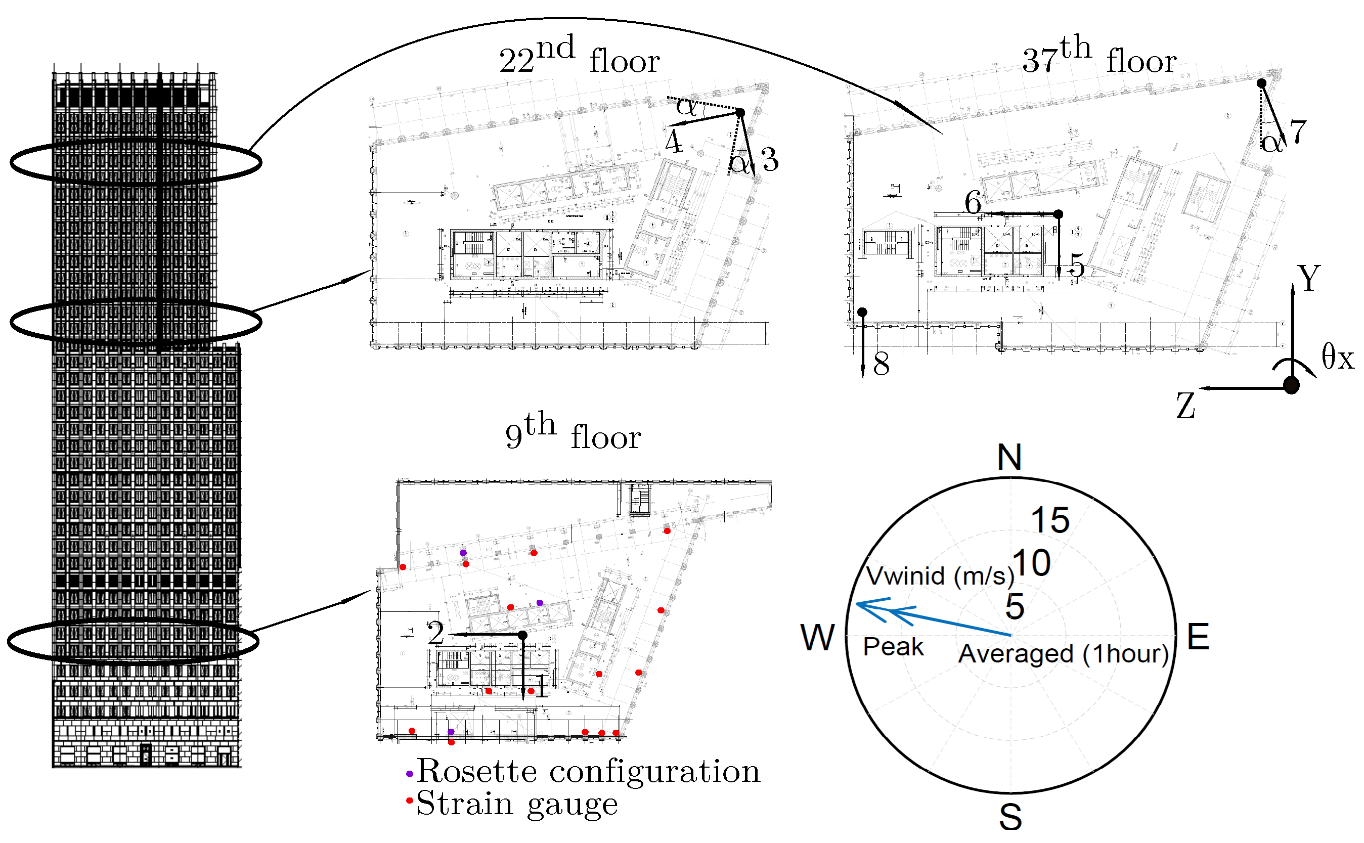
2.2. Instrumentation Strategy and Experimental Results

During an extensive measurement campaign acceleration and strain data were collected under strong wind conditions. To perform the measurements accelerometers at the 9th, 22nd and 37th floors, and strain gauges at the 9th floor were installed. The instrumentation strategy is shown in Figure 2. However, for the purpose of this work solely measurements at the top height (37th story) for a period of two hours will be used.

The 37th floor is instrumented with four accelerometers measuring in the weak, strong and torsional directions of the building. After some data processing time traces of each accelerometer can be obtained. Figure 3 shows the data registered by each sensor during 2 h of measurements.

The data plotted in Figure 3 shows that largest acceleration values are registered by sensor 5 during some events, which reveals that this can be the weak direction of the building. However, for some time periods it is difficult to distinguish if sensor 5 or sensor 6 registered larger accelerations. By plotting the data recorded by each sensor as shown in Figure 4, it can be observed that none of the two sensors is perfectly aligned with the weak vibrational direction of the building.

Given that, the power spectral density (PSD) of the velocity obtained by numerically integrating the acceleration measurements registered by the sensors 5 to 8 shown in Figure 3 shows that each sensor captures vibrations at all resonance frequencies, as shown in Figure 5.

Figure 5 shows signals at all resonant frequencies, because the sensors are not perfectly aligned with the vibrational directions. To obtain signals solely in one vibrational direction, they need to be manipulated making use of rigid body kinematics described by the following equation:

$$v_{\mathrm{B}}=v_{\mathrm{A}}+\Omega \times r_{\mathrm{A}}^{\mathrm{B}}$$

(1)

Equation (1) defines that the velocity $v_{\mathrm{B}}$ at any point B can be computed as the velocity $v_{\mathrm{A}}$ at a point A plus the angular velocity $\Omega$ times the distance between these two points $r_{\mathrm{A}}^{\mathrm{B}}$. Then, by means of Equation (1), uni-directional signals can be extracted as shown in Figure 6.

Figure 6 shows the resonant frequency corresponding to each vibrational direction. Even though each signal represents a vibrational direction, the signals show a double-peak behviour at each of those (Weak-dir and Strong-dir). The resonant frequencies of the building can be obtained based on the frequency plot shown in Figure 6, and are summarized in the following table (

Table 1. Identified natural frequencies of the JuBi tower.

	${\mathit{f}}_{\mathit{n},1}\left[\mathit{Hz}\right]$	${\mathit{f}}_{\mathit{n},2}\left[\mathit{Hz}\right]$	${\mathit{f}}_{\mathit{n},3}\left[\mathit{Hz}\right]$
Weak-dir	0.39	0.46	1.65
Strong-dir	0.55	0.62
Torsional-dir	1.0	2.5

):

The frequently encountered reason for the existence of such closely spaced resonance peaks is a somewhat undesirable closeness of the natural frequencies of different types of vibrations such as bending and torsional, for instance. However, this is not the case, for the building under consideration. As shown in the next sections, both observed modes are of the bending type.

3. Modelling Approach

The double-peak behaviour identified by the measurements carried out in the JuBi tower is studied making use of a double-beam system sketched in Figure 7. In the model the outer walls are represented by two beams with identical bending stiffness, $E{I}_1/2$, and distributed mass, $\rho A_1/2$. The three inner cores are represented by a beam with a bending stiffness, $E{I}_2$, and a mass per unit length, $\rho A_2$. Both beams have the capacity of dissipating energy by the deformation of the material, $E_1^{*}$, and, $E_2^{*}$. The beams are connected via uniformly distributed visco-elastic elements, $\left(k_{\mathrm{d}}+\frac{\partial }{\partial t}{c}_{\mathrm{d}}\right)$, that model the floors that connect the outer walls to the inner cores. At the bottom end, the beams are fixed to a rigid foundation of mass, $M_0$, and mass moment of inertia, $J_0$, and this is connected to a horizontal, $K_{\mathrm{xx}}$, and rotational, $K_{\theta \theta }$, springs that mimic the soil resistance against the movement of the building foundation. The soil has the capacity to dissipate energy by means of the horizontal, $C_{\mathrm{xx}}$, and rotational, $C_{\theta \theta }$, dampers. The loading is modelled as a distributed force, and it is directly applied to the outer walls of the building.

A Model

Equations of motion (EoM’s) that describe small vibrations of the model sketched in Figure 7 are written in accordance with the Euler–Bernoulli assumptions, as follows:

$$\begin{array}{cc}\hfill & \rho A_1\frac{{\partial }^2{w}_1(z,t)}{\partial t^2}+2\left(K_{\mathrm{d}}+\frac{\partial }{\partial t}{C}_d\right)\left(w_1(z,t)-w_2(z,t)\right)+\left(E+\frac{\partial }{\partial t}{E}^{*}\right)I_1\frac{{\partial }^4{w}_1(z,t)}{\partial z^4}=f_1(z,t)\hfill \\ \hfill & \rho A_2\frac{{\partial }^2{w}_2(z,t)}{\partial t^2}-2\left(K_{\mathrm{d}}+\frac{\partial }{\partial t}{C}_d\right)\left(w_1(z,t)-w_2(z,t)\right)+\left(E+\frac{\partial }{\partial t}{E}^{*}\right)I_2\frac{{\partial }^4{w}_2(z,t)}{\partial z^4}=0\hfill \end{array}$$

(2)

where $f_1(z,t)$ is the wind loading, and the two beams that mimic the outer walls are assumed to have the same displacements and are modelled by a single beam. The following boundary conditions apply:

$$\begin{array}{cc}\hfill & w_1(0,t)=w_2(0,t)=u_{xx}\left(t\right)\hfill \\ \hfill & \frac{\partial w_1(0,t)}{\partial z}=\frac{\partial w_2(0,t)}{\partial z}={\phi }_{\theta \theta }\left(t\right)\hfill \\ \hfill & \left(E+\frac{\partial }{\partial t}{E}^{*}\right)I_1\frac{{\partial }^2{w}_1(L,t)}{\partial z^2}=\left(E+\frac{\partial }{\partial t}{E}^{*}\right)I_2\frac{{\partial }^2{w}_2(L,t)}{\partial z^2}=0\hfill \\ \hfill -& \left(E+\frac{\partial }{\partial t}{E}^{*}\right)I_1\frac{{\partial }^3{w}_1(L,t)}{\partial z^3}=-\left(E+\frac{\partial }{\partial t}{E}^{*}\right)I_2\frac{{\partial }^3{w}_2(L,t)}{\partial z^3}=0\hfill \\ \hfill & \left(E+\frac{\partial }{\partial t}{E}^{*}\right)I_1\frac{{\partial }^2{w}_1(0,t)}{\partial z^2}+\left(E+\frac{\partial }{\partial t}{E}^{*}\right)I_2\frac{{\partial }^2{w}_2(0,t)}{\partial z^2}=\hfill \\ \hfill & \left(K_{\theta \theta }+C_{\theta \theta }\frac{\partial }{\partial t}\right){\phi }_{\theta \theta }\left(t\right)+J_0\frac{{\partial }^2{\phi }_{\theta \theta }\left(t\right)}{\partial t^2}\hfill \\ \hfill & \left(E+\frac{\partial }{\partial t}{E}^{*}\right)I_1\frac{{\partial }^3{w}_1(0,t)}{\partial z^3}+\left(E+\frac{\partial }{\partial t}{E}^{*}\right)I_2\frac{{\partial }^3{w}_2(0,t)}{\partial z^3}=\hfill \\ \hfill -& \left(K_{xx}+C_{xx}\frac{\partial }{\partial t}\right)u_{xx}\left(t\right)+M_0\frac{{\partial }^2{u}_{xx}\left(t\right)}{\partial t^2}\hfill \end{array}$$

(3)

where $u_{xx}\left(t\right)$ and ${\phi }_{\theta \theta }\left(t\right)$ are the horizontal and rotational displacement of the foundation respectively. Owing to the presence of the damping operators in the boundary conditions, the method of separation of variables is not directly applicable. Therefore, the equations of motion and the boundary conditions are transformed to the Fourier domain. The wind force acting on the structure can be described by the following equation:

$$f_1(z,t)=\frac{1}{2}B{\rho }_{\mathrm{air}}{C}_{\mathrm{f}}{\left(\overline{V}\left(z\right)+v(z,t)\right)}^2\approx B{\rho }_{\mathrm{air}}{C}_{\mathrm{f}}\left(\frac{1}{2}{\overline{V}}^2\left(z\right)+\overline{V}\left(z\right)v(z,t)\right)$$

(4)

For the purpose of this study the equation is linearised assuming that $\left|v(z,t)\right|<<|\overline{V}\left(z\right)|$. The constants B, ${\rho }_{\mathrm{air}}$, $C_{\mathrm{f}}$ represent the building width, the air density and the lift coefficient respectively and $v(z,t)$ is the fluctuating component of the wind speed. The mean wind speed, $\overline{V}\left(z\right)$, is a function of the height and is computed assuming a logarithmic distribution as proposed in the Eurocode EN 1991-1-4, as follows:

$$\overline{V}\left(z\right)=u_{*}\ln \left(\frac{z}{z_0}\right)$$

(5)

with,

$$u_{*}=0.19\left(\frac{z_0}{z_{0,\mathrm{II}}}\right)v_{\mathrm{ref}}.$$

(6)

where $z_0$ and $z_{0,\mathrm{II}}$ are parameters related to the roughness of the terrain and $v_{\mathrm{ref}}$ is the reference wind speed at the location of the building.

It is assumed that the fluctuating component of the wind force, $f_{\mathrm{dyn}}=B{\rho }_{\mathrm{air}}{C}_{\mathrm{f}}\overline{V}\left(z\right)v(z,t)$, is a process characterized by the auto-correlation function:

$$R_{\mathrm{F}}(\tau ,z)={\left[B{\rho }_{\mathrm{air}}{C}_{\mathrm{f}}\overline{V}\left(z\right)\right]}^2\overline{v(z,t)v(z,t+\tau )}$$

(7)

where the overbar is the averaging operator. The power spectral density of the fluctuating component of the wind force is obtained applying the integral transform to the auto-correlation function, $R_{\mathrm{F}}(\tau ,z)$:

$$S_{\mathrm{F}}(\omega ,z)={\int }_{-\infty }^{\infty }{R}_{\mathrm{F}}\left(\tau \right)e^{\mathrm{i}\omega \tau }d\tau ={\left[B{\rho }_{\mathrm{air}}{C}_{\mathrm{f}}\overline{V}\left(z\right)\right]}^2{S}_u(\omega ,z)$$

(8)

where $S_u(\omega ,z)$ is the power spectral density of the fluctuating part of the wind velocity. The latter is expressed making use of a spectrum for along-wind response described by the following equation:

$$\frac{S_u(\omega ,z)\omega }{2\pi u_{*}^2}=\frac{6.8f_{\mathrm{L}}(\omega ,z)}{{(1+10.2f_{\mathrm{L}}(\omega ,z))}^{(5/3)}}$$

(9)

where

$$f_{\mathrm{L}}(\omega ,z)=\frac{1}{2\pi }\frac{\omega L\left(z\right)}{\overline{V}\left(z\right)};L\left(z\right)=300{\left(\frac{z}{200}\right)}^{0.07}.$$

(10)

The presence of nearby structures may disturb the fluctuating part of the wind. Therefore, to correct for this, in practice, the aerodynamic admittance, ${\chi }^2$, is used. In this paper, the aerodynamic admittance is computed according to the Eurocode EN 1991-1-4. The resultant spectral density of the wind force can then be written as:

$$S_Q(\omega ,z)={\chi }^2{\left[B{\rho }_{\mathrm{air}}{C}_{\mathrm{f}}V\left(z\right)\right]}^2{S}_u(\omega ,z)$$

(11)

The EoM’s and boundary conditions described by Equations (2) and (3) can be transformed to the Fourier domain as:

$$\begin{array}{cc}\hfill & -{\omega }^2\rho A_1{\tilde{W}}_1(z,\omega )+2{\tilde{S}}_d\left({\tilde{W}}_1(z,\omega )-{\tilde{W}}_2(z,\omega )\right)+{\widetilde{EI}}_1^c{\tilde{W}}_1^{{}^{″″}}(z,\omega )={\tilde{Q}}_1(z,\omega )\hfill \\ \hfill & -{\omega }^2\rho A_2{\tilde{W}}_2(z,\omega )-2{\tilde{S}}_d\left({\tilde{W}}_1(z,\omega )-{\tilde{W}}_2(z,\omega )\right)+{\widetilde{EI}}_2^c{\tilde{W}}_2^{{}^{″″}}(z,\omega )=0\hfill \end{array}$$

(12)

and

$$\begin{array}{cc}\hfill & {\tilde{W}}_1(0,\omega )={\tilde{W}}_2(0,\omega )={\tilde{U}}_{xx}\left(\omega \right)\hfill \\ \hfill & {\tilde{W}}^{{}^{\prime }}(0,\omega )={\tilde{W}}_2^{{}^{\prime }}(0,\omega )={\tilde{\phi }}_{\theta \theta }\left(\omega \right)\hfill \\ \hfill & {\widetilde{EI}}_1^c{\tilde{W}}_1^{{}^{″}}(L,\omega )={\widetilde{EI}}_2^c{\tilde{W}}_2^{{}^{″}}(L,\omega )=0\hfill \\ \hfill -& {\widetilde{EI}}_1^c{\tilde{W}}_1^{{}^{\prime ″}}(L,\omega )=-{\widetilde{EI}}_2^c{\tilde{W}}_2^{{}^{\prime ″}}(L,\omega )=0\hfill \\ \hfill & {\widetilde{EI}}_1^c{\tilde{W}}_1^{{}^{″}}(0,\omega )+{\widetilde{EI}}_2^c{\tilde{W}}_2^{{}^{″}}(0,\omega )=\hfill \\ \hfill & {\tilde{S}}_{\theta \theta }{\tilde{\phi }}_{\theta \theta }\left(\omega \right)-{\omega }^2{J}_0{\tilde{\phi }}_{\theta \theta }\left(\omega \right)\hfill \\ \hfill & {\widetilde{EI}}_1^c{\tilde{W}}_1^{{}^{\prime ″}}(0,\omega )+{\widetilde{EI}}_2^c{\tilde{W}}_2^{{}^{\prime ″}}(0,\omega )=\hfill \\ \hfill -& {\tilde{S}}_{xx}{\tilde{u}}_{xx}\left(\omega \right)-{\omega }^2{M}_0{\tilde{u}}_{xx}\left(\omega \right)\hfill \end{array}$$

(13)

where ${\tilde{S}}_d=K_d+\mathrm{i}\omega C_d$, ${\tilde{S}}_{xx}=K_{xx}+\mathrm{i}\omega C_{xx}$, ${\tilde{S}}_{\theta \theta }=K_{\theta \theta }+\mathrm{i}\omega C_{\theta \theta }$, ${\widetilde{EI}}_1^c=\left(1+\mathrm{i}\omega {\eta }_1\right)E{I}_1$ and ${\widetilde{EI}}_2^c=\left(1+\mathrm{i}\omega {\eta }_2\right)E{I}_2$, and the tilde accounts for complex-valued quantities. In Equation (12), ${\tilde{Q}}_1(\omega ,z)$ represents the linear dynamic component of the wind load, $f_{\mathrm{dyn}}$, in the frequency domain, and it is given as:

$${\tilde{Q}}_1(z,\omega )={\int }_{-\infty }^{\infty }{f}_{\mathrm{dyn}}(z,t){\mathrm{e}}^{-\mathrm{i}\omega t}dt$$

(14)

The frequency domain wind load, $Q_1(z,\omega )$, can be approximated to an exponential function of the height z as:

$${\tilde{Q}}_1(\omega ,z)={\tilde{Q}}_0\left(\omega \right)\left(b_0+b_{1}exp(-z/c)\right)$$

(15)

where $b_0$, $b_1$, and c are fitting parameters corresponding to the logarithmic shape of the wind load that is characterized by Equations (5) and (10). Note that ${\tilde{Q}}_0\left(\omega \right)$ in Equation (15) is a random function, and the power spectral density, $S_{\mathrm{Q}}^{*}=\overline{{\tilde{Q}}_1{\tilde{Q}}_1^{*}}$, where * means the complex conjugate, is equal to $S_{\mathrm{Q}}(\omega ,z)$ in Equation (11). The good quality of approximation is confirmed by Figure 8.

Let us solve Equations (12) and (13), which govern vibrations of the building in the frequency domain. It should be noted that the system of equations described in Equation (12), is coupled. Therefore, the general solution to these equations can be sought for in the following form:

$${\tilde{W}}_1(z,\omega )=\sum _{n=1}^8{\tilde{C}}_n\left(\omega \right)exp\left(q_{n}z\right)+{\tilde{U}}_{\mathrm{part},1}(z,\omega )$$

(16)

$${\tilde{W}}_2(z,\omega )=\sum _{n=1}^8{\gamma }_n{\tilde{C}}_n\left(\omega \right)exp\left(q_{n}z\right)+{\tilde{U}}_{\mathrm{part},2}(z,\omega )$$

(17)

where the particular solutions, ${\tilde{U}}_{\mathrm{part},1}\left(\omega \right)$ and ${\tilde{U}}_{\mathrm{part},2}\left(\omega \right)$, in correspondence with Equation (15) can be found as:

$${\tilde{U}}_{\mathrm{part},1}(z,\omega )={\tilde{p}}_0\left(\omega \right)+{\tilde{p}}_1\left(\omega \right)exp(-z/c)$$

(18)

$${\tilde{U}}_{\mathrm{part},2}(z,\omega )={\tilde{p}}_2\left(\omega \right)+{\tilde{p}}_3\left(\omega \right)exp(-z/c)$$

(19)

The coefficients, ${\tilde{p}}_0\left(\omega \right)$, ${\tilde{p}}_1\left(\omega \right)$, ${\tilde{p}}_2\left(\omega \right)$, and ${\tilde{p}}_3\left(\omega \right)$ are given by the following expression:

$${\tilde{p}}_0\left(\omega \right)=\frac{b_0{\widetilde{EI}}_2{\tilde{e}}_2}{{\widetilde{EI}}_1{\widetilde{EI}}_2{\tilde{e}}_1{\tilde{e}}_2-4{\tilde{S}}_d^2}{\tilde{Q}}_0\left(\omega \right)$$

(20)

$${\tilde{p}}_1\left(\omega \right)=-\frac{\tilde{E}{I}_2({\tilde{e}}_2{c}^4+1)b1c^4}{-\tilde{E}{I}_2({\tilde{e}}_2{c}^4+1)({\tilde{e}}_1{c}^4+1)\tilde{E}{I}_1+4{\tilde{S}}_d^2{c}^8}{\tilde{Q}}_0\left(\omega \right)$$

(21)

$${\tilde{p}}_2\left(\omega \right)=\frac{{\tilde{S}}_d{b}_0}{{\widetilde{EI}}_1{\widetilde{EI}}_2{\tilde{e}}_1{\tilde{e}}_2-4{\tilde{S}}_d^2}{\tilde{Q}}_0\left(\omega \right)$$

(22)

$${\tilde{p}}_3\left(\omega \right)=-\frac{2{\tilde{S}}_{d}b1c^8}{-\tilde{E}{I}_2({\tilde{e}}_2{c}^4+1)({\tilde{e}}_1{c}^4+1)\tilde{E}{I}_1+4{\tilde{S}}_d^2{c}^8}{\tilde{Q}}_0\left(\omega \right)$$

(23)

with

$$\begin{array}{cc}\hfill & {\tilde{e}}_1=-\frac{\rho A_1{\omega }^2+2{\tilde{S}}_d}{{\widetilde{EI}}_1^c}\hfill \\ \hfill & {\tilde{e}}_2=-\frac{\rho A_2{\omega }^2+2{\tilde{S}}_d}{{\widetilde{EI}}_2^c}.\hfill \end{array}$$

(24)

This expressions are the result of substituting Equation (15), and Equations (18) and (19), into the EoM (Equation (12)).

Now, $q_n$ in Equations (16) and (17) can be found by substituting the general solution, Equations (16) and (17), into the homogeneous part of Equation (12). This gives:

$$\left[\begin{array}{cc}{\tilde{e}}_1+q_n^4& -\frac{2{\tilde{S}}_d}{{\widetilde{EI}}_1^c}\\ -\frac{2{\tilde{S}}_d}{{\widetilde{EI}}_2^c}& {\tilde{e}}_2+q_n^4\end{array}\right]\left\{\begin{array}{c}{\tilde{C}}_n\left(\omega \right)\\ {\gamma }_n{\tilde{C}}_n\left(\omega \right)\end{array}\right\}=\left\{\begin{array}{c}0\\ 0\end{array}\right\}$$

(25)

Equation (25) resembles the form of an eigenvalue problem, whose solution requires the determinant of the matrix be equal to zero. The determinant of the matrix results into a polynomial equation of order eighth. Therefore, eight solutions can be found corresponding to each of the $q_n$ terms described in Appendix A. The terms ${\gamma }_n$ can be found from Equation (25) as:

$${\gamma }_n=\frac{-q_n^4{\widetilde{EI}}_1^c+{\omega }^2\rho A_1-2{\tilde{S}}_d}{2{\tilde{S}}_d}.$$

(26)

Having $q_n$ and ${\gamma }_n$, the unknown constants, ${\tilde{C}}_n\left(\omega \right)$, can be found by substituting the general solution described by Equations (16) and (17) into the boundary conditions (Equation (13)). This substitution results in a set of algebraic equations that can be written in a matrix form as:

$$\tilde{\mathbf{A}}\tilde{\mathbf{u}}\left(\omega \right)=\tilde{\mathbf{f}}\left(\omega \right)$$

(27)

where $\tilde{\mathbf{u}}\left(\omega \right)=[{\tilde{C}}_1\left(\omega \right),{\tilde{C}}_2\left(\omega \right),...,{\tilde{C}}_8\left(\omega \right),{\tilde{u}}_{xx}\left(\omega \right),{\tilde{\phi }}_{\theta \theta }\left(\omega \right)]$. The coefficients of the 10 by 10 matrix, $\tilde{\mathbf{A}}$, and the 10 by 1 force vector, $\tilde{\mathbf{f}}\left(\omega \right)$, are described in Appendix A. By solving Equation (27) the unknown vector $\tilde{\mathbf{u}}\left(\omega \right)$ can be derived.

In order to compare the model predictions with the experimental results, the latter are presented in the form of power spectral density (PSD) function. The displacements of the beams in the frequency domain, thanks to the linearity of the model can be expressed as:

$${\tilde{W}}_j(z,\omega )={\tilde{H}}_{\mathrm{ss}}^j(z,\omega ){\tilde{Q}}_0\left(\omega \right)$$

(28)

where ${\tilde{H}}_{\mathrm{ss}}^j(z,\omega )$ are the transfer functions. The power spectral density of the frequency domain velocity of the beams is given as:

$$S_{\mathrm{ss}}^j(\omega ,z)=\overline{\mathrm{i}\omega {\tilde{W}}_j(\omega ,z){\left(\mathrm{i}\omega {\tilde{W}}_j(\omega ,z)\right)}^{*}}.$$

(29)

The subscript, j, can be either 1 or 2 depending on which beam the response is sought for. Then,

$$S_{\mathrm{ss}}^j(\omega ,z)=\mathrm{i}\omega {\tilde{H}}_{\mathrm{ss}}^j(\omega ,z){\left(\mathrm{i}\omega {\tilde{H}}_{\mathrm{ss}}^j(\omega ,z)\right)}^{*}\overline{{\tilde{Q}}_0\left(\omega \right){\tilde{Q}}_0^{*}\left(\omega \right)}=-{\omega }^2{\left|{\tilde{H}}_{\mathrm{ss}}^j(\omega ,z)\right|}^2{S}_{\mathrm{Q},0}\left(\omega \right).$$

(30)

Now, the theoretically predicted PSD of the beams response $S_{\mathrm{ss}}^j(\omega ,z)$, can be directly compared to its experimental counterpart shown in Figure 6.

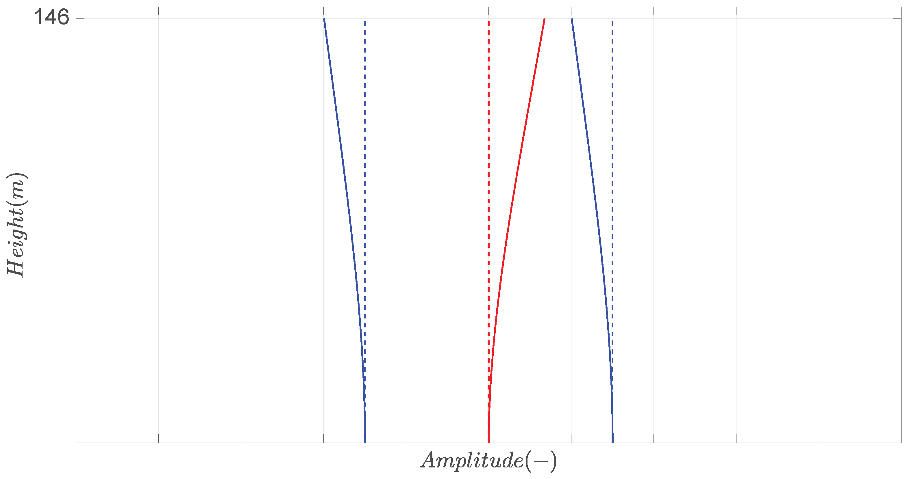
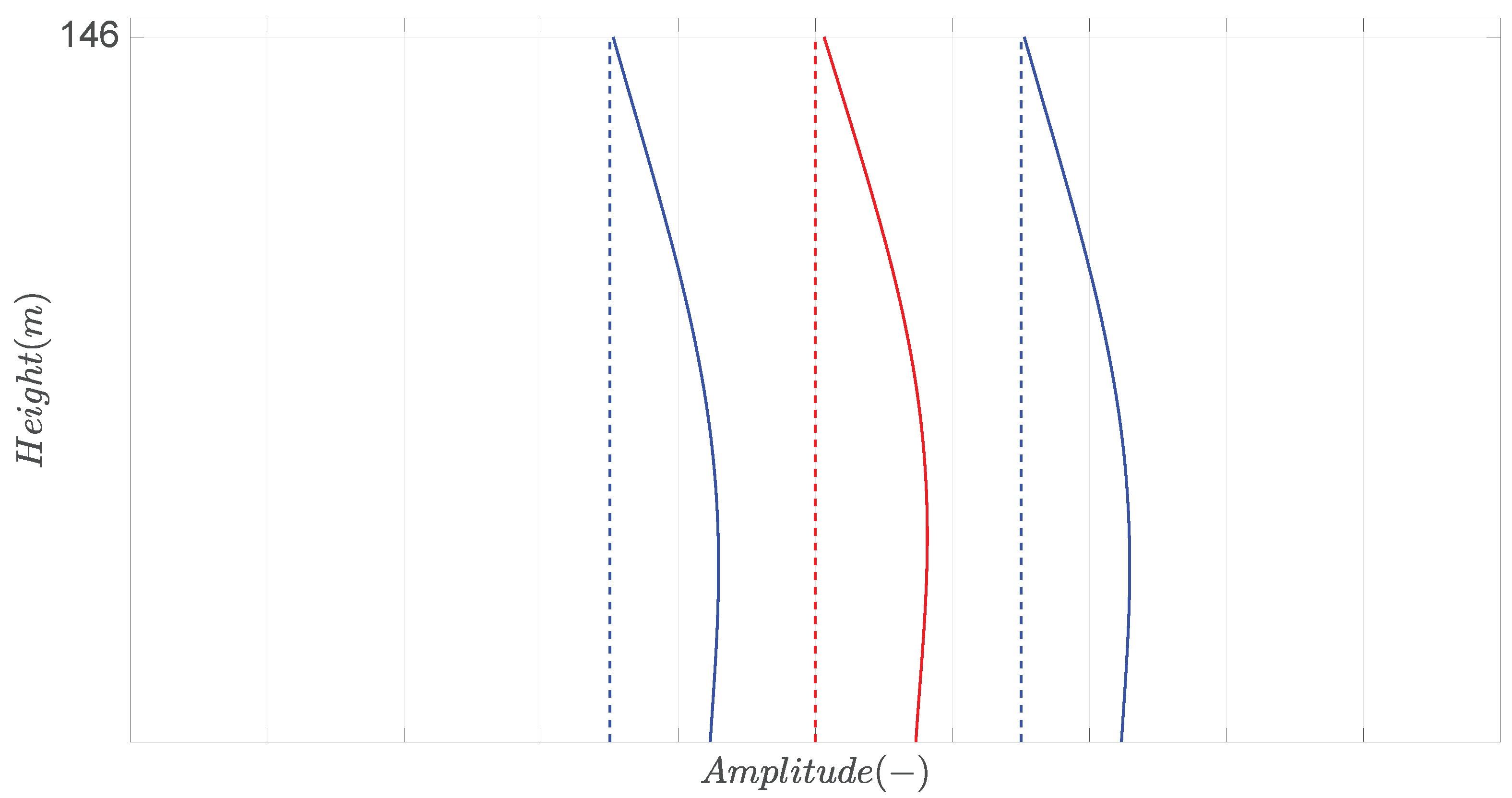
4. Comparison of the Experimental and Modelling Results

The model described above is now used to mimic the response of the JuBi tower subject to wind. To this end, first the parameters of the model are tuned such that the experimentally identified and predicted natural frequencies coincide. The stiffnesses of the soil-foundation ($K_{xx}$ and $K_{\theta \theta }$) are obtained making use of the Dynapile software [13]. The bending stiffnesses of each beam, $E{I}_1$ and $E{I}_2$, and the mass per unit length, $\rho A_1$ and $\rho A_2$, are first estimated based on the provided technical information [14]. Then, the spring stiffness, $K_d$, is tuned in order to find the best frequency match (see

Table 2. Comparison of the experimentally identified and modelled natural frequencies in the weak direction.

Natural Frequencies in the Weak Direction
	Exp.Identified [rad/s]	Model [rad/s]
${\omega }_{n,1}$	2.5	2.5
${\omega }_{n,2}$	2.9	2.9
${\omega }_{n,3}$	10.3	10.3

).

Once the frequencies are matched the dissipation elements are tuned so as to obtain the best match of the resonance peaks height.

Only the response registered by accelerometer 5, corresponding to the weak direction of the buildings, is used for tuning. The resultant best fit is shown in Figure 9.

Figure 9 shows good agreement between the model and the experimental data for the closely spaced modes. Also, a good correspondence for the second bending mode, which is located at the frequency of $\approx 10.3$ rad/s can be seen. The experimentally observed peak at the frequency of $\approx 6$ rad/s corresponds to the torsional mode as shown in Figure 6. Therefore, given that the model does not take into account bending–torsion coupling effects this mode is not captured by the model.

It should be pointed out that the beams in the model represented by Figure 7 are coupled not only through the uniformly distributed visco-elastic elements, but also through the foundation. To determine the influence of the coupling, the following study, of which the results are plotted in Figure 10 and Figure 11 is carried out.

Figure 10 shows the behaviour of the closely spaced resonant frequencies for a broad range of rotation spring stiffness, $K_{\theta \theta }$, values. This figure reveals that from a certain value of the stiffness, the peaks veer away rapidly. This evidences that the coupling is mainly due to the coupling between the beams through the foundation. Figure 11 shows the influence of the uniformly distributed springs, $K_d$, on the closely spaced modes.

The change in the spring stiffness, $K_d$, influences the overall behaviour. However, in this case, the closely spaced modes do not veer away from each other, but both shift along the frequency axis.

Given that, in the case of the studied building, Figure 10 and Figure 11 show that the coupling of the beams takes place mainly through the foundation. When the soil stiffness becomes infinite (fixed base) the coupling through the foundation disappears and the double-peak behvaiour is no longer present. By softening the rotational soil resistance, the coupling between the beams and the foundation becomes stronger, and then the resonant frequencies start veering away from each other until certain value, in which, the soil resistance is so low that first mode becomes unstable. This can be understood in the sense that the complex-valued natural frequency contains only an imaginary part.

It is also of interest for this study to observe to which modal shapes each of the resonant frequencies that were obtained correspond.

Figure 12 and Figure 13 show that the resonant frequencies of the two peaks correspond to very similar vibrational shapes. This underlines the fact that the coupling between the beams is rather weak. Moreover, the mode shape corresponding to the third resonant peak confirms that this frequency corresponds to the second bending mode as can be observed in Figure 14.

It is, therefore, shown that under certain structural complexity, to mimic the dynamic response of a high-rise building it is necessary to take into account the weak coupling between the main structural elements of the building. This should also include the coupling through the foundation.

5. Conclusions

In this paper, a model based on a double-beam system is used to resemble the dynamic behaviour of a high-rise building. The horizontal stability of the studied building is achieved by means of a complex structural system based on three inner cores and outer walls. Given the fact that the cores and the outer walls are connected by the floors and the foundation, a double-peak behaviour corresponding to two closely spaced modes is observed in the experimental results. This is argued to be a consequence of a weak coupling between the core and the walls.

In order to support the above statement a double-beam model is developed (Figure 7), and its predictions are compared to full-scale measurements. The bottom end of the model is constrained by translational and rotational visco-elastic elements that represent the resistance and the capacity of energy dissipation of the soil in the horizontal and rotational directions. The uniformly distributed springs and dashpots represent the coupling between the inner cores and the outer walls. Results of the study carried out in this paper (Figure 10 and Figure 11) show that experimentally observed closely spaced modes are the consequence of the weak coupling between the core and the walls through the foundation.

References

1. Gentile, C.; Poggi, C.; Ruccolo, A.; Vasic, M. Vibration-Based Assessment of the Tensile Force in the Tie-Rods of the Milan Cathedral. Int. J. Archit. Herit. 2019, 13, 411–424. [Google Scholar] [CrossRef]
2. Seelig, J.M.; Hoppmann, W.H. Impact On An Elastically Connected Double-beam System. J. Appl. Mech. 1963, 31, 31. [Google Scholar]
3. Seelig, J.M.; Hoppmann, W.H. Normal mode vibrations of systems of elastically connected parallel bars. J. Acoust. Soc. Am. 1963, 36, 30. [Google Scholar]
4. Dublin, M.; Friedrich, H.R. Forced Responses of Two Elastic Beams Interconnected by Spring-Damper Systems. J. Aeronaut. Sci. 1956, 23, 824–829. [Google Scholar] [CrossRef]
5. Rao, S. Natural vibrations of systems of ellastically conected Timoshenko beams. J. Acoust. Soc. Am. 1974, 55, 1232–1237. [Google Scholar] [CrossRef]
6. Chonan, S. Dynamical Behaviors of Elastically Connected Double-Beam Systems Subjected to an Impulsive Load. Trans. Jpn. Soc. Mech. Eng. 1975, 41, 2815–2824. [Google Scholar] [CrossRef]
7. Hamada, T.R.; Nakayama, H.; Hayashi, K. Free And Forced Vibrations Of Elastically Connected Double-beam Systems. Bull. JSME 1983, 26, 1936–1942. [Google Scholar] [CrossRef] [Green Version]
8. Dougla, B.E.; Yang, J.C.S. Transverse compressional damping in the vibratory response of elastic-viscoelastic- elastic beams. AIAA J. 1978, 16, 925–930. [Google Scholar] [CrossRef]
9. Irie, T.; Yamada, G.; Kobayashi, Y. The steady-state response of an internally damped double-beam system interconnected by several springs. J. Acoust. Soc. Am. 1982, 71, 1155–1162. [Google Scholar] [CrossRef]
10. Vu, H.; Ordoñez, A.; Karnopp, B. Vibration of a double-beam system. J. Sound Vib. 2000, 229, 807–822. [Google Scholar] [CrossRef]
11. Oniszczuk, Z. Damped vibration analysis of an elastically connected complex double-string system. J. Sound Vib. 2003, 264, 253–271. [Google Scholar] [CrossRef]
12. Li, Y.X.; Sun, L.Z. Transverse Vibration of an Undamped Elastically Connected Double-Beam System with Arbitrary Boundary Conditions. J. Eng. Mech. 2015, 142, 04015070. [Google Scholar]
13. Gómez, S.S.; Metrikine, A.V. The Energy Flow Analysis as a Tool for Identification of Damping in Tall Buildings Subjected to Wind: Contributions of the Foundation and the Building Structure. J. Vib. Acoust. 2018, 141, 011013. [Google Scholar] [CrossRef]
14. Sánchez Gómez, S. Energy Flux Method for Identification of Damping in High-Rise Buildings Subject to Wind. Ph.D. Thesis, Delft University of Technology, Delft, The Netherlands, 2019. [Google Scholar]
Figure 1. The JuBi tower.
Buildings 10 00132 g001
Figure 2. The instrumentation configuration at the 9th, 22nd and 37th floors.
Buildings 10 00132 g002
Figure 3. Acceleration response of the building at the 37th floor.
Buildings 10 00132 g003
Figure 4. Response of accelerometer 5 versus accelerometer 6.
Buildings 10 00132 g004
Figure 5. Power spectral density (PSD) functions of sensors at the 37th floor.
Buildings 10 00132 g005
Figure 6. PSD functions of the shifted signals at the 37th floor.
Buildings 10 00132 g006
Figure 7. Model of a high-rise building with a double-beam system connected by uniformly distributed visco-elastic elements.
Buildings 10 00132 g007
Figure 8. Best fit of the spectral density function of the wind force to the exponential function shown in Equation (15) at three different heights.
Buildings 10 00132 g008
Figure 9. Comparison of the modelling with the experimentally identified power spectral density.
Buildings 10 00132 g009
Figure 10. Influence in the natural frequency due to the foundation coupling.
Buildings 10 00132 g010
Figure 11. Influence in the natural frequency due to the spring coupling.
Buildings 10 00132 g011
Figure 12. Mode shape corresponding to the first vibrational mode ( 2.5 rad/s) obtained from the model.
Buildings 10 00132 g012
Figure 13. Mode shape corresponding to the second vibrational mode ( 2.9 rad/s) obtained from the model.
Buildings 10 00132 g013
Figure 14. Mode shape corresponding to the third vibrational mode ( 10.3 rad/s) obtained from the model.
Buildings 10 00132 g014