Abstract
The effectiveness of Double Concave Curved Surface Sliders (DCCSS), which initially spread under the name of Double Friction Pendulum (DFP) isolators, was already widely proven by numerous experimental campaigns carried out worldwide. However, many aspects concerning their dynamical behavior still need to be clarified and some details still require improvement and optimization. In particular, due to the boundary geometrical conditions, sliding along the coupled surfaces may not be compliant, where this adjective is adopted to indicate an even distribution of stresses and sliding contact. On the contrary, during an earthquake, the fulfillment of geometrical compatibility between the constitutive bodies naturally gives rise to a very peculiar dynamic behavior, composed of continuous alternation of sticking and slipping phases. Such behavior yields a temporary and cyclic change of topology. Since the constitutive elements can be modelled as rigid bodies, both approaches, namely Compliant Sliding and Stick-Slip, can be numerically modelled by means of techniques typically adopted for multi-body mechanical systems. With the objective of contributing to the understanding and further improvement of this technology, a topology-changing multi-body mechanical model was developed to simulate the DCCSS. In the present work, attention is focused on details regarding geometrical compatibility and kinematics, while the complete dynamics is presented in another work. In particular, for the sake of comparison, the kinematic equations are presented and applied not only for the proposed Stick-Slip approach, but also for the currently accepted Compliant Sliding approach. The main findings are presented and discussed.
1. Introduction
Friction pendulum devices, since their early introduction [1], have earned increasing attention as a valid alternative to elastomeric bearings, for the seismic protection of both low to medium-rise buildings, and bridges. The resulting relevant scientific research ranges from early studies on the friction properties of the kinematic pair, mainly composed so far of polytetrafluoroethylene (PTFE) and stainless steel (e.g., [2,3]), to the proposal of many prototypes and their mechanical modelling (e.g., [3,4,5,6,7,8]), and up to the study of the overall behavior of an isolated structure (e.g., [9,10,11]). More recently, the relevant scientific output has encompassed both rigorous analytical–numerical studies (e.g., [12,13,14,15,16,17,18,19]), and experimental tests (e.g., [20,21,22,23]). Such devices are based on the principle of obtaining the decoupling between the movement of the structure and the underlying ground by means of the relative sliding between coupled spherical surfaces, one of which is in plain polished stainless steel and the other coated by a particular material chosen to ensure a suitable value of the friction coefficient. The spherical shape of the two surfaces forming a kinematic pair is supposedly necessary in order to provide the device with self-recentering capability. The simplest of such devices envisages the presence of one only of these spherical kinematic pairs even though proposals of prototypes with multiple sliding surfaces can be found both in the literature and on the market (e.g., [8]). The larger the number of coupling surfaces composing the device, the more difficult the prediction of its mechanical behavior during an earthquake appears to be. In the present work, attention is focused on the so-called double friction pendulum (DFP) device (Figure 1).
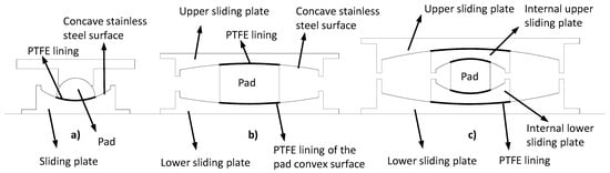
Figure 1.
Friction pendulum bearings: (a) single (SFP), (b) double (DFP), and (c) so-called triple friction pendulum (TFP). PTFE stands for polytetrafluoroethylene.
One of the aspects that has been largely investigated is the mathematical model of the horizontal force–displacement hysteretic curve, which needs to be implemented in the finite element models (FEM) of isolated structures in order to carry out the dynamic analyses.
Complex tribological (i.e., friction-related) systems are known to be susceptible to (1) stick-slip and (2) sprag-slip phenomena (e.g., [24]). Where the former consists of the likely alternation of time intervals of sliding to time intervals of absence of sliding, while the latter consists of vibrations that may activate in the direction orthogonal to the sliding one. In this scenario, many questions arise about the actual functioning of these devices. It is evident that the topic is complex and needs to be faced from a multidisciplinary standpoint, also involving mechanical and tribological engineering expertise (e.g., [25,26,27,28]).
Attention was initially devoted to studying the order of magnitude of the temperature rises that can take place in these devices during an earthquake, and their influence on the tribological aspects. For this reason, a pseudo-static thermomechanical model was developed [29] to simulate the results of experimental tests retrieved in the literature, in terms of both temperature rises and force–displacement hysteretic curves. From this point on, we have started analyzing how the geometrical compatibility of these devices could be fulfilled [30] and we realized that due to geometrical compatibility fulfillment, the mechanical behavior may be characterized by a continuous alternation of sticking and slipping phases, with contextual lifting of the base-isolated mass, as described hereinafter. Subsequently [31,32,33], we have been working on the development of a numerical strategy to simulate the dynamical behavior of a DFP.
Provided that the DFP can be seen as an assemblage of rigid bodies supposedly sliding with respect to each other, the urge to rapidly develop a numerical model to simulate the DFP devices initially led us to undertake the so-called Embedded numerical-modelling technique [27], which leads to a minimum number of solving equations [31]. That strategy, which led to a number of equations equal to the number of independent kinematic variables, turned out to be impracticable since the minimum number of equations is strongly coupled and difficult to solve. Subsequently, the solving equations have been written [33] by means of the so-called Augmented Formulation technique [26,27], which is a technique that yields a system of Differential and Algebraic Equations (DAE). Though the number of solving equations is equal to the sum of both independent and dependent kinematic variables plus the number of constraint reactions, the resulting DAE system can be more easily implemented, and solved, by means of consolidated numerical techniques (e.g., [34]).
After having singled out the most suitable numerical strategy to model the dynamic behavior of these devices, the decision was made to apply it not only to simulate the envisioned mode of behavior herein proposed, but also the one currently accepted. Where the former envisages that the relative movement undergone by the numerous rigid bodies constituting the device is composed of a continuous alternation of stick and slip, the latter assumes that a pendulum-like behavior can be clearly identified, with contextual compliant sliding occurring along the coupled surfaces.
In particular, in this work, before describing in detail the envisioned mode of behavior and the corresponding multi-body kinematics, two steps backwards have been taken. In fact, in the first part of the paper, some considerations are presented about the count of the degrees of freedom, as a function of the kinematic constraints, in order to understand if, in the case of DFPs applied underneath a building, the alleged pendulum behavior can actually be expected. In the second part of the paper, the multi-body kinematics equations are written and applied, taking the assumptions of pendulum-like behavior and relative compliant sliding for granted. This is in order to try to understand initially if the solution is numerically possible, and then if, in the obtained results, something can be singled out that would rather induce one to doubt the validity of the underlying assumptions and to deem the assumption of the stick-slip behavior herein proposed more probable. In particular, the obtained equations are applied to two prototypes of DFP.
In the third part of the paper, the genesis of the mode of behavior proposed for the DFPs is presented along with the main features.
In the fourth part of the paper, the multi-body kinematics equations are then written and applied assuming that the behavior of such devices is not of the pendulum type, with compliant sliding, but rather of the stick-slip type. The obtained equations are applied to the same two prototypes and the results are compared with those obtained previously, in search for confirmations about the validity of the envisioned mode of behavior proposed.
2. Research Motivation: Can We Always Speak about Pendulum?
Interest in quantifying the effects of earthquake-induced temperature rises on the effectiveness of friction pendulum devices initially brought to the development of a simple pseudo-static thermomechanical model [29]. That model meant to simulate the experimental results retrieved in the literature by reproducing, for an imposed displacement time history, both temperature rises and force–displacement hysteresis curves. When that model was applied to simulate the relatively high velocity pseudo-static tests (), regardless of the number of pendula, the agreement between numerical and experimental hysteretic curves was satisfactory. On the contrary, when the low velocity tests were simulated, in particular for some tested TFP prototypes, in order for the agreement between numerical and experimental curves to be satisfactory, it was necessary to introduce, stepwise, a fictitious force whose physical meaning was not clear. Decomposing a posteriori the overall hysteretic curve in the curves of the single sliding kinematic pairs, it was found that the curves at the interfaces between the pad and the external plates showed an initial increase in horizontal force at motion reversal. Among other things, such behavior had already been observed experimentally [5]. However, doubt arose that such behavior might be due to a velocity-related sticking. This finding has stimulated the authors to carry on with the investigation in order to understand the actual functioning of these devices, which is very simple only apparently. Each of such devices is composed of an assemblage of rigid bodies and, regardless of the number of coupled sliding surfaces, must be characterized by at least one degree of freedom, in order to function as a mechanism.
If we consider a single pendulum (Figure 2a), this will actually be a mechanism, with spherical sliding surface effectively constituting a compliant kinematic pair, which means with an even distribution of contact stresses, if it is made as depicted in Figure 2a. This is composed of three rigid bodies (RBs) that are: (1) the concave lower plate (RB1), which is fixed to the global inertial system, with a number of constraints equal to 3, (2) the element RB2, coupled with the lower plate by a convex sliding surface of the same radius, which is fixed () to the third RB3, (3) which is the connecting rod, constrained to the global inertia system by means of a pinpoint (). In this case, since RB1 is fixed, other internal kinematic constraints are not needed to guarantee compliant contact between the two sliding surfaces and the whole system is actually a mechanism, having: (a) nine global coordinates (), (b) eight kinematic constraints, and consequently, (c) one degree of freedom (). If the horizontal translational constraint on RB1 is removed, thus admitting that it can be moved by the earthquake, in order for the compliant coupling between the concave (RB1) and the convex surface (RB2) to be maintained, it is necessary to introduce another two internal kinematic constraints (Figure 2b) as will be further clarified hereafter. However, in this case, the device is no longer a mechanism, since the number of constraints is equal to the number of global coordinates, and the device, thus statically determinate, does not move at all. For the multi-body system to go back to being a mechanism, it is thus necessary to remove one constraint. For instance, the vertical translational constraint on the pivot point of RB3 may be removed, leaving only the horizontal translational one, which may be modelled, as usually performed for fixed-base buildings, by a viscous damper that also simulates the resistance opposed by the air to the horizontal deformation of the building (Figure 2c). In this case, the hinge around which RB3 may rotate, can also move vertically, and therefore, the total number of constraints is and the system has 1 degree of freedom. In this scenario, it is natural to wonder what happens for a squat, rigid-body-like building supported by the so-called DFP bearings (Figure 2d). Given the observations made so far for the single pendulum, the situation must be more complex. Attention has been focused on the DFP for a two-fold reason: (1) the single pendulum can be seen as one of its simplifications, and (2) it also constitutes the internal nucleus of the triple (Figure 1), so that the advantages brought by the understanding of its behavior are manifold.
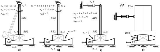
Figure 2.
Degrees of freedom of some examples of multi-body assemblages: (a) pendulum or compliant kinematic pair, (b) pendulum with translating base, (c) pendulum with translating base (horizontally) and pivotal point (vertically), (d) squat building (not in scale) isolated with DFP (DCSSD).
3. Supposed Compliant Sliding
In compliance with both the Italian Building Code [35] and EuroCode8 [36], when DFP devices are installed under a building, they must be placed in between two rigid diaphragms in order to impose the same horizontal movement to each of them. Such diaphragms are realized with grids of Reinforced Concrete (RC) beams, usually completed by a slab, also in RC. Each of these RC beams’ grids also has a not negligible out-of-plane flexural stiffness. Due to this and to the collaboration of the hyperstatic superstructure, the DFPs are forced to deform, during an earthquake, with the predominant horizontal component, with the upper and lower bases that move remaining horizontal. In this way, any rotation of the upper and lower plate is avoided.
3.1. Numerical Details
The DFP can be assumed as composed of three rigid bodies (RB), which are: (a) rigid bodies 1 (RB1) and 3 (RB3), schematizing the lower and upper sliding plate, respectively, and (b) rigid body 2 (RB2) schematizing the internal pad (Figure 3). It is reasonable, at least for the time being, to assume the total absence of any deformation. In this case, the position of each i-th rigid body RBi in the global Cartesian reference system is identified by three generalized coordinates, which are: the coordinates and of its centroid , and the rotation of its local reference system with respect to the global abscissa axis (Figure 3). The rotation angle is assumed counterclockwise with respect to the positive verse of the axis . Using the three coordinates and , the position of each j-th point belonging to the generic i-th RBi has coordinates, in the global Cartesian reference system, given as follows:
where:
is the position vector of the arbitrary point defined in the RB’s local coordinate system, and is the transformation matrix from the body’s coordinate system to the global coordinate system defined in terms of the rotation angle , as follows:
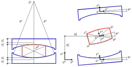
Figure 3.
Double friction pendulum device as an assemblage of rigid bodies: geometric quantities and generalized coordinates.
The coordinates and are referred to as the absolute Cartesian generalized coordinates of RBi. Thus, the multi-body schematizing the DFP, consisting of three RBs, has nine independent generalized coordinates. The vector of the generalized coordinates of the DFP multi-body system is then defined as:
According to the currently accepted theory about the behavior of such devices, sliding is expected to occur along the two kinematic pairs composed of: (1) the concave surface of RB1 and the coupling convex lower base of RB2, and (2) the concave surface of RB3 and the coupling convex upper base of RB2. How would the corresponding kinematic constraint equations be written in order to model such expected behavior? It is necessary to impose that two points of each of the convex surfaces of RB2 are constrained to move on the relevant coupled concave surface of either RB1 or RB3. In fact, if we imposed one constraint only, for instance on to move along a circumference concentric to , it would not suffice, since RB could still undergo some rotation (Figure 4a). Moreover, even if we imposed one constraint on a point belonging to the convex surface of RB2, vertex for instance, to move along , RB2 could still rotate (Figure 4b). Ultimately, the only way to impose that RB2 actually slides along the concave surface is to impose such constraint on at least two points of its convex surface (Figure 4c).
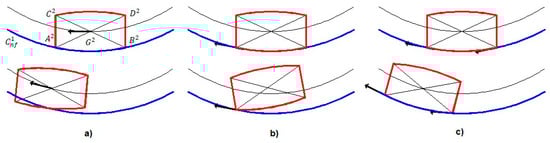
Figure 4.
Alternative kinematic constraints solutions: (a) centroid has to migrate along a circle concentric to the concave surface , (b) the pad vertex has to migrate along , (c) both vertices and have to move along .
In order to uncouple the superstructure from the ground shaking, these devices must undergo some overall deformation, that is, some internal relative movement between the constitutive components. This means that, overall, the multi-body system must be statically underdetermined in order to be a mechanism. Thus, it must have at least one degree of freedom, which means at least one generalized coordinate must not be constrained.
According to most testing protocols (e.g., [23,37]), a DFP is tested using a machine that only allows vertical translation to the upper plate and imposes, generally by a vibrating table, a kinematic history of displacement and velocities on the lower plate (Figure 5). In such conditions, the non-linear kinematic constraint equations, assembled in matrix format, are written as follows:
where the first constraint equation imposes a displacement history on the translational horizontal generalized coordinate of the lower plate, which is indicated as RB1. The second and third constraint equations impose null vertical translation and rotation, respectively, for RB1. The kinematic constraint equations from the fourth to the seventh impose sliding to take place at the corner points of the two convex surfaces of the RB2 schematizing the pad. In particular, each of them imposes that the vector that describes the relative movement of generic point (actually, one of the four points , , , ) with respect to its position , at the previous time step , along the coupled concave surface (), is tangent to the spherical surface itself. This is expressed imposing that the projection of vector along the versor of the normal to in is null. In fact, the fourth kinematic constraint equation is written as:
meaning that the vector of the components of the displacement of point , belonging to RB2 in the global inertial Cartesian system, and with respect to its previous position occupied on RB1, namely along the surface , has a null component along the versor of the normal to in —the expression for the latter is determined as follows:
in which and are the global position vectors of the center of and position , respectively, as points belonging to RB1.
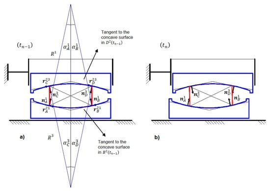
Figure 5.
Constrained model of the DFP to simulate the experimental tests, assuming that compliant sliding occurs: (a) starting configuration, and (b) displaced configuration.
With these premises, the fourth to seventh non-linear kinematic equations are written as follows:
where , , , and are the local position vectors of points and , and and , along the circumferences and , respectively, at time ; , , , and are the angles defining the current local position of RB2 vertices along the two circumferences and (Figure 5), and and are the constant quantities characterizing the geometry of RB2, given by:
in which is the diagonal and is the opening angle of the pad, respectively (Figure 3). The eighth and ninth constraint equations impose that RB3, schematizing the upper sliding plate, can undergo neither horizontal translation nor rotation.
Due to the high non-linearity of the kinematic constraint equations in terms of the generalized coordinates, they are often solved by means of the Newton–Raphson algorithm (e.g., [26,27]). This iterative procedure starts by making an estimate of the desired solution vector. If this estimate at a certain instant is denoted as , the exact solution can be written as . By using Taylor’s theorem, and neglecting the higher order terms, the kinematic constraint equations become:
where is the vector of Newton differences and is the constraint Jacobian matrix, whose j-th row is defined as follows:
In this case, the system is kinematically driven since the number of constraint equations is equal to the number of generalized coordinates and, if the constraints are linearly independent, must be non-singular and invertible. In this case, Equation (13) can be solved for the vector of Newton Differences and this vector can be used to iteratively update the vector of the system’s generalized coordinates as follows:
With these premises, the assumed compliant sliding can actually take place along the two concave surfaces only if the constraint Jacobian matrix is non-singular and invertible, which means that the determinant is non-null.
For the multi-body model (hypothesis of compliant sliding) herein described (Figure 5), all the terms of the Jacobian matrix are null except for the following ones:
where the generic term indicates the partial derivative of the i-th constraint equation with respect to the j-th multi-body generalized coordinate of Equation (4).
With these equations, the determinant of the constraint Jacobian matrix becomes:
where all addends are generally different than zero so that itself is generally different than zero and results non-singular and invertible; thus, sliding can actually occur along the two surfaces. In the case of the previous time step characterized by symmetric rest position , Equation (29) becomes:
which, again, is generally non-null since it may vanish only if either , , or but none of these can be possible.
However, even if the model described so far admits a numerical solution, when looking more closely at the trajectory undergone by the corner points of RB2 (Figure 6), one realizes that such relative movement would actually yield interpenetration of matter, which would imply some wear that is not reported in experimental testing.
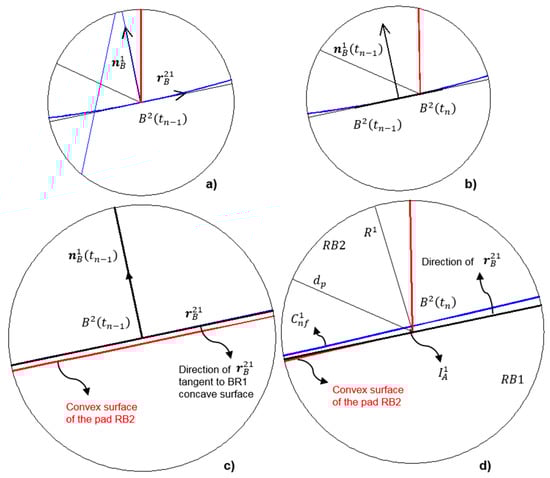
Figure 6.
Constrained (Compliant Sliding) model of the DFP to simulate the experimental tests: details of the (a) undisplaced and (b) displaced configuration, (c,d) zoom of the displaced configuration.
Moreover, in order to avoid such interpenetration of matter, we should impose four other linear kinematic constraints at the corner points of the convex surfaces of RB2 to force these points to move along circumferences instead of tangent straight lines, resulting in a statically indeterminate multi-body assemblage. However, such an assemblage would not be a mechanism any longer, due to this static indeterminateness. Thus, what is the real relative movement undergone by the numerous rigid bodies constituting the DFP during an experimental test and, more generally, during an earthquake? Let us start by analyzing the results of the model complying with the alleged kinematical behavior, in terms of only displacements and their instantaneous increments (velocities), neglecting accelerations and forces for the time being. Two DFP prototypes are analyzed, whose geometrical features and testing parameters are listed in Table 1. The former include (Figure 3): , height and thickness of the retaining ring; , radius and opening angle of the concave surface; height of the straight cylinder part of the RB2; and opening angles defining the dimensions of the convex bases of RB2, coupled with RB1 and RB3, respectively. The testing parameters include: initial value of ground-imposed displacement; maximum value and circular frequency of the ground-imposed displacement time history; initial rotation of RB1 and RB2, respectively; time extent and time increment of the ground-imposed time history .

Table 1.
Analyzed DFP prototypes: values for the input parameters adopted in the analyses.
3.2. Results: The First Time-Step t1 of Sliding
In accordance with what has been pointed out in the previous paragraph, an aspect that is undoubtedly interesting to analyze is the amount of interpenetration of matter at the corners of the pad, namely RB2. The interpenetration at each of the corners of RB2, which are the points , , , and , can be measured along the radial straight lines passing through themselves and the centers of the concave surfaces, yielding , , , and , respectively (Figure 6). It is interesting to start by evaluating the interpenetration at the initial instant of sliding: (a) starting from different geometrical configurations, which are herein singled out simply by the relevant value of , (b) for two different values of ground-imposed displacement , and (c) for two different prototypes of double friction pendulum bearings, herein labelled as DFP1 and DFP2. The geometrical characteristics of these latter are listed in Table 1. The main difference between the two is that the pad of DFP1 has a more flattened and lenticular shape, while the pad of DFP2 is squatter. The values of incremental ground-imposed displacement taken into consideration are 5 and 10 cm. These values should indeed be assumed coherently with the ground-motion velocity, but they are herein intentionally assumed slightly larger in order to investigate their numerical influence on the value of the initial interpenetration at .
As can be gathered from Figure 7, the value of the initial interpenetration for each of the vertices of the pad almost doubles by doubling the imposed ground displacement, from 5 to 10 cm, independently of the analyzed DFP prototype and regardless of the value of . What is more interesting to observe is that for both analyzed prototypes, the interpenetration evaluated at the two endpoints of each diagonal (e.g., and ) assumes exactly the same value, for whatever value of the initial rotation of RB2, so that the two relevant curves result superimposed to each other. Moreover, the initial interpenetration at the endpoints of one diagonal of RB2 is always larger than at the endpoints of the other diagonal (Figure 7). This, in the context of the model herein applied, which assumes the various components to be rigid bodies, thus impenetrable, means that in the points with higher interpenetration, there would actually be a larger concentration of stresses so that the pad (RB2) would work essentially, or to a larger extent, on one diagonal (e.g., the one singled out by vertices and ). Such deduction would be legitimate even if the assumption of infinitely rigid bodies were removed and the constitutive bodies were considered as deformable. Such effect is more pronounced for the prototype with the squatter pad (DFP2) and for initial configurations characterized by a larger value of in the absolute value, which corresponds, being negative in the contemplated cases, to a clockwise rotation of RB2 (compare Figure 3). In fact, as can be gathered from Figure 7a,b, the initial interpenetration at the endpoints of the diagonal is on average larger than that calculated at the endpoints of the diagonal , approximately of for and of for . These differences might seem tiny, but they would yield stress differences that may not be negligible, if the elastic modulus of the constitutive material were taken into account [37]. The difference in value between the interpenetration calculated at the endpoints of the diagonal and that at the endpoints of the diagonal is more pronounced for the prototype with the squatter pad (Figure 7c,d). In fact, such difference reaches a maximum value of approximately for and of for . Note however that, in general, the initial interpenetration tends to increase by increasing the global deformation of the device (characterized by larger values of ), with respect to the undeformed configuration at rest (). This is due to the fact that, for the reasons already explained in a previous paragraph, the upper and lower plates are constrained to translate while remaining horizontal. In Figure 7, the values of the determinant of the constraint Jacobian matrix are also plotted, as an example, for the cases herein examined. These values result, as expected, generally different than zero, meaning that a numerical solution actually exists.
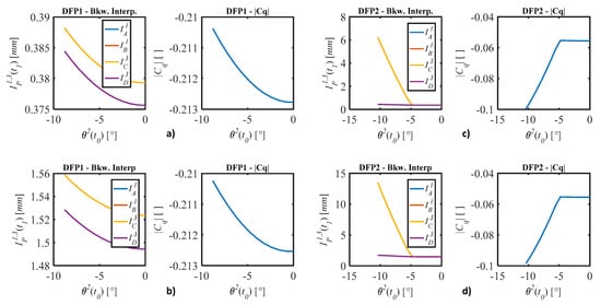
Figure 7.
Interpenetration at the initial sliding time step for the RB2 corners and determinant for different initial configurations for DFP1 (a,b) and for DFP2 (c,d), with (above) and with (below).
In the case of the DFP1 prototype, the more flattened one, the difference in initial interpenetration is less pronounced than for DFP2, but is always present, indicating that according to this model, initial sliding concentrates on the endpoints of one of the two diagonals of the pad. The device would not start sliding with an evenly distributed interpenetration along the two kinematic pairs but, conversely, on the two vertices of a single diagonal. This can also be gathered from Figure 8a, in which the displaced configuration of DFP1 is plotted, for initial geometrical configuration characterized by and imposed displacement of . Thus, a more flattened shape of the pad yields, according to this model, and reasoning only in terms of displacement kinematics, a relatively more evenly distributed initial interpenetration, even if the value at the vertices of one diagonal is slightly larger than at the others. This one-diagonal effect is more pronounced for the DFP2 prototype, as can be gathered from Figure 8b, in which the displaced configuration is plotted for the initial and imposed displacement of . It must be stressed that if sliding effectively took place according to this compliant sliding model, stresses would concentrate at the endpoints of the diagonal opposite to the one that, taking into consideration the elastic deformations of the pad, are consequent to a rightward imposed movement . In fact, in such case (compare Figure 8), the most stressed diagonal of RB2 would be the compressed one, which is , instead.
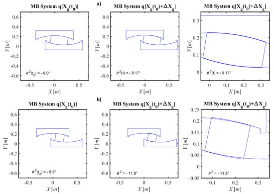
Figure 8.
Initial and deformed configurations corresponding to breakaway interpenetration: (a) DFP1 prototype with , and (b) DFP2 with .
3.3. Results: The Time Histories
For the two prototype DFPs, whose characteristics are listed in Table 1, the time history response to an earthquake-like sinusoidal ground movement was also evaluated. The values assumed for maximum imposed displacement and circular frequency are listed in Table 1.
As can be gathered from Figure 9, for the DFP1 prototype, for both integration time steps of 0.01 and 0.001 s, the curves representing the time histories of corner interpenetration are almost superimposed to each other even if in the former case, in correspondence of the peaks, those curves slightly diverge from each other. Even though this would induce the conclusion that the DFP slides in a compliant form, when interpenetration is considered in relative terms, meaning in terms of the difference between interpenetration at the RB2 corners that are supposed to slide along the same concave surface (i.e., and ), it can be realized that sliding concentrates at the extremities of one diagonal only. In fact, as can be gathered from Figure 10, regardless of the integration time step value, the time histories of and show a cyclic trend and always have the same absolute value and sign, meaning that interpenetration is systematically and alternatively larger, even though of a slight amount, at the ends of one diagonal only. For the second prototype DFP2, characterized by a squatter pad, the curves representing the time histories of corner interpenetration are superimposed to each other, in pairs, throughout the earthquake-induced displacement history (Figure 9). Moreover, the larger values of interpenetration, in absolute terms, are recorded for the larger integration time step and interpenetration is cyclically concentrated at the ends of one diagonal only. The one diagonal-concentrated interpenetration effect is more evident with larger absolute values than in the case of the more flattened prototype. In fact, the maximum values of difference in interpenetration are equal to approximately 1.6 and 0.18 mm for the integration time steps of 0.01 and 0.001 s respectively (Figure 9), while for DFP1, such values were of the order of and (Figure 10).
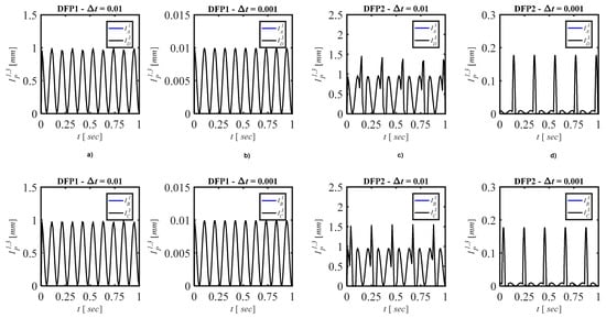
Figure 9.
Time histories of interpenetration at the corners of RB2, for DFP1 and DFP2, at the extremities of diagonal (above) and (below): (a,b) curves for DFP1 and and , respectively, and (c,d) curves for DFP2 and and , respectively.
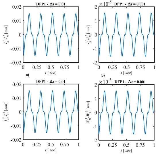
Figure 10.
Time histories of the difference of interpenetration at the corners of the pad supposed to slide along the same concave surface, (above) and for (below), for DFP1: for integration time step (a) , and (b) .
As examples, in Figure 11 and Figure 12, the time histories are plotted of (a) imposed ground displacement and velocity , and (b) global coordinates and , where the latter are the pad rotation and the upper plate vertical motion, respectively. In the same figures, the initial and final computed configurations are also plotted. Figure 11 refers to the analysis of the DFP1 with integration time step of 0.01 s and Figure 12 to the DFP2, with integration time step of 0.001 s. Note that the maximum value of imposed ground displacement was evaluated as the one corresponding to the maximum geometrical capacity of the given prototype, because any other exceedance would result in a rigid body translation of the device, with the internal pad leant against the relevant retainer. For the DFP1, for imposed ground motion characterized by and , maximum and residual rotation are and , respectively, while the maximum upward movement, with respect to the initial rest position, is and the residual is (Figure 11). For the DFP2, for imposed ground motion characterized by and , maximum and residual rotation are and , respectively, while the maximum upward movement, with respect to the initial rest position is and the residual is (Figure 12). By comparing Figure 9, Figure 10 and Figure 11, it can be noticed that the peak values of difference of interpenetration at the extremities of the two diagonals (i.e., and ) are cyclically attained in correspondence of the maximum relative values of ground velocity. This is simply due to the fact that for a constant value of the integration time step , the maximum instantaneous values of imposed displacement increments are attained for the maximum values of velocity, being .
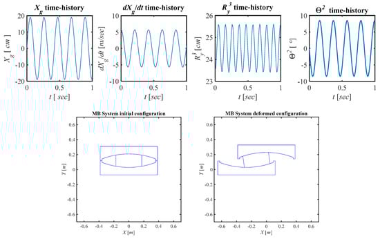
Figure 11.
Time histories of imposed ground displacement and velocity and global coordinates and for DFP1 and for integration time step (above), and relevant initial and final deformations (below).
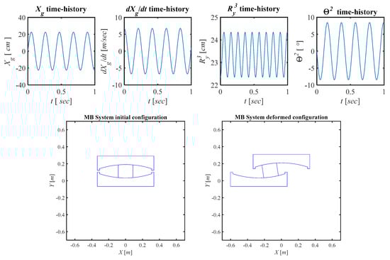
Figure 12.
Time histories of imposed ground displacement and velocity and global coordinates for DFP2 and for integration time step (above), and relevant initial and final deformations (below).
4. Inspiring Physical Observation
In chronological order, before developing and implementing the model described in the previous paragraph, and reflecting on the findings described in paragraph 2, the observation described in the following was made. Suppose a kind of double flat friction bearing (Figure 13), composed of (a) two rigid horizontal steel plates and (b) a rigid steel cylinder placed in between. Imagine that this device is loaded by a vertical force and that friction at the two interfaces is governed by the Coulomb constitutive law (Figure 13b), with a rigid perfectly plastic dependence of the friction force on the relative displacement , and threshold value . Imagine also that the friction coefficient at those interfaces has the same value. If we impose a displacement on the lower plate, due to the rigid plastic constitutive law of interfacial friction, we would immediately have, even for infinitesimally small values of imposed displacement, the mobilization of the friction threshold at each interface. Those two horizontal forces, equal in magnitude and opposite in direction, do generate a couple, to which corresponds a moment that, in the initial configuration, is not balanced by any other couple. That moment would tend to overturn the pad by making it rotate around one of the corners. In such tentative rotation, the points of application of the vertical force would migrate to the pad corners still in contact with the relevant horizontal plates. In this way, even the vertical force would give rise to a couple , opposed to the overturning one and larger in absolute value that would make the pad undergo both a rigid body rotation around its centroid and a simultaneous vertical translation. During such movement of the pad, the diagonally opposed corners, loaded by , would also undergo sliding, up to the new, restored equilibrium configuration (Figure 13e). It is the vertical weight force that restores the geometric compatibility at each time step.
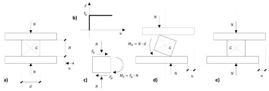
Figure 13.
Case of a flat double friction bearing: (a) undeformed initial configuration, (b) friction’s Coulomb constitutive law, (c) pad free body diagram, (d) intermediate deformed configuration, and (e) final configuration of the whole device.
Geometrical Compatibility
The observation initially made for the case of a double flat sliding isolator can be extended to the double concave one, as follows. The considerations herein presented are based on the following assumptions: the various parts constituting the friction pendulum devices are considered as rigid bodies, thus neglecting, at least for the time being, any possible deformation. In this way, geometrical compatibility is fulfilled each time the two spherical caps constituting the two mating surfaces of a given interface are perfectly superimposed to each other.
The first and most important constraint is represented by the fact that the two outermost horizontal surfaces, lower and upper, can undergo a rigid body motion remaining horizontal, which means that they can only translate remaining parallel to themselves (see paragraph 3). This is due to the fact that, at the extrados of the so-called isolation layer, the various isolators are connected by a rigid diaphragm (e.g., [36]) while, at the intrados, they are by the presence of the foundations structure, which can actually be seen as another rigid diaphragm. In order for that condition to be fulfilled, it is necessary that sliding simultaneously occurs at the two sliding interfaces. For this reason, the friction coefficient should be the same along the two surfaces of the two sliding pairs, i.e., . It is preferable to start by analyzing the behavior of a double friction pendulum in a radial plane, which means in the case of unidirectional imposed horizontal displacement (Figure 14). At a generic time step , the internal deformation undergone, as a function of the imposed displacement by the numerous elements constituting the device, can be decomposed into two subsequent phases. When starting from the rest position (Figure 14a), in the first phase, which means during the first part of the time increment , the pad, due to the imposed displacement , rigidly rotates around one of the lowermost corners () and such rotation also yields a certain vertical displacement of the upper plate. During the second phase of the current time increment , the pad undergoes a rigid rotation around its centroid with the latter simultaneously rigidly translating along the straight line connecting the centers of the two spherical surfaces . This latter direction, resulting from the end of the previous sub-interval , is inclined, with respect to the vertical direction, at an angle of , which is the geometrical parameter accounting for the final configuration assumed by the entire device. The same two-step deformation can be recognized if, at a generic time step , the ground imposes a reversed displacement, and starting from a generic deformed configuration (Figure 14b). The only difference, in the case of reversal, is that initial rigid rotation () involves the other diagonal of the pad (i.e., instead of ). During the second phase, sliding occurs along the corners of the involved diagonal of the pad, and friction is mobilized therein.
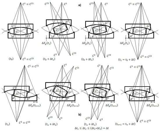
Figure 14.
Case of a DFP device subjected to a horizontal ground displacement contained in a radial plane: (a) rightward ground movement starting from a rest position, and (b) leftward movement starting from a capacity deformation.
The same two-step deformation at a generic instant can be singled out when a more general situation is considered, in which we assume that (1) the pad is already dislocated () from the equilibrium configuration, and (2) the ground-imposed displacement is generically oriented with respect to the global reference system [30]. Even though already dislocated at the start () of the current incremental time step, the pad must have restored, according to the two-step deformation above, a geometrically compatible configuration (Figure 15a). Such displaced configuration, uniquely identified by the two spherical coordinates and , which are the polar and azimuthal angle, respectively (Figure 15), is thus characterized by the fact that the pad axis is superimposed on the segment connecting the two centers of the external spherical surfaces.
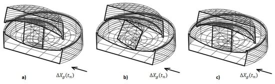
Figure 15.
3D representation of a DFP device subjected to a horizontal ground displacement generically oriented with the pad already dislocated from the initial equilibrium configuration: (a) initial geometrically compatible configuration, (b) sticking along diagonal , and (c) final configuration, after slipping.
Whatever the orientation of the imposed displacement in , it is always possible to single out a plane passing through that displacement orientation and the two centers of the spherical surfaces (one is sufficient indeed, provided that the geometrical compatibility was fulfilled). The geometrically compatible two-step deformation takes place in the plane that, since passing through the spheres’ centers, sections the latter along two circles with maximum radius, i.e., and , herein assumed equal. The two-step deformation is again composed of (1) a rigid body rotation along one of the corners of the pad (which means a point, in 3D), contained in the plane , and (2) a subsequent simultaneous rigid rotation and translation of the pad, always contained in , that restores compatibility (Figure 15). During the second phase (), sliding occurs, simultaneously to the rigid roto-translation, along the corners of the pad. When geometrical compatibility is restored, spherical coordinates assume updated values (Figure 15c).
5. Proposed Stick-Slip Modelling Strategy
The same theory of kinematics of multi-body systems already applied, assuming that the hypothesis of compliant sliding is valid (Paragraph 3), can be applied in the case in which we assume that the mechanical behavior of the DFPs is characterized by the alternation of Stick and Slip phases. Even in this case, the non-linear kinematic equations are written assuming to test one such DFP, by constraining the upper plate (RB3) so that it can only translate vertically and by imposing to the lower plate (RB1) a kinematic history of displacements and velocities and preventing it from either vertically translating or rotating. The relevant solving equations are presented in the following for the only rightward movement (), for the sake of brevity, but they can be easily obtained, in the same way, for the leftward movement (). We assume that, at each time instant , there are two phases, namely: (1) Stick, with contextual loss of geometrical compatibility, and (2) Slip, with roto-translation of RB2 and restoration of geometrical compatibility (Figure 16).
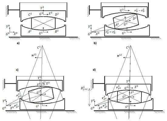
Figure 16.
Stick-Slip Model: (a) initial geometrically compatible configuration at current time step; (b) rotated stick configuration at the end of sticking phase; (c) initial configuration at beginning of Slipping phase; (d) recovered geometrically compatible new configuration.
5.1. Sticking Phase
During the Sticking phase, we assume that the pad (RB2) undergoes a rotation by jamming along its compressed diagonal, which is for . Such behavior is modelled by constraining RB2 to the two concave surfaces and , by means of two pinpoints, placed in the positions occupied by and , respectively, at the end of the previous time step . Thus, in this phase, the non-linear kinematic constraint equations are given by:
in which the fourth and fifth equations impose that the global coordinates of the vertices and assume the same values if written by using either their belonging to RB2, yielding and , or their belonging to RB1 or RB3, respectively, yielding and . These two row vector equations yield:
where the local coordinates and are those at the end of the previous time step . With these equations, the square kinematic constraints Jacobian matrix has all null elements except for the following ones:
where the symbols have the meaning already introduced.
5.2. Slipping Phase
During the Slipping phase, we assume that the pad undergoes a rigid roto-translation, with , the instant center of rotation, moving along the straight line connecting the centers of the two circumferences and , with frictional sliding at the two vertices and , and up to the restoration of geometrical compatibility and closure of the two kinematic pairs. In this phase, the non-linear kinematic constraint equations are given as follows:
where the first and second equations impose that point and , belonging to the RB2, slide along the tangents to the circumferences and in points and , respectively, which are the relative positions of and at the end of the sticking phase. The first two equations are identical to Equations (8) and (11), respectively.
The third equation imposes that , which is the instant center of rotation, translates along the straight line passing through the position of points and , at the end of the sticking phase. This is equivalent to imposing that the projection of the global position vector , along the direction normal to the segment , with versor , is constant and equal to the value assumed at the end of the sticking phase. The fourth equation imposes that also RB3 has to translate along the segment , which is equivalent to imposing that the projection of the global position vector , of the intersection point between and , along the direction is constant and equal to the value assumed at the end of the sticking phase. The third and fourth equations are given by:
where is the unit vector orthogonal to the segment .
The fifth equation is written as:
where is the ordinate of RB3 in the global inertia reference system, necessary to restore the overall geometrical compatibility (Figure 16d), given by:
where and are the distances between the centroid and the most depressed point of the concave surfaces of RB1 and RB3, respectively, and and are the half opening angles defining the convex surfaces of RB2 paired with Rigid Bodies 1 and 3 (Figure 3); the sixth equation imposes that RB3 cannot undergo any rotation.
With these equations, all elements of the kinematic constraints Jacobian matrix are null except for the following ones:
where the meanings of several symbols have already been introduced.
5.3. Numerical Results
For this model, it is not interesting to analyze the interpenetration at the initial time step, since the model itself is based on the assumption that the DFP initially sticks along one diagonal of the pad. Thus, attention will be focused on the time histories for the same two prototypes whose data are listed in Table 1, together with the details of the imposed ground motion. Maximum values of calculated interpenetration are of the same order of magnitude as what was obtained by means of the Compliant Sliding Model, as can be gathered comparing Figure 9 and Figure 17. Of course, due to the fundamental features of this model, being based on a Stick-Slip functioning assumption, the one-diagonal effect is clearly shown also for the DFP1 prototype, even if with relatively less interpenetration with respect to the DFP2 (Figure 17). In fact, with the stick-slip model, the curves representing the interpenetration time history at the endpoints of each diagonal of the pad are superimposed to each other, and reach their peak at different time instants with respect to the endpoints of the other diagonal. In Figure 18, the time histories and for DFP1 are plotted for integration time step , while the results concerning DFP2 for are plotted in Figure 19. Note that the stick-slip behavior yields a secondary oscillation which is clearly visible in the global coordinate time histories and , whose magnitude depends on: (a) the shape of the DFP, (b) the magnitude of the stepwise velocity, and (c) the value of the integration time step . The dependence on the stepwise value of the ground-imposed velocity can be clearly yielded from the plots of and since the maximum amplitude of the sticking-related oscillations is attained at the time instants in which the maximum relative values of are attained (Figure 18 and Figure 19). This is expected indeed since, applying the definition of discrete velocity , we realize that for a constant value of integration time step, the largest values of incremental ground-imposed displacements are attained in correspondence of the relative maximum values of the imposed velocity. Even the dependence on the pad’s shape can be clearly yielded since the maximum values of sticking-related oscillations are relatively larger for DFP2 with respect to DFP1 (Figure 18 and Figure 19). The importance of the instantaneous velocity can also be gathered from Figure 20, in which the configurations (1) at the beginning of the time step, (2) at the end of the sticking phase, and (3) at the end of the slipping phase are plotted for two different instants of the analyzed displacement time history and for DFP1 and DFP2, respectively. In Figure 20a, the three configurations are plotted for DFP1 at the instant , characterized by a relative maximum value of velocity and the RB2 rotation at (1) the beginning of the time step, (2) the end of sticking, and (3) the end of slipping is equal to , , and , respectively. Figure 20b plots the three configurations for DFP2, at instant to which corresponds a relative maximum value of ground velocity and the three values of RB2 rotation result , , and . It is interesting to note that with a properly optimized shape of the pad, even for relatively high values of ground velocity, the sticking-induced rotation is slight, as for DFP1 at . Another thing worth noting is that for the same signs of ground velocity, the working diagonal obtained with the Stick-Slip modelling assumption is always the opposite of the one obtained by applying the Compliant-Sliding. However, if we remove the strong assumption of infinitely rigid bodies, and do take into account their elastic deformability, it seems reasonable to expect that for , the sticking diagonal would be while for , it would be . In fact, if you consider the shear deformation that a rightward ground movement would induce in RB2, it is easy to figure out that the compressed diagonal, which can jam (stick) is the one and vice-versa.
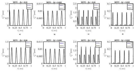
Figure 17.
Time histories of interpenetration, for (a,b) DFP1 and (c,d) DFP2, and for integration time step (a,c) and (b,d).
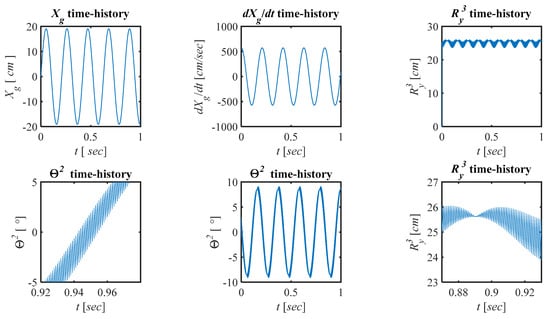
Figure 18.
Numerical results about the DFP1 prototype, for integration time step: global coordinate time histories.
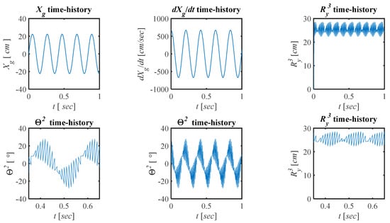
Figure 19.
Numerical results about the DFP2 prototype, for integration time step: global coordinate time histories.
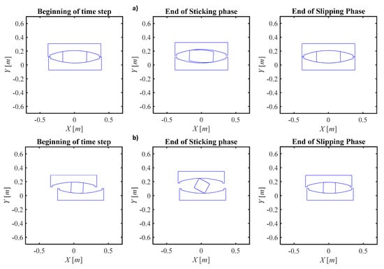
Figure 20.
Two-phase configuration of the analyzed prototypes: (a) DFP1 for integration time step, peak negative value of at , and (b) DFP2 for integration time step, peak negative value of at .
6. Conclusions
After having analyzed in detail the relative movement that the rigid bodies constituting a double friction pendulum (DFP) isolator can undergo during an earthquake in order to fulfill geometrical compatibility, we realized that it cannot be characterized by compliant sliding and a pendulum-like behavior. In fact, the European regulation EN 15129:2009 also renamed these devices as Double Concave Curved Surface Sliders (DCCSS), thus removing the reference to the pendulum.
Moreover, already for the simpler case of a single pendulum, a pendulum-like behavior is numerically possible if the convex component is forced, by means of a torque applied at the extremity of a connecting rod, to rotate around a pinpoint placed right in the center of the coupling concave spherical surface. On the contrary, in the case of friction isolators, an earthquake imposes a kinematic time-history, encompassing displacements, velocities, and accelerations, at the lower plate. For this reason, it is difficult to believe that sliding might take place, already for the single friction pendulum and even more so for the double, in a compliant manner along the coupled spherical surfaces.
Therefore, we have proposed a behavioral model for the DCCSS isolator, capable of fulfilling geometrical compatibility, which envisages a two-step relative movement, named stick-slip. Such modelling strategy assumes that at each time step, the multi-body model undergoes sticking, with temporary loss of geometrical compatibility and change of topology, subsequent slipping concentrated at the endpoints of the compressed diagonal of the pad, and recovery of the initial topology.
Before presenting the multi-body kinematic equations for such devices, developed according to the proposed stick-slip approach, those same equations were also solved for the currently expected behavior, based on compliant sliding, in order to add arguments to the discussion. In this case, taking the pendulum-like behavior for granted, we obtained two strange results, which enforce the idea that the pendulum behavior with compliant sliding is unlikely. Namely, we found that interpenetration of matter is always larger at the endpoints of one of the two diagonals of the pad and, such one-diagonal effect regards, as a function of the sign of the ground-imposed velocity, the diagonal that would result tense, if the elastic deformability of the various elements was taken into consideration. Such results, even more marked for DCCSS isolators characterized by squatter pads, concur to confirm the validity of the initial realization about the real behavior of these devices.
Lastly, the multi-body kinematic equations were applied to model the proposed stick-slip behavior. The obtained results showed that two generalized coordinates, namely the rotation of the pad and the vertical position of the upper sliding plate, undergo a secondary oscillation, whose maximum amplitude is larger for the prototypes with squatter pads, and for larger values of the earthquake-imposed instantaneous velocity.
In this work, for the sake of brevity, the complete dynamics were omitted. However, it will be presented in another work, possibly also including the impact between one another of several rigid bodies and the evaluation of friction-induced heat. Moreover, no attention was paid to the seismological variability of the parameters characterizing the sinusoidal time history adopted to model the earthquake-induced ground motion, since more attention has been paid to the numerical aspects of the modelling strategy. The results in cases of real accelerograms will be presented in a future work.
Author Contributions
Conceptualization, formal analysis, investigation V.B.; seismic engineering supervision G.M.; multi-body methodology N.P.B. All authors have read and agreed to the published version of the manuscript.
Funding
This research received no external funding.
Institutional Review Board Statement
Not applicable.
Informed Consent Statement
Not applicable.
Data Availability Statement
The data presented in this study are available on request from the corresponding author.
Conflicts of Interest
The authors declare no conflict of interest.
Abbreviations
| , | Geometrical quantities defining the pad cross section |
| , | Circumferences characterizing the lower and upper plates concave plates, RB1 and RB3 |
| , | Center of the two concave surfaces of RB1 and RB3, respectively |
| , | Circumferences characterizing the lower and upper convex surfaces of RB2 |
| , | Center of the 2 convex surfaces of RB2, coupled with and , respectively |
| Centroid of the i-th RB | |
| Intersection of the i-th RB circumference and the radius passing through | |
| Intersection of the i-th RB circumference and either one of the straight sides of the pad | |
| , | Radius of the concave surface belonging to RB1 and RB3, respectively |
| , | Radius of the convex surface, of RB2, and coupled with RB1 or RB3, respectively |
| Global abscissa of the local reference system of the i-th RB | |
| Global ordinate of the local reference system of the i-th RB | |
| Initial interpenetration in correspondence of point , along the concave surface of the i-th RB | |
| Time-history of interpenetration in correspondence of point P, along the surface of the i-th RB | |
| i-th RB coordinates transformation matrix | |
| Non-linear kinematic constraints written in vector format | |
| Non-linear kinematic constraints Jacobian Matrix | |
| Vector of the global coordinates of the centroid of the i-th RB | |
| Versor with origin in point P and normal to the i-th RB | |
| Vector of the multi-body system generalized coordinates | |
| Vector of the generalized coordinates of the i-th RB | |
| Global position vector of point P belonging to the i-th Rigid Body | |
| Displacement vector of point P belonging to the i-th RB, with respect to the j-th RB | |
| Local position vector of point P in the reference system of the i-th Rigid Body | |
| Element at the i-th row and j-th column of the Jacobian Matrix | |
| Length of the diagonal of the pad | |
| , | Height of the retaining ring of RB1 and RB3, respectively |
| , | Height of the concave plate, either RB1 or RB3, between most depressed point and opposite flat face |
| Time duration of the ground-imposed time history | |
| Generic time integration instant | |
| , | Thickness of the retaining ring of RB1 and RB3, respectively |
| Local abscissa of point P in the reference system of the j-th RB | |
| Local ordinate of point P in the reference system of the j-th RB | |
| Integration time step | |
| First part (Sticking) of the time step | |
| Second part (slipping) of the time step | |
| Ground-imposed time history | |
| Maximum amplitude of the ground-imposed time-history | |
| , | Half opening angle defining the extension of concave plates RB1 and RB3, respectively |
| , | Opening angle of the convex face of RB2 coupled with either RB1 or RB3 |
| , | Angle between the radius passing through either or , and local axis |
| , | Angle between the radius passing through either or5 , and local axis |
| Counter-clockwise angle formed by the local reference axis with respect to | |
| Angle defining the size of the straight cylinder constituting the pad | |
| Circular frequency of the ground-imposed time history | |
| Vector of the Newton differences |
References
- Zayas, V.A.; Low, S.S.; Mahin, S.A. The FPS Earthquake Resisting System; Report No. 87-01; Earthquake Engineering Research Center: Berkley, CA, USA, 1987. [Google Scholar]
- Mokha, A.; Constantinou, M.C.; Reinhorn, A. Teflon Bearings in Base Isolation, I: Testing. ASCE J. Struct. Eng. 1990, 116, 438–454. [Google Scholar] [CrossRef]
- Constantinou, M.C.; Mokha, A.; Reinhorn, A. Teflon Bearings in Base Isolation, II: Modeling. ASCE J. Struct. Eng. 1990, 116, 455–474. [Google Scholar] [CrossRef]
- Fenz, D.M.; Constantinou, M.C. Behavior of the Double Concave Friction Pendulum Bearing. Earthq. Eng. Struct. Dyn. 2006, 35, 1403–1424. [Google Scholar] [CrossRef]
- Fenz, D.M.; Constantinou, M.C. Spherical Sliding Isolation Bearings with Adaptive Behavior: Experimental Verification. Earthq. Eng. Struct. Dyn. 2008, 37, 185–205. [Google Scholar] [CrossRef]
- Becker, T.C.; Mahin, S.A. Experimental and Analytical Study of the Bi-directional Behavior of the Triple Friction Pendulum Isolator. Earthq. Eng. Struct. Dyn. 2012, 41, 355–373. [Google Scholar] [CrossRef]
- Becker, T.C.; Mahin, S.A. Correct Treatment of Rotation of Sliding Surfaces in Kinematic Model of the Triple Friction Pendulum Bearing. Earthq. Eng. Struct. Dyn. 2012, 42, 311–317. [Google Scholar] [CrossRef]
- Tsai, C.S.; Lin, Y.C.; Su, H.C. Characterization and Modeling of Multiple Friction Pendulum System with Numerous Sliding Interfaces. Earthq. Eng. Struct. Dyn. 2010, 39, 1463–1491. [Google Scholar] [CrossRef]
- Nagarajaiah, S.; Reinhorn, A.M.; Constantinou, M.C. Nonlinear Dynamic Analysis of 3D Base Isolated Structures. ASCE J. Struct. Eng. 1991, 117, 2035–2054. [Google Scholar] [CrossRef]
- Xu, Z.; Du, X.; Xu, C.; Han, R. Numerical analyses of seismic performance of underground and aboveground structures with friction pendulum bearings. Soil Dyn. Earthq. Eng. 2020, 130, 105967. [Google Scholar] [CrossRef]
- Habieb, A.B.; Valente, M.; Milani, G. Effectiveness of different base isolation systems for seismic protection: Numerical insights into an existing masonry bell tower. Soil Dyn. Earthq. Eng. 2019, 125, 105752. [Google Scholar] [CrossRef]
- Almazán, J.L.; De La LLera, J.C.; Inaudi, J.A. Modelling aspects of structures isolated with the friction pendulum system. Earthq. Eng. Struct. Dyn. 1998, 27, 845–867. [Google Scholar] [CrossRef]
- Almazán, J.L.; De La LLera, J.C. Accidental torsion due to overturning in nominally symmetric structures isolated with the FPS. Earthq. Eng. Struct. Dyn. 2003, 32, 919–948. [Google Scholar] [CrossRef]
- Almazán, J.L.; De la Llera, J.C. Analytical model of structures with frictional pendulum isolators. Earthq. Eng. Struct. Dyn. 2011, 31, 305–332. [Google Scholar] [CrossRef]
- Lomiento, G.; Bonessio, N.; Benzoni, G. Friction Model for Sliding Bearings under Seismic Excitation. J. Earthq. Eng. 2013, 17, 1162–1191. [Google Scholar] [CrossRef]
- Sarlis, A.A.; Constantinou, M.A. A model of triple friction pendulum bearing for general geometric and frictional parameters. Earthq. Eng. Struct. Dyn. 2016, 45, 1837–1853. [Google Scholar] [CrossRef]
- De Domenico, D.; Ricciardi, G.; Benzoni, G. Analytical and finite element investigation on the thermo-mechanical coupled response of friction isolators under bidirectional excitation. Soil Dyn. Earthq. Eng. 2018, 106, 131–147. [Google Scholar] [CrossRef]
- Quaglini, V.; Gandelli, E.; Dubini, P. Numerical investigation of curved surface sliders under bidirectional orbits. Ing. Sismica 2019, 36, 118–136. [Google Scholar]
- Ponzo, F.C.; Di Cesare, A.; Leccese, G.; Nigro, D. Standard requirements for the recentering capability of curved surface sliders. Ing. Sismica 2019, 36, 95–106. [Google Scholar]
- Quaglini, V.; Dubini, P.; Poggi, C. Experimental assessment of sliding materials for seismic isolation systems. Bull. Earthq. Eng. 2012, 10, 717–740. [Google Scholar] [CrossRef]
- Ponzo, F.C.; Di Cesare, A.; Leccese, G.; Nigro, D. Shake table testing on restoring capability of double concave friction pendulum seismic isolation systems. Earthq. Eng. Struct. Dyn. 2017, 46, 2337–2353. [Google Scholar] [CrossRef]
- Pavese, A.; Furinghetti, M.; Casarotti, C. Experimental assessment of the cycle response of friction-based isolators under bidirectional motions. Soil Dyn. Earthq. Eng. 2018, 114, 1–11. [Google Scholar] [CrossRef]
- Pigouni, E.A.; Castellano, M.G.; Infanti, S.; Colato, G.P. Full-scale dynamic testing of pendulum isolators (Curved surface sliders). Soil Dyn. Earthq. Eng. 2019, 130. [Google Scholar] [CrossRef]
- Popov, V. Contact Mechanics and Friction-Physical Principles and Applications; Springer: Berlin, Germany, 2010; pp. 175–230. [Google Scholar]
- Belfiore, N.P.; Di Benedetto, A.; Pennestrì, E. Foundations of Mechanics Applied to Machines; Casa Editrice Ambrosiana: Milano, Italy, 2000; pp. 153–194. (In Italian) [Google Scholar]
- Shabana, A.A. Dynamics of Multibody Systems; John Wiley & Sons: New York, NY, USA, 1989; pp. 195–240. [Google Scholar]
- Shabana, A.A. Computational Dynamics; John Wiley & Sons: New York, NY, USA, 2001; pp. 295–378. [Google Scholar]
- Nikravesh, P.E. Planar Multibody Dynamics-Formulation, Programming with MATLAB, and Applications; CRC Press, Taylor & Francis Group: New York, NY, USA, 2018; pp. 355–382. [Google Scholar]
- Bianco, V.; Bernardini, D.; Mollaioli, F.; Monti, G. Modeling of the temperature rises in multiple friction pendulum bearings by means of thermomechanical rheological elements. Arch. Civ. Mech. Eng. 2019, 19, 171–185. [Google Scholar] [CrossRef]
- Bianco, V.; Monti, G.; Belfiore, N.P. New approach to model the mechanical behavior of multiple friction pendulum devices. In Proceedings of the 5th International Conference Integrity-Reliability-Failure, IRF2016, Porto, Portugal, 24–28 July 2016. [Google Scholar]
- Bianco, V.; Monti, G.; Belfiore, N.P. Complete analytical thermo-mechanical model of double friction pendulum devices. In Proceedings of the COMPDYN 2017, 6th ECCOMAS Thematic Conference on Computational methods in Structural Dynamics and Earthquake Engineering, Rhodes Island, Greece, 15–17 June 2017. [Google Scholar]
- Bianco, V.; Monti, G.; Belfiore, N.P. Mechanical Modelling of Friction Pendulum Isolation Devices. In Proceedings of Italian Concrete Days 2016, Lecture Notes in Civil Engineering; Di Prisco, M., e Menegotto, M., Eds.; Springer: Cham, Switzerland, 2018; pp. 133–146. [Google Scholar]
- Bianco, V.; Monti, G.; Belfiore, N.P. Fine-tuning of modelling strategy to simulate thermo-mechanical behavior of double friction pendulum seismic isolators. NED Univ. J. Res. 2020, 3. [Google Scholar] [CrossRef]
- Mariti, L.; Belfiore, N.P.; Pennestrì, E.; Valentini, P.P. Comparison of Solution Strategies for Multibody Dynamics Equations. Int. J. Numer. Methods Eng. 2011, 88, 637–656. [Google Scholar] [CrossRef]
- Italian Ministry of Infrastructures and Transport. Italian Technical Regulations, Technical Standards for Construction (NTC2018); Italian Ministry of Infrastructures and Transport: Rome, Italy, 2018. [Google Scholar]
- European Committee for Standardization (CEN). Eurocode 8. Design of Structures for Earthquake Resistance-Part 1: General Rules, Seismic Actions and Rules for Buildings (UNI EN 1998-1); European Committee for Standardization (CEN): Brussels, Belgium, 2004. [Google Scholar]
- CEN. European Standard EN 15129:2009:E Anti-Seismic Devices; CEN: Brussels, Belgium, 2009. [Google Scholar]


Publisher’s Note: MDPI stays neutral with regard to jurisdictional claims in published maps and institutional affiliations. |
© 2021 by the authors. Licensee MDPI, Basel, Switzerland. This article is an open access article distributed under the terms and conditions of the Creative Commons Attribution (CC BY) license (http://creativecommons.org/licenses/by/4.0/).