Automated Generation of an Energy Simulation Model for an Existing Building from UAV Imagery

Abstract

An approach to automatically generate a dynamic energy simulation model in Modelica for a single existing building is presented. It aims at collecting data about the status quo in the preparation of energy retrofits with low effort and costs. The proposed method starts from a polygon model of the outer building envelope obtained from photogrammetrically generated point clouds. The open-source tools TEASER and AixLib are used for data enrichment and model generation. A case study was conducted on a single-family house. The resulting model can accurately reproduce the internal air temperatures during synthetical heating up and cooling down. Modelled and measured whole building heat transfer coefficients (HTC) agree within a 12% range. A sensitivity analysis emphasises the importance of accurate window characterisations and justifies the use of a very simplified interior geometry. Uncertainties arising from the use of archetype U-values are estimated by comparing different typologies, with best- and worst-case estimates showing differences in pre-retrofit heat demand of about ±20% to the average; however, as the assumptions made are permitted by some national standards, the method is already close to practical applicability and opens up a path to quickly estimate possible financial and energy savings after refurbishment.

1. Introduction

The buildings sector is directly or indirectly responsible for 18.4% of total anthropogenic greenhouse gas emissions [1]. Reducing this impact is one of the key issues for mitigating global warming. For a pathway that aims at limiting global warming to an average temperature increase of 1.5 °C, existing buildings should be renovated at a rate of 5% per year by 2020 [2]. This benchmark number is far from being reached: In the EU, the weighted annual renovation rate is at about 1% [3]. Nevertheless, countries have implemented different policies. These include minimum requirements for energy retrofits of existing buildings and rules for their execution. As the first step of renovation measures, the laws usually demand an analysis of the current state, e.g., by energy consultants. They evaluate the status quo energy performance according to national or international standards and give recommendations for suitable retrofit measures. For the post-retrofit state, requirements regarding overall energy demand, thermal transmittance (U-values) of certain building parts, or whole building heat transfer coefficients (HTC) apply [4].

The associated calculations require knowledge about certain boundary conditions as well as about the geometry and the fabric of the building. Most parameters can be individually assessed: For example, blower-door tests can determine the airtightness [5] and heat flow sensors can be used to measure the U-value of building parts [6]. Besides more or less advanced measurement devices, available plans of the building are an important source for geometric dimensions [7]. To keep the measurement effort for individual building analysis reasonably low, standards and laws give room for assumptions and provide default values. For example, air exchange rates for certain situations [8] and heat conductivities of certain building materials [9] can be used. In Germany, the German Meteorological Service (DWD) offers representative weather data as test reference years [10]. Furthermore, the legislation allows to use “simplified measurements” and “empirical values for building parts and system components of comparable age classes” if no better knowledge about the building is available [11]. A similar approach exists as Reduced Standard Assessment Procedure (RdSAP) in the United Kingdom [12]. Although such simplifications are important to keep the effort small, they cause inaccuracies that are one reason for the so-called “performance gap” between predicted demand and actual energy use [13].

One possibility for mitigating these inaccuracies is the whole building’s qualification by measurement of its HTC. Several methods are able to determine this metric, for example the evidently reliable co-heating test [14] or the QUB method [15]. They have the advantages of directly measuring the actual energy performance and not requiring the geometry or similar preliminary knowledge of the building. Their drawbacks are that they cannot be the only source of information for individual envelope component refurbishment, that solar gains and air exchange need to be accounted for with additional measurements and modelling effort, and the need for an unoccupied building. If such dedicated measurement campaigns should be avoided, some available approaches are the energy signature method [16], grey-box regression [17], or modelling based on data from smart meters or building automation systems [18,19]. Similar approaches can also be used to calibrate existing models [20]. The further spread of smart meters and smart home devices may enable the wider application of these tools, which is currently limited by the need for a comparatively long time series of data that can only be meter-read or measured using dedicated equipment, meaning an amount of work that is unreasonably high for small building retrofit preparations. A more technologically complex approach to reduce the data acquisition effort is the automation of the measurement and the “white-box” [21] modelling process. Regarding the geometry, terrestrial laser scans (TLS) or images obtained from unmanned aerial vehicles (UAVs, also known as drones) can be applied to create accurate point cloud or mesh representations of the building envelope [22,23,24]. Commercial software allows to manually extract surfaces and to create models for building information modelling (BIM) from the point clouds. They may also include interior surface information from original [24] or TLS-reconstructed [25] floor plans. Regarding thermal parameters, data from infrared thermography (IRT) are useful for qualitative inspections, but faces limited applicability in quantitative studies due to a lack of accuracy [26,27]. As a consequence, material information or thermal parameters are sourced from previously known information or the aforementioned measurement methods. After adding these data to BIM, interfaces to building energy models (BEM) enable energy simulations. The use of established software makes this approach pragmatic, but individual modelling effort is high [28]. To achieve a suitable cost–benefit ratio that is necessary for increasing renovation rates and to compensate the limited availability of skilled labour, further automation of the whole process is highly desirable.

In urban building energy modelling (UBEM), the need for reconstruction and modelling of large datasets has led to the development of largely automated approaches. Simplified geometries with semantic annotations are reconstructed from remotely sensed point clouds [29,30]. Using these or open data as a source, several tools are able to estimate building energy demands on a large scale (see e.g., the reviews on the field by Reinhart and Cerezo Davila [31] or Sola et al. [32]). During that process, models are often enriched with common “archetype” building properties. For example, the open-source tool TEASER [33] contains data from the TABULA project [34] to assign common envelope component layers to residential buildings depending on their age and size class and creates a dynamic energy simulation model applying the Modelica library AixLib [35]. For these applications on urban scale, the modelling accuracy of individual buildings is reduced in favour of less computational effort, maintaining adequate accuracy on an aggregated level. The latter was confirmed for the combination of TEASER and AixLib by Remmen et al. [33] and Lauster and Müller [36]. To increase individual building accuracy, promising calibration approaches exist [37]; however, they require substantial time series data to be collected in advance, which is again unsuitably laborious for small retrofit projects.

The approach presented in this paper applies UBEM data enrichment and simulation tools to a single building, with the goal of providing information for individual retrofits. It uses accurate geometry information that can be obtained using UAVs, shows how the whole process can be highly automated, and avoids some simplification steps in the generation of the energy simulation model that are commonly used in automated model generation at district and city scale. In this way, a model for dynamic energy simulation is generated with minimal user interaction. The paper includes a case study as a first step towards validation.

The article is structured as follows: In Section 2, the approach is presented, consisting of the creation of a polygonal 3D model from photogrammetry, data enrichment from available knowledge and typologies, and the generation of a simulation model using an interface between Python and Modelica. The case study building to which it was applied is introduced as well. Section 3 describes the results of modelling and simulation. Their relationship to the actual conditions of the case study building concerning the dynamic behaviour during a measurement campaign and to its theoretical heat demand and HTC is discussed. In the final section, conclusions are drawn on the applicability of the approach in practice and how it could benefit from additional research in remote sensing technology.

2. Methods

The goal of this study is to demonstrate how largely automatable processes starting from UAV-based remote sensing can be used to generate a building energy simulation model. The steps of the approach are depicted in Figure 1. For the case study of a single-family house, the geometry is modelled based on close-range aerial imagery. After the model is augmented by additional simple pieces of information about the house (e.g., year of construction and basement height) acquired from owners or inhabitants, it is enriched with energetically relevant properties and processed to a Modelica simulation model using the open-source tools TEASER [33] and AixLib [35]. Several variations of the model are created to determine the sensitivity of the simulation results to differences in the building parameters. With the simulation models, the dynamic behaviour during a measurement campaign is computed and the annual heat demand as well as the HTC of the building are derived.

In the following, the case study building is described and the steps are explained, illustrated by exemplary data from the case study.

2.1. Case Study Building

An unoccupied single-family house located in a rural neighbourhood and constructed around 1965 was used for the case study. Above its full cellar, two heated stories cover a total floor area of about 117 m². An unheated attic is located beneath the roof. The windows were replaced in the mid-1990s.

During a measurement campaign in February 2019, the building was heated for several days using distributed electrical heaters and fans, was kept at an approximately constant mean interior temperature of above 30 °C for seven days, and was afterwards exposed to free cooling. Meanwhile, interior temperatures, heating loads, and exterior conditions were monitored.

From construction plans, on-site inspections (including drillings), and material tests, information designed to serve as reference values for the presented approach was collected.

The complimentary dataset provided for this paper contains floor plans of the building, recordings from the measurement campaign, and additional data that are mentioned further on in this paper [38].

2.2. Data Collection

Portraying the geometry is the first step of white-box building modelling. In this case, the source for the geometry is a CityGML file containing above-ground outside surfaces of walls, roofs and windows. The file is available in the dataset [38]. It was created from a point cloud of the building’s envelope that has been obtained photogrammetrically from high-resolution RGB images. The images had been captured with a standard digital single-lens reflex camera mounted on a UAV. With the point cloud (visualised in Figure 2) as input, the method of Frommholz et al. [29] delivered a textured 3D polygonal model of the building envelope. Windows were recognised on the textures using a colour-based approach [39]. CityGML was chosen as the data exchange format due to its comprehensible structure combining semantic and positional data and because it was designed to be created from measurements, which makes it more suitable for surface-based modelling tasks than the BIM formats usually created during a building design phase [40].

After importing the geometry from the CityGML file into a custom building model programmed in Python, additional information is introduced. First, the window polygons are exploited to separate the buildings into storeys (see Figure 3): Windows are classified as French or other windows and those with overlapping vertical position are collected, assuming they belong to the same storey. The vertical position of floors of storeys with French windows is directly below their lower edge. For storeys without French windows, the common window cill height of 0.85 m according to the German technical standard DIN 5034-4 [41] is assumed as the distance between the floor and the median of the lower window edges. The median has the advantage of cancelling out possible staircase windows. The ceiling thicknesses are assumed as 0.3 m, the height of the uppermost storey is derived from the average height of other storeys (if necessary, which was not the case here due to the attic windows), and the floor-to-ceiling height of the basement is obtained from owners or inhabitants (here: 2.07 m). Thus, all ceiling positions can be derived and volumetric room objects for each storey are created in the Python model. The exterior shape of the resulting model is visualised in Figure 2.

Additional simple information from owners or inhabitants enrich the model by defining storeys as heated or unheated, by specifying the year of construction of the building as a whole and of the individual windows, and by enabling the choice of default airtightness values for unconditioned spaces according to Table 7 in ISO 13789 [8]. In this case, the attic and the basement are unheated and their air exchange rates are assumed as 10 h^$-1$ and 1 h^$-1$, respectively.

2.3. Data Enrichment and Interface to Simulation

For performing building energy simulations, the model requires thermal parameters of the building parts and use conditions of the zones as well as an interface to a simulation tool. Both data enrichment and interface are offered by the open-source Python module TEASER [33]; therefore, the information stored in the custom Python model is transferred to a TEASER model of the building. In that process, the data are enriched by default use conditions, area of internal walls, ceilings and floors, and building part materials from the German TABULA typology [34].

TEASER was designed for urban energy modelling of archetypal buildings. The application presented in this study demanded to improve its applicability to single buildings. For this purpose, several parts of the code were modified. First, the archetype building creation process was expanded by additional parametrisation options. In the adjusted workflow, component attributes such as areas, orientations, and layer structures are introduced. Second, an attribution of a neighboured zone to inner walls was made possible in order to enable the modelling of zone borders. Previously, the different zones within a building were modelled without interaction between them. Third, the generation of the simulation model from the stored data was modified. TEASER offers an interface to the “ReducedOrder” model (ROM) of the likewise open-source Modelica library AixLib [35]. The export process includes lumping multiple heat-transferring components to a single resistance-capacitance (RC) element according to the guideline VDI 6007 Part 1 [42]. Windows are modelled separately. For urban simulations, a two-element model with one element lumping all roofs, outer walls, and ground floors and a second one for internal structures offers a reasonable accuracy at low simulation times [43]. For single buildings, some simplifications can be avoided in favour of a higher accuracy. To do so, the respective parts of the AixLib ROM were modified along with the TEASER algorithms. First, the previously largely neglected differences in dynamic thermal behaviour between building parts with different exposition to radiation are accounted for. This is achieved by reducing the lumping to one element per component type and exterior orientation. Additional elements cover the borders between heated and unheated spaces. The resulting configuration is visualised in Figure 4. Furthermore, the assumption that all outside surfaces exchange longwave radiation only with the sky tends to cause an underestimation of exterior surface temperatures. It is removed by introducing a possibility to source weather data from DWD test reference years (TRY), which include terrestrial longwave radiation and by modifying the implementation of calculating the heat exchange with the exterior. In the calculations according to VDI 6007 Part 1 [42], the heat flux q from the exterior space to an exterior surface with surface temperature $T_{\mathrm{se}}$ is computed as

$$q=h_{\mathrm{comb},\mathrm{se}}·\left(T_{\mathrm{eq},\mathrm{se}}-T_{\mathrm{se}}\right)$$

(1)

by merging radiant and convective heat transfer coefficients of the surface to a combined coefficient $h_{\mathrm{comb},\mathrm{se}}$ and using the equivalent outdoor temperature

$$T_{\mathrm{eq},\mathrm{se}}=T_{\mathrm{amb}}+\Delta T_{\mathrm{eq},\mathrm{sw},\mathrm{se}}+\Delta T_{\mathrm{eq},\mathrm{lw},\mathrm{se}}$$

(2)

that is based on the (dry-bulb) ambient temperature $T_{\mathrm{amb}}$ and includes a contribution of shortwave (solar) radiation $\Delta T_{\mathrm{eq},\mathrm{sw},\mathrm{se}}$ and of longwave radiation $\Delta T_{\mathrm{eq},\mathrm{lw},\mathrm{se}}$. The previous implementation in AixLib computes the latter from the difference between air temperature and black sky temperature $T_{\mathrm{sky}}$ (derived from atmospheric longwave radiation) as

$$\Delta T_{\mathrm{eq},\mathrm{lw},\mathrm{se}}=\left(T_{\mathrm{sky}}-T_{\mathrm{amb}}\right)·\frac{h_{\mathrm{rad},\mathrm{se}}}{h_{\mathrm{comb},\mathrm{se}}},$$

(3)

where $h_{\mathrm{rad},\mathrm{se}}$ is the radiant heat transfer coefficient for the surface. The newly implemented algorithm follows the guideline except for the influences of horizon elevation and a radiation-dependent radiant heat transfer coefficient, leading to

$$\Delta T_{\mathrm{eq},\mathrm{lw},\mathrm{se}}=\left(\sqrt[4]{\frac{-E_{\mathrm{ter},\mathrm{lw}}}{0.93·\sigma }}·\left(1-F_{\mathrm{se},\mathrm{sky}}\right)+\sqrt[4]{\frac{E_{\mathrm{atm},\mathrm{lw}}}{0.93·\sigma }}·F_{\mathrm{se},\mathrm{sky}}-T_{\mathrm{amb}}\right)·\frac{{\epsilon }_{\mathrm{se}}·h_{\mathrm{se},\mathrm{rad}}}{h_{\mathrm{se},\mathrm{comb}}·0.93},$$

(4)

where $E_{\mathrm{ter},\mathrm{lw}}$ is the terrestrial longwave radiation (which is defined downward in the TRYs and therefore always negative), $E_{\mathrm{atm},\mathrm{lw}}$ is the atmospheric longwave radiation, ${\epsilon }_{\mathrm{se}}$ is the longwave emissivity, and

$$F_{\mathrm{se},\mathrm{sky}}=\frac{1+cos{\gamma }_{\mathrm{tilt},\mathrm{se}}}{2}$$

(5)

is the sky view factor of the surface, calculated from its tilt angle ${\gamma }_{\mathrm{tilt},\mathrm{se}}$.

The resulting workflow makes it possible to generate a dynamic energy simulation model in Modelica from the measured polygonal 3D geometry of an existing building, with energetically relevant parameters mostly originating from the typology. The model can be applied to calculate the building’s annual heat demand and to simulate its thermal behaviour under predefined boundary conditions.

2.4. Model Variations and Sensitivity Analysis

In order to determine the sensitivity of the simulation results to differences in the building parameters, simulation models of the case study building were created in six different variations. Variations 1 to 4 represent an increasing amount of information acquired on site that is introduced into the model. Variation 5 and 6 are used for analysing the confidence region of the simulation results of variation 3, containing best-case and worst-case archetype U-values. The key parameters are listed in

Table 1. Building part heat transfer coefficients (U-values), window solar heat gain coefficients (SHGC) and interior surface areas of different variations of the simulation model for the case study building. Window U-values are always 1.9 Wm⁻² K⁻¹. Brackets indicate U-values of envelope components of unheated spaces from which inappropriate insulation layers were removed.

Var. No.	U-Value Source	(Mean) U-Values [Wm−2 K−1]				SHGC	$A_{\mathrm{int}}$
		Roofs	Ext. Walls	Attic Floor	Basem. Ceil.
1	TABULA	0.9 (3.2)	1.2	0.8	1.1	0.6	376
2	TABULA	0.9 (3.2)	1.2	0.8	1.1	0.36	376
3	TABULA	0.9 (3.2)	1.2	0.8	1.1	0.36	265
4	Best guess	0.4 (6.7)	1.3 (1.8)	0.5	1.1	0.36	265
5	Best case	0.7 (3.2)	0.9 (1.7)	0.7	0.8	0.36	265
6	Worst case	1.8 (3.2)	1.7	1.3	1.3	0.36	265

. The dataset [38] contains a table of all Modelica model parameters and TEASER-compatible JSON files for each variation.

Regarding the U-values, variations 1 to 3 use the TABULA values [34] as implemented in TEASER. Variation 4 contains the best knowledge from building plans and on-site investigations about the walls (exterior and interior) and the roof of the building. As the actual compositions of the building parts in contact to soil and of the basement ceiling are unknown, it falls back to TABULA values there. Variations 5 and 6 reflect the best- and worst-case, respectively, when considering the building typology for the German state of North Rhine-Westphalia [45] where the case study building is located. They are a remedy for the unavailability of uncertainty information on TABULA’s archetype building components and can be understood as the boundary of the confidence region for the thermal parameters of the building. As the time of window installation was known to be more recent than the state typology, their U-values were not varied.

The variations also differ in the solar heat gain coefficient (SHGC) of the windows and in interior component surface areas to assess the model sensitivity for these parameters. Variations 2 to 6 use a reduced SHGC that accounts for the fact that the window recognition process yields window areas including frames, but the typology SHGC value refers to the glazed area. The implied glazing-to-frame area ratio of 1.5 results from observations on site. Variations 1 and 2 use an estimation for the interior component area (including walls, floors, and ceilings) that assumes rooms with a standard size of 6 m × 3 m. In the original implementation of TEASER, the floor area is separated into rooms and one wall per room is considered an exterior wall [36]. Although the estimation approach applies a modified formula that also considers the actual footprint and therefore does not overestimate thermal mass as much as the original one, the values are still higher than the reference values (see Section 2.1) of the building implemented in variations 3 to 6.

In all cases, the model consists of three thermal zones: attic, basement, and one heated zone that covers all the living area in the ground and first floor. Two small unheated spaces between the roof and a part of the first floor are modelled as part of the heated zone as they are not visible from the outside.

3. Simulation Results and Discussion

On the simulation models generated from the variations described in Section 2.4, three different types of computations were performed. First, the measurement campaign was simulated using the recorded exterior conditions and heat loads. Second, the annual heat demands for the existing building and a refurbishment scenario of each variation were determined using the local test reference year. Third, the HTC of the whole building was calculated, simulating a steady state situation. In this section, the results are presented and discussed.

3.1. Simulation of the Measurement Campaign

To test the ability of the model to reproduce the dynamic thermal behaviour of the building, the simulated interior temperatures of the model variations 1 to 4 under the conditions recorded during the measurement campaign (described in Section 2.1) are compared to the measured ones. Figure 5 shows measured and simulated values of the mean air temperature of the building’s heated zone over the course of the campaign. The comparison of the five graphs leads to several observations:

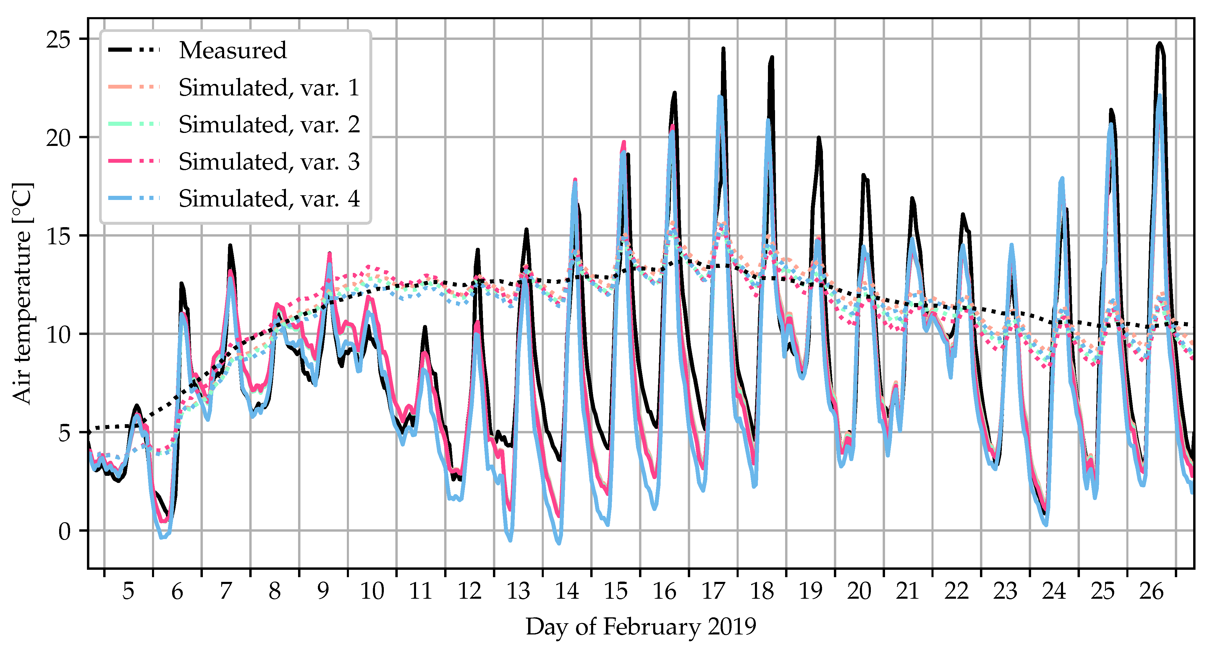
• All in all, the simulated temperatures, in particular of variation 4, match the measured temperatures well, especially when considering that the zone is actually divided into six rooms of which one (the kitchen, located in the ground floor) heated up much more quickly than the others and kept a temperature of about 37 °C from February 9 until the start of the cooldown due to the placement of the largest heater. Furthermore, the influence of the fans (intended to homogenise air temperatures) on convection was not modelled;
• The temperatures on February 13 and afterwards show that variation 1 overestimates daily temperature oscillation. With window SHGC and therefore solar gains reduced, the other model variations are more consistent with the measured temperatures during the period of approximately constant temperature between February 13 and 16;
• When comparing variations 2 and 3, the reduced interior thermal mass in variation 3 makes the simulated temperatures fit better to the measured values during the cooldown phase, but overshoot during heating up;
• Variation 4, which represents the best knowledge of the building and should therefore create the best temperature fit, reproduces the temperatures better than the other variations until the beginning of cooling down and is still reasonably accurate afterwards. The slight mismatch in the speed of heating up and cooling down cannot be caused by deviations of the thermal transmittance of the building envelope as temperatures fit well between February 10 and 16. A possible explanation is that the simplified resistance-capacitance representation of the exterior walls in Modelica cannot exactly model the dynamic behaviour of the actual walls. They are mostly composed of lightweight concrete with low heat capacity on the inside and bricks with high heat capacity on the outside and therefore will store heat further outside than their model representation and react faster to changes in the heat flow from the building interior;
• The agreement between simulated and measured temperatures is even better than the one of a simulation model based on German archetypes to a detailed simulation of a similar Belgian house in the original publication on TEASER [33]; therefore, the good agreement points towards the validity of the overall approach, at least for this specific age and size class.

In Figure 6, the mean air temperatures of the unheated zones (basement and attic) are visualised. The difference between measured and simulated temperatures varies and reaches up to 5 K for a few points in time. Given the intense dynamics, this can be considered a satisfactory agreement between simulated and measured temperatures; however, it stands out that modelled basement temperatures of February 11 and afterwards oscillate more than the measured temperatures. Most likely, the reason is an overestimation of the air exchange rate. Other possible explanations are an overestimation of the impact of solar gains on the heat flow from the ground floor to the basement or an underestimation of the thermal masses in the basement.

3.2. Determination of the Heat Demand

The annual heat demands for all six model variations were calculated running simulations for the complete DWD test reference year. Additionally, a retrofit scenario for each of them was created using the additional insulation layers applied by the TABULA standard retrofit scenario [34] as implemented in TEASER.

The results without retrofit in Figure 7 show that the increased SHGC of variation 1 leads to a considerable reduction in heat demand compared to variation 2. This illustrates the importance of not just detecting the window openings, but also the frame portion of the existing windows when generating a building model automatically from remote sensing data.

In contrast to that, the difference in internal thermal mass has almost no impact on the heat demand. It must be noted that the simulations were made without any set-point reduction in the heating during the night (which is the default setting in TEASER). Introducing set-point reduction may result in higher impacts of the internal thermal mass.

On the one hand, the small difference between variations 3 and 4 shows that the case study building is a good representative of its TABULA type. On the other hand, the high difference between the heat demands of variations 5 and 6 may give a feeling for the width of the distribution of energy performances of buildings with similar age and construction type and illustrate that the randomly chosen case study building could as well have been more or much less energy-efficient. Even though the demands in the retrofit scenarios do not differ considerably between best and worst case, owners would choose their retrofit options based on savings compared to the status quo. This emphasises the high importance for the difference between the heat demands in the existing state and a potential retrofit scenario. At this point, it becomes clear that the overall reliability of the approach would benefit from an increased accuracy in the measurement of U-values by complimentary remote sensing techniques; however, measurements through quantitative infrared thermography [26] currently must be considered more uncertain than typology values and other standard procedures [6,46] are too laborious for the goal of this approach.

3.3. Determination of the Heat Transfer Coefficient (HTC)

Figure 8 shows calculated and measured HTC values for the case study building. The measured one was derived from a period during the measurement campaign with approximately constant ambient and interior air temperatures. For the steady state simulation results, the soil temperature was assumed equal to the ambient temperature, which reflects the situation during the measurement. Nevertheless, values are generally below those calculated according to ISO 13789 [8]. The ISO standard does not account for solar gains and interior thermal masses, which results in equal values for the model variations 1 to 3. The AixLib simulation model includes radiative heat transfer between interior surfaces of envelope components and interior component surfaces, leading to a slightly lower HTC in variation 3 where the latter is smaller.

All in all, HTC values simulated through the realistic model variations (1 to 4) are within a 12% range below the measured value. As the circumstances (simple geometry of the building, relatively accurate U-values in the model) are beneficial, this range cannot be taken as the general uncertainty of the method. For example, increased convection caused by the fans leads to an increase in the measured HTC. For variation 3, increasing the internal convection coefficients of the heated zones by 4 Wm⁻² K⁻¹ (which is equivalent to an increase in the wind speed of 1 ms⁻¹ when concerning ISO 6946 [47]) leads to a simulated HTC value of 382.5 WK⁻¹. Furthermore, the best-/worst-case model variations (5 and 6) lead to a difference to the measured value of $-24$% and $+20$%, respectively. As a consequence, accurate U-values measured by infrared thermography or other techniques again would be a valuable improvement; however, the fact that the HTC does not account for solar gains, air infiltration, and interior thermal masses makes it measurable through the presented method with smaller uncertainty than the heat demand. This is also illustrated by the low or non-existing differences between variations 1 to 3.

4. Conclusions and Outlook

The article has presented an approach to automatically generate a Modelica energy simulation model for an existing building from a point cloud derived from remote sensing using a Python building model and the open-source tools TEASER and AixLib. TEASER and the reduced-order model in AixLib were modified for the use case of modelling single residential buildings based on measured data enriched with typology parameters. Thus, the applicability of their combination for simulating such buildings was demonstrated. For a single-family house as a case study building, the model can accurately reproduce the internal temperatures during a 21-day measurement campaign in which the building was heated up and freely cooled afterwards. Using test reference years as weather data, the annual heat demand for the existing state and for retrofit scenarios can be calculated. As a consequence, the approach has the potential to quickly, automatically, and therefore inexpensively calculate pre- and post-retrofit heat demand estimates and, hence, compare possible savings of potential refurbishment scenarios.

Whole building heat transfer coefficients calculated through the model match values calculated according to ISO 13789 (2017) well and show deviations between $-8$% and $-12$% compared to the measured value.

For the accuracy of the simulation results, the study emphasises the importance of solar gains, while interior thermal masses appear to be less vital. To increase the fidelity of the former, the window recognition process should be improved. Regarding the latter, the presented method can be considered to model it well enough. Due to missing data, the uncertainty of the U-values from the typology cannot be determined, but best- and worst-case estimates showing differences of about ±20% to the average values give a feeling for the magnitude of the confidence region; however, using characteristic U-values is allowed by German legislation; therefore, the presented approach is already close to practical applicability and can supply energy consultants with a useful building energy simulation model as soon as interfaces to the commonly used software packages are created.

The generated model would benefit from measured U-values nevertheless; therefore, one of the next steps is to improve the accuracy of quantitative infrared thermography and include it into the method. It may also be applied using UAVs and could be combined with wall structure analysis by microwave radar [48]. Further possible improvements include the use of faster measurement approaches for airtightness [49], an interface to common BIM software, and the addition of a tool for the economic evaluation of potential retrofit scenarios.

References

1. IPCC. Climate Change 2014: Synthesis Report. Contribution of Working Groups I, II and III to the Fifth Assessment Report of the Intergovernmental Panel on Climate Change; IPCC: Geneva, Switzerland, 2015. [Google Scholar]
2. Kuramochi, T.; Höhne, N.; Schaeffer, M.; Cantzler, J.; Hare, B.; Deng, Y.; Sterl, S.; Hagemann, M.; Rocha, M.; Yanguas-Parra, P.A.; et al. Ten key short-term sectoral benchmarks to limit warming to 1.5 °C. Clim. Policy 2018, 18, 287–305. [Google Scholar] [CrossRef]
3. European Commission. A Renovation Wave for Europe—Greening our Buildings, Creating Jobs, Improving Lives: COM/2020/662 Final; Communication from the Commission to the European Parliament, the Council, the European Economic and Social Committee and the Committee of the Regions: Brussels, Belgium, 2020. [Google Scholar]
4. Rodríguez-Soria, B.; Domínguez-Hernández, J.; Pérez-Bella, J.M.; Del Coz-Díaz, J.J. Review of international regulations governing the thermal insulation requirements of residential buildings and the harmonization of envelope energy loss. Renew. Sustain. Energy Rev. 2014, 34, 78–90. [Google Scholar] [CrossRef]
5. ISO 9972:2014-08. Thermal Performance of Buildings: Determination of Air Permeability of Buildings: Fan Pressurization Method; International Organization for Standardization: Geneva, Switzerland, 2014. [Google Scholar]
6. ISO 9869-1:2014-08. Thermal Insulation: Building Elements: In-Situ Measurement of Thermal Resistance and Thermal Capacitance: Heat Flow Meter Method; International Organization for Standardization: Geneva, Switzerland, 2014. [Google Scholar]
7. Balkowski, M.; Jagnow, K. Datenaufnahme Gebäudehülle. In Leitfaden Energieausweis. Teil 1 – Energiebedarfsausweis: Datenaufnahme Wohngebäude; Deutsche Energie-Agentur (Dena), Ed.; Dena: Berlin, Germany, 2015; pp. 23–46. [Google Scholar]
8. ISO 13789:2017-06. Thermal Performance of Buildings: Transmission and Ventilation Heat Transfer Coefficients: Calculation Method; International Organization for Standardization: Geneva, Switzerland, 2017. [Google Scholar]
9. Anderson, B.; Doran, S.; Mina, K.; Pettit, G. Thermal properties of building structures. In Environmental Design; CIBSE, Ed.; CIBSE: London, UK, 2006. [Google Scholar]
10. Deutscher Wetterdienst; Bundesamt für Bauwesen und Raumordnung. Ortsgenaue Testreferenzjahre von Deutschland für Mittlere, Extreme und Zukünftige Witterungsverhältnisse: Handbuch. Available online: https://www.bbsr.bund.de/BBSR/DE/forschung/programme/zb/Auftragsforschung/5EnergieKlimaBauen/2013/testreferenzjahre/try-handbuch.pdf (accessed on 9 November 2020).
11. Bundestag. Gebäudeenergiegesetz. BGBL I (Bundesgesetzblatt Teil I) 2020, 37, 1728. [Google Scholar]
12. Kelly, S.; Crawford-Brown, D.; Pollitt, M.G. Building performance evaluation and certification in the UK: Is SAP fit for purpose? Renew. Sustain. Energy Rev. 2012, 16, 6861–6878. [Google Scholar] [CrossRef]
13. van den Brom, P.; Meijer, A.; Visscher, H. Performance gaps in energy consumption: Household groups and building characteristics. Build. Res. Inf. 2018, 46, 54–70. [Google Scholar] [CrossRef] [Green Version]
14. Jack, R.; Loveday, D.; Allinson, D.; Lomas, K. First evidence for the reliability of building co-heating tests. Build. Res. Inf. 2018, 46, 383–401. [Google Scholar] [CrossRef] [Green Version]
15. Alzetto, F.; Pandraud, G.; Fitton, R.; Heusler, I.; Sinnesbichler, H. QUB: A fast dynamic method for in-situ measurement of the whole building heat loss. Energy Build. 2018, 174, 124–133. [Google Scholar] [CrossRef]
16. Belussi, L.; Danza, L.; Meroni, I.; Salamone, F. Energy performance assessment with empirical methods: Application of energy signature. Opto-Electron. Rev. 2015, 23, 83–87. [Google Scholar] [CrossRef] [Green Version]
17. Hollick, F.P.; Gori, V.; Elwell, C.A. Thermal performance of occupied homes: A dynamic grey-box method accounting for solar gains. Energy Build. 2020, 208, 109669. [Google Scholar] [CrossRef]
18. Crawley, J.; McKenna, E.; Gori, V.; Oreszczyn, T. Creating Domestic Building Thermal Performance Ratings Using Smart Meter Data. Build. Cities 2020, 1, 1–13. [Google Scholar] [CrossRef]
19. Erkoreka, A.; Garcia, E.; Martin, K.; Teres-Zubiaga, J.; Del Portillo, L. In-use office building energy characterization through basic monitoring and modelling. Energy Build. 2016, 119, 256–266. [Google Scholar] [CrossRef]
20. Coakley, D.; Raftery, P.; Keane, M. A review of methods to match building energy simulation models to measured data. Renew. Sustain. Energy Rev. 2014, 37, 123–141. [Google Scholar] [CrossRef] [Green Version]
21. Foucquier, A.; Robert, S.; Suard, F.; Stéphan, L.; Jay, A. State of the art in building modelling and energy performances prediction: A review. Renew. Sustain. Energy Rev. 2013, 23, 272–288. [Google Scholar] [CrossRef] [Green Version]
22. Eschmann, C.; Kuo, C.M.; Kuo, C.H.; Boller, C. High-Resolution Multisensor Infrastructure Inspection with Unmanned Aircraft Systems. ISPRS-Int. Arch. Photogramm. Remote Sens. Spat. Inf. Sci. 2013, XL-1/W2, 125–129. [Google Scholar] [CrossRef] [Green Version]
23. Küng, O.; Strecha, C.; Fua, P.; Gurdan, D.; Achtelik, M.; Doth, K.M.; Stumpf, J. Simplified Building Models Extraction from Ultra-Light UAV Imagery. ISPRS-Int. Arch. Photogramm. Remote Sens. Spat. Inf. Sci. 2011, XXXVIII-1/C22, 217–222. [Google Scholar] [CrossRef] [Green Version]
24. Mill, T.; Alt, A.; Liias, R. Combined 3D building surveying techniques—Terrestrial laser scanning (TLS) and total station surveying for BIM data management purposes. J. Civ. Eng. Manag. 2013, 19, S23–S32. [Google Scholar] [CrossRef]
25. Johnston, M.; Zakhor, A. Estimating building floor plans from exterior using laser scanners. In Proceedings of the SPIE 6805, Three-Dimensional Image Capture and Applications, San Jose, CA, USA, 28–29 January 2008; p. 68050H. [Google Scholar] [CrossRef]
26. Patel, D.; Estevam Schmiedt, J.; Röger, M.; Hoffschmidt, B. Approach for external measurements of the heat transfer coefficient (U-value) of building envelope components using UAV based infrared thermography. In Proceedings of the 14th Quantitative InfraRed Thermography Conference (QIRT), Berlin, Germany, 25–29 June 2018; QIRT Council: Berlin, Germany, 2018; pp. 379–386. [Google Scholar] [CrossRef]
27. Rakha, T.; Gorodetsky, A. Review of Unmanned Aerial System (UAS) applications in the built environment: Towards automated building inspection procedures using drones. Autom. Constr. 2018, 93, 252–264. [Google Scholar] [CrossRef]
28. Garwood, T.L.; Hughes, B.R.; O’Connor, D.; Calautit, J.K.; Oates, M.R.; Hodgson, T. A framework for producing gbXML building geometry from Point Clouds for accurate and efficient Building Energy Modelling. Appl. Energy 2018, 224, 527–537. [Google Scholar] [CrossRef]
29. Frommholz, D.; Linkiewicz, M.; Meissner, H.; Dahlke, D. Reconstructing Buildings with Discontinuities and Roof Overhangs from Oblique Aerial Imagery. ISPRS-Int. Arch. Photogramm. Remote Sens. Spat. Inf. Sci. 2017, XLII-1/W1, 465–471. [Google Scholar] [CrossRef] [Green Version]
30. Malihi, S.; Valadan Zoej, M.; Hahn, M. Large-Scale Accurate Reconstruction of Buildings Employing Point Clouds Generated from UAV Imagery. Remote Sens. 2018, 10, 1148. [Google Scholar] [CrossRef] [Green Version]
31. Reinhart, C.F.; Cerezo Davila, C. Urban building energy modeling—A review of a nascent field. Build. Environ. 2016, 97, 196–202. [Google Scholar] [CrossRef] [Green Version]
32. Sola, A.; Corchero, C.; Salom, J.; Sanmarti, M. Multi-domain urban-scale energy modelling tools: A review. Sustain. Cities Soc. 2020, 54, 101872. [Google Scholar] [CrossRef]
33. Remmen, P.; Lauster, M.; Mans, M.; Fuchs, M.; Osterhage, T.; Müller, D. TEASER: An open tool for urban energy modelling of building stocks. J. Build. Perform. Simul. 2018, 11, 84–98. [Google Scholar] [CrossRef]
34. Loga, T.; Stein, B.; Diefenbach, N. TABULA building typologies in 20 European countries—Making energy-related features of residential building stocks comparable. Energy Build. 2016, 132, 4–12. [Google Scholar] [CrossRef]
35. Müller, D.; Lauster, M.; Constantin, A.; Fuchs, M.; Remmen, P. AixLib—An Open-Source Modelica Library within the IEA-EBC Annex 60 Framework. In Proceedings of the CESBP Central European Symposium on Building Physics and BauSIM 2016, Dresden, Germany, 14–16 September 2016; Grunewald, J., Ed.; Fraunhofer IRB Verlag: Stuttgart, Germany, 2016; pp. 3–9. [Google Scholar]
36. Lauster, M.; Müller, D. Methoden der Zeitreihenanalyse für die Bewertung von urbanen Gebäudesimulationen. Bauphysik 2018, 40, 420–426. [Google Scholar] [CrossRef]
37. Risch, S.; Remmen, P.; Müller, D. Influence of data acquisition on the Bayesian calibration of urban building energy models. Energy Build. 2021, 230, 110512. [Google Scholar] [CrossRef]
38. Gorzalka, P.; Linkiewicz, M.; Frommholz, D.; Dahlke, D.; Schorn, C.; Estevam Schmiedt, J.; Hoffschmidt, B. Dataset for Automated Building Energy Simulation Model Generation of a Case Study Single Family House. Available online: https://doi.org/10.6084/m9.figshare.14055197 (accessed on 23 August 2021).
39. Gorzalka, P.; Estevam Schmiedt, J.; Göttsche, J.; Hoffschmidt, B.; Linkiewicz, M.; Patel, D.; Plattner, S.; Schorn, C.; Frommholz, D. Remote Sensing For Building Energy Simulation Input—A Field Trial. In Proceedings of the Building Simulation 2019: 16th Conference of IBPSA, Rome, Italy, 2–4 September 2019; Corrado, V., Fabrizio, E., Gasparella, A., Patuzzi, F., Eds.; IBPSA: Toronto, ON, Canada, 2020; pp. 4094–4101. [Google Scholar] [CrossRef]
40. Arroyo Ohori, K.; Biljecki, F.; Kumar, K.; Ledoux, H.; Stoter, J. Modeling Cities and Landscapes in 3D with CityGML. In Building Information Modeling; Borrmann, A., König, M., Koch, C., Beetz, J., Eds.; Springer International Publishing: Cham, Switzerland, 2018; pp. 199–215. [Google Scholar] [CrossRef] [Green Version]
41. DIN 5034-4:1994-09. Tageslicht in Innenräumen: Vereinfachte Bestimmung von Mindestfenstergrößen für Wohnräume; Deutsches Institut für Normung: Berlin, Germany, 1994. [Google Scholar]
42. VDI 6007 Part 3:2015-06. Calculation of Transient Thermal Response of Rooms and Buildings—Modelling of Solar Radiation; The Association of German Engineers: Düsseldorf, Germany, 2015. [Google Scholar]
43. Lauster, M.; Müller, D. Characterization of Linear Reduced Order Building Models Using Bode Plots. In Proceedings of the 13th International Modelica Conference, Regensburg, Germany, 4–6 March 2019; Linköping University Electronic Press: Linköping, Sweden, 2019; pp. 25–32. [Google Scholar] [CrossRef] [Green Version]
44. Lauster, M. Parametrierbare Gebäudemodelle für Dynamische Energiebedarfsrechnungen von Stadtquartieren. Ph.D. Thesis, RWTH Aachen University, Aachen, Germany, 28 May 2018. [Google Scholar] [CrossRef]
45. Ministerium für Bauen und Wohnen des Landes Nordrhein-Westfalen. Verbesserung des Wärmeschutzes im Gebäudebestand des Landes Nordrhein-Westfalen, Berichte; Ministerium für Bauen und Wohnen des Landes Nordrhein-Westfalen: Düsseldorf, Germany, 1993; Volume 2/93. [Google Scholar]
46. ISO 9869-2:2018-08. Thermal Insulation: Building Elements: In-Situ Measurement of Thermal Resistance and Thermal Capacitance: Infrared Method for Frame Structure Dwelling; International Organization for Standardization: Geneva, Switzerland, 2018. [Google Scholar]
47. ISO 6946:2017-06. Building Components and Building Elements: Thermal Resistance and Thermal Transmittance: Calculation Methods; International Organization for Standardization: Geneva, Switzerland, 2017. [Google Scholar]
48. Haas, A.; Peichl, M.; Dill, S. Layer determination of building structures with SAR in near field environment. In Proceedings of the 16th European Radar Conference (EuRAD), Paris, France, 2–4 October 2019; IEEE: Piscataway, NJ, USA, 2019; pp. 209–212. [Google Scholar]
49. Kölsch, B.; Schiricke, B.; Estevam Schmiedt, J.; Hoffschmidt, B. Estimation of Air Leakage Sizes in Building Envelope using High-Frequency Acoustic Impulse Response Technique. In Proceedings of the 40th AIVC—8th TightVent—6th venticool Conference, Ghent, Belgium, 15–16 October 2019; INIVE: Sint-Stevens-Woluwe, Belgium, 2019. [Google Scholar]
Figure 1. Steps of the approach presented in the study: Generating a building energy simulation model from UAV (unmanned aerial vehicle) imagery and using it for case study calculations.
Buildings 11 00380 g001
Figure 2. Point cloud of the case study building (left) and visualisation of its Python object model representation after adding the basement (right).
Buildings 11 00380 g002
Figure 3. Projected wall polygons with ceiling heights automatically detected from window positions. Dotted lines mark wall polygons below ground.
Buildings 11 00380 g003
Figure 4. Thermal network of the used thermal zone model in the style of the electrical analogy networks for the AixLib models by Lauster [44]. Dashed lines and bold variables indicate parallel connections and components modelled as arrays. R comb , se , x is the thermal resistance for the heat exchange between the exterior surface of a (lumped) building element x and the ambience. R x , rest and R x form the thermal resistance of the element itself, while C x is its thermal capacitance and R cv , x is the convective thermal resistance between its interior surface and the zone air temperature T air . To maintain clarity, the resistances representing the radiation exchange between each pair of interior surfaces are replaced by a dotted line. Heat gains from solar radiation, internal gains, and heating are split into a convective part Q ˙ g , cv and radiative parts onto each interior surface Q ˙ g , rad , x .
Buildings 11 00380 g004
Figure 5. Mean air temperature of the heated zone of the case study building during the measurement campaign in February 2019, measured and simulated using model variations 1 to 4 (see Section 2.4).
Buildings 11 00380 g005
Figure 6. Mean air temperatures of the unheated zones of the case study building (solid lines: attic, dotted lines: basement) during the measurement campaign in February 2019, measured and simulated using model variations 1 to 4 (see Section 2.4). Simulated attic temperatures of variations 1 to 3 largely agree, causing the line for variation 3 to cover the others.
Buildings 11 00380 g006
Figure 7. Simulated heat demand of the case study building in its existing state and in retrofit scenarios for all six model variations presented in Section 2.4.
Buildings 11 00380 g007
Figure 8. Comparison of HTC values from a steady state simulation and a calculation according to ISO 13789 for the model variations (see Section 2.4) with the measured value of the case study building.
Buildings 11 00380 g008