Article

Identifying Potential Indicators of Neighbourhood Solar Access in Urban Planning

Division of Energy and Building Design, Department of Building and Environmental Technology, Lund University, P.O. Box 118, SE-221 00 Lund, Sweden
*
Author to whom correspondence should be addressed.
Buildings 2022, 12(10), 1575; https://doi.org/10.3390/buildings12101575
Submission received: 31 August 2022 / Revised: 27 September 2022 / Accepted: 28 September 2022 / Published: 30 September 2022
(This article belongs to the Topic Energy Efficiency, Environment and Health)

Abstract

:
Solar access describes the capacity of urban spaces to receive sunlight and daylight. Rapid urbanization and unbridled densification pose a threat to sustainable solar access, reducing the penetration of sunlight and daylight into cities. To effectively assess solar access at such an early design stage, at the urban planning level, it is critical that evaluation metrics are simple and reliable. This paper examines a cross section of solar metrics, from simple to more complex ones, to find potential solar performance indicators for urban planning evaluations. The metric datasets were created based on iterations of homogeneous neighbourhood designs, based on the three commonest typologies in the Swedish context: courtyard, slab, and tower. The results were validated using case studies sampled from districts of Malmö. The findings indicate that simple geometrical and latitudinal metrics may be suitable for assessing the solar access of urban designs due to high correlation with built density. Potential performance indicators aimed at indoor and outdoor evaluation of daylighting (VSC, SVF) and sunlighting (ASH_F, RD_G) in urban planning stages were suggested. Possible methods of applying the provided metric database into assessments were proposed. Future work should find evidence-based thresholds for the metric values to establish performance benchmarks.

1. Introduction

Sunlight is a valuable resource in cities, as it contributes to multiple sustainability and wellbeing goals. Solar energy impacts the building heat and energy balance, plays a major role in energy conservation strategies [1,2,3], and is essential for integrating on-site solar energy systems [4,5,6]. Furthermore, sunlight has the potential to improve mood [7,8], increase immune response [9], and kill germs [10], contributing to good health and the wellbeing of residents. The amount of sunlight reaching urban areas is commonly known as solar access. It defines the capacity of outdoor and indoor living spaces to receive sunlight.
The United Nations (UN) predicts that, by 2050, two-thirds of world’s population will live in cities [11]. Cities will have to accommodate future inhabitants through new developments and densification projects, which has been observed in the past few decades already [12]. The rapid urbanization and increased densification of inhabited land pose a threat to sustainable solar access, reducing the availability of sunlight and daylight in cities. A study investigating daylighting in Swedish multi-family dwellings demonstrated that houses built in the years 1940–1960 received the highest solar access, which in later decades decreased due to an evident densification trend [13]. These authors also showed that increased urban density reduces chances to comply with daylight regulation.
Urban planners decide the form and layout of urban environments which define urban density and the amount of solar access. Studies have shown that urban planners often lack the expertise to carry out daylight assessments [14,15]. At such an early design stage, they also have insufficient data input for advanced simulation methods, missing crucial information about, for example, window placements, material properties, roofscapes, balconies, and internal layouts. There is a need for simpler methods and assessment metrics that could be implemented in early planning and massing stages when available input data is limited [16,17].
A previous review on solar performance metrics for urban planning indicated that simpler metrics are more suited for early design stages due to their lower complexity and level of data input required [18]. The review identified relevant metrics and found those metric classes that may be adequate for urban planning purposes: geometrical, latitudinal, and external climatic. While the metrics’ suitability was assessed based on literature, little is still known about the metrics’ relationships, impact, and correlations. Many previous studies focused on examining differences between urban design typologies rather than metrics and their best application [19,20,21,22].
Research into the domain of solar performance metrics for urban planning focuses mainly on: (a) evaluation of metrics and their relationships to increase confidence and knowledge in their application in solar performance assessments, (b) benchmarking metric values to establish performance criteria that can be used in design evaluations, and (c) establishing working paradigms for urban solar assessment methods with the use of multiple metrics and relevant criteria. The present paper deals with the first objective (a) and provides a database foundation for the second objective (b). Finding suitable metrics will help in establishing solar assessment paradigms for urban planning practice. Because metrics that are suitable for urban planning tend to be simple (carrying limited information), assessment workflows might need to integrate a combination of several metrics into the method.
The purpose of this paper is to analyse a selection of existing and newly developed solar metrics as potential candidates as performance indicators in design assessments. Metric datasets were evaluated for their relationship to each other and their suitability for early design assessments. The question to be addressed is whether simpler metrics can substitute for more complex ones in measuring solar access, and how can these metrics be applied in solar neighbourhood assessments. This paper focuses on metrics which are numeric and whose function is designated as comparative [18], meaning that they can provide reduced bias in the assessments of multiple different designs.

2. Methods

A selection of solar performance metrics was calculated using a large dataset of homogenous computer-based neighbourhood design iterations and a small set of existing neighbourhood case studies, which were used for the purpose of validating the outcomes based on the larger virtual design dataset. The methodology section consists of four parts: (a) modelling the neighbourhood design iterations, (b) selection of case studies, (c) solar performance metrics, and (d) data analysis. Previous work on solar performance metrics used in urban morphology studies provided grounding to the present study and informed the selection of solar metrics for the analysis [18]. The scope of this study was limited to residential multi-family neighbourhoods in the northern latitudes with a focus on the Swedish context.

2.1. Neighbourhood Design Iterations

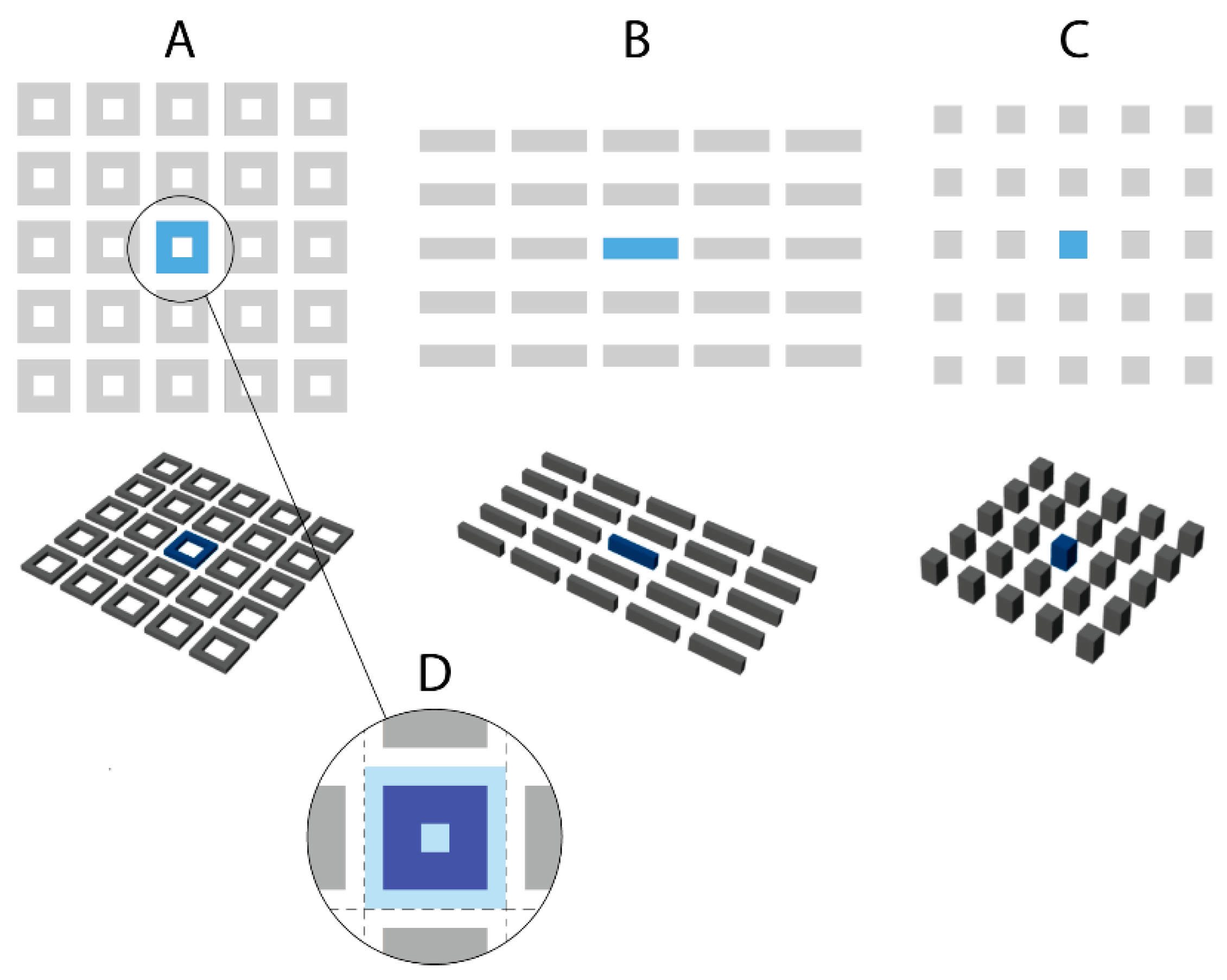
The selection of typical Swedish neighbourhood typologies for this study was conducted based on the existing Swedish residential stock of multi-family apartment blocks. Most of the Swedish residential stock (52%) consists of multi-dwelling buildings, and their proportion is increasing [23]. In the years 2011–2020, there were three times as many dwellings built as multi-family buildings than those of single- or double-dwelling building type. A survey into Swedish urban morphology revealed that the most prevalent multi-family building types can be reduced to courtyard, slab, and tower typologies [24]. In Malmö, slab and courtyard typologies appear to be the most dominant (Figure 1); other forms such as tower, L-shaped, and U-shaped exist but are less common. Although towers were found less frequently in Malmö, they appear more frequently in higher density cities, including the Swedish capital city, Stockholm. Thus, for this study, three neighbourhood typologies were selected for generating design iterations and further solar performance analysis: courtyard, slab, and tower (Figure 2A–C).
In order to facilitate the iterative modelling process, the neighbourhoods were modelled as homogeneous. Buildings within a neighbourhood were evenly spaced and arranged in a large, 5 × 5 unit orthogonal grid to include context shading (Figure 2A–C). Since the neighbourhoods were modelled homogenously, only the central building unit and the immediate area around it were analysed for solar access i.e., the middle unit was considered representative of the entire neighbourhood (Figure 2D). Vegetation and urban infrastructure were not included. Buildings were modelled without roof or façade details, which in digital city modelling is known as Level of Detail 1 (LoD1) [25]. The 3D models of design iterations were generated using Rhinoceros 7 [26] with Grasshopper [27].
Neighbourhood design iterations were created assuming ranges of geometrical design constraints. The dimensional constraints of the modelled neighbourhood geometries were intended to provide an adequate representation of the typical Swedish residential stock and a reasonable framework for the metric datasets. The discrete (countable) parameters are listed in Table 1, and the corresponding dimensions are marked in Figure 3. The number of design iterations changes in respect to the taxonomical class of calculated metrics; geometrical (G-) metrics have a smaller number of individual iterations because the building orientation variable is unapplicable for these metrics. Wall thickness (0.5 m) and storey height (3.0 m) were set as fixed values to calculate floor areas and space volumes. The plot offset was the distance from building façade edge facing outwards to the plot edge. For slab iterations, the offset distance was measured from the longer façade edge, and the distance from the short edge to the plot edge was equal to half the offset. This was found to be a common spatial feature in real slab neighbourhood cases.
The original dataset included more extreme cases (e.g., towers having 20 storeys and only 8 m span between buildings). However, iteration cases with a density indicator and a floor area ratio (FAR), larger than 4 were removed, as they represented highly unrealistic urban scenarios [28,29]. Even in the high-density city of New York, the maximum FAR averages 2.4 [30]. The FAR distribution of the original dataset is highly skewed (Figure 4). Neighbourhood design iterations with FAR above 4 were outliers of the dataset, as seen from the box plot in Figure 4. Removing the outliers provides a more balanced dataset.

2.2. Case Studies

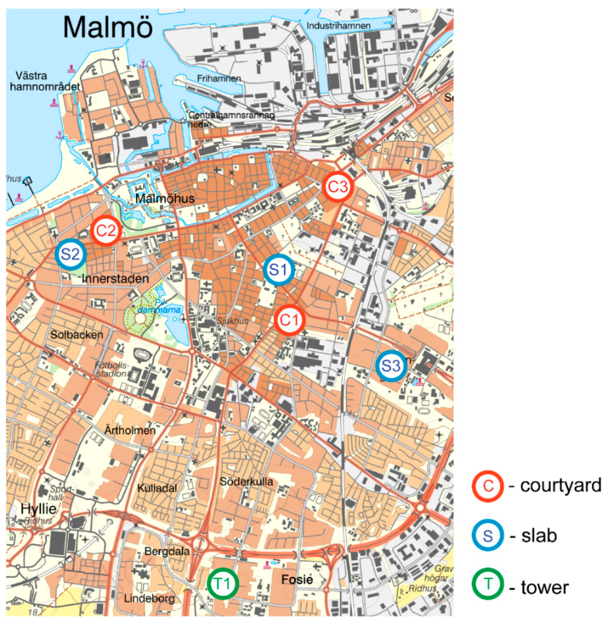
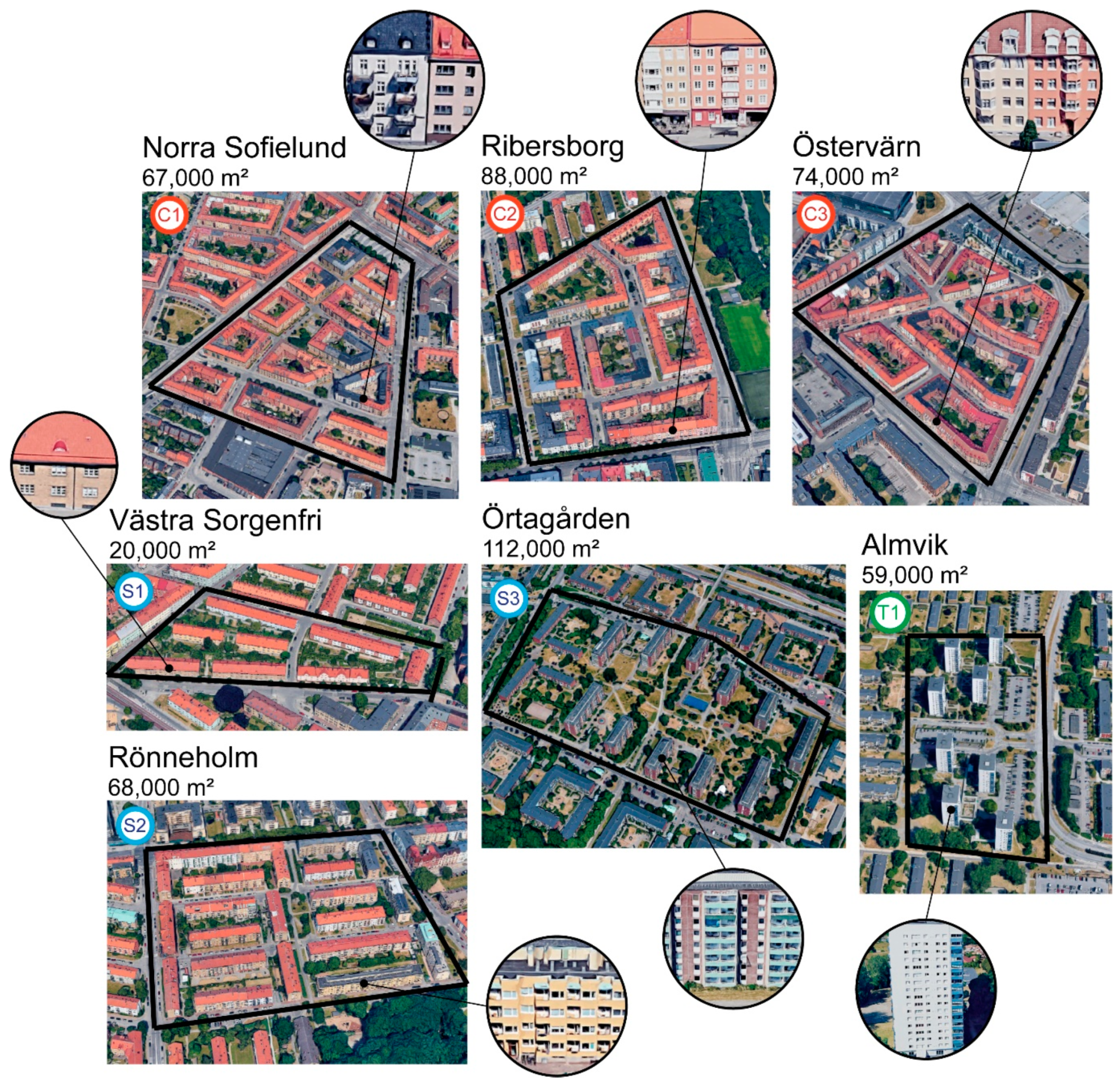
Case studies of seven existing neighbourhoods situated in Malmö, Sweden, were used to validate the iterative design datasets that were generated from hypothetical neighbourhoods (Section 2.1). The case studies were comprised of the same typologies as the iterations and included three courtyard neighbourhoods, three slab neighbourhoods, and one tower neighbourhood. The tower typology is underrepresented in the urban context of Malmö, therefore only one tower neighbourhood was included. The selected case studies are presented in Figure 5 and Figure 6.
The identification of suitable neighbourhood areas for case studies was governed by preassigned selection criteria. The definition of a neighbourhood is vague; many varying neighbourhood concepts exist, and the classification of the extents of one neighbourhood tends to be blurry. The concept of a “neighbourhood unit” was used in this paper as a framework for the identification of neighbourhood boundaries [31,32,33]. However, the factors that define a neighbourhood should remain flexible, diverse, and sensitive to the local context [34,35]. Swedish cities differ slightly from the West European cities as they developed in a more decentralized fashion, and they tend to be less densely populated [36]. They also seem to lack a precise definition of a neighbourhood [37]. The selection criteria were thus adapted to reflect the understanding of a neighbourhood in the Swedish context. The criteria were also intended to match the attributes assigned to the hypothetical neighbourhood design iterations in order to provide a suitable validation framework for the solar metrics. The following selection criteria were used:
  • The neighbourhood shall not be intersected by large traffic roads,
  • The neighbourhood must be comprised of residential multi-storey buildings and include one of the three analysed typologies (courtyard, slab, tower),
  • The neighbourhood shall be nearly homogenous (composed of the same typology),
  • The neighbourhood shall be surrounded by built context of similar height,
  • The case studies shall come from different administrative districts (sv: delområde).
The neighbourhoods were modelled in Rhinoceros 7. Geodata used for generating 3D models was obtained from Lantmäteriet [38]. The modelling details were similar to those of the iteration dataset: the geometries were simplified to LoD1, which means that roof and ground surfaces were horizontal and flat. Façade details, such as windows and balconies, were not included in the model, and neither were the vegetation and urban infrastructure elements.

2.3. Solar Performance Metrics

The selection of metrics for the analysis was based on an earlier review [18], and the metrics are listed in Table 2. All metrics belong to one of three classes of metrics: geometrical (G-metrics), latitudinal (L-metrics), and external climatic (EC-metrics). These three classes appear most suitable for solar assessments in urban planning stages due to the lower level of complexity compared with internal climatic metrics [18]. Only metrics with comparative and conforming functions [18] were used. Most of the metrics were sourced from previous literature, though there were also new metrics generated for this study; these were marked in Table 2 with an asterisk. Two types of urban surfaces were analysed for solar access depending on the assumed outdoor or indoor performance perspective, i.e., ground and facades (Figure 7). The analysis surfaces are given in the ‘Subject’ column of Table 2 and indicated with ‘G’ or ‘F’ suffix in metric acronyms. Roofs were not considered in this study because of their flat horizontal shape and the homogeneity of neighbourhood building heights in the iteration cases, which means that the roofs are receiving maximal solar access, and little variation due to design choices can be achieved. Metrics were simulated using Ladybug and Honeybee [39] in Grasshopper for Rhinoceros 7 [26].
G and L metrics that were calculated on façades (VSC, TH_F, ASH_F, RD_F) were simulated for a single string of points located on the façade at the height of 1.4 m and spaced 1 m apart (Figure 8), as solar access at the ground floor guarantees even better solar access at upper levels. Façade-based EC metrics measure surface irradiation, which affects the building’s overall thermal balance and solar energy potential, and thus, assessing the entire surface was deemed necessary to assess the radiation aspects. The radiation metrics were simulated for the entire façade surfaces (Figure 8).
There are different levels of site and layout factors that influence metrics, depending on their class, which are presented in Table 3. Location has impact on L- and EC-metrics; G-metrics are unaffected by location. Two European climates were investigated in the iterations analysis: Stockholm (59.65° N, 17.95° E) and Frankfurt (50.05° N, 8.60° E). Both locations belong to the transitional temperate zone of warm climate according to the classification by the European Environment Agency [40] yet are located at the northern and southern end of its reaches, which affects the amount of potential solar access. The case studies were simulated for the same locations. IWEC (international weather for energy calculations) EPW (energy plus weather) annual weather files were used for both Stockholm and Frankfurt [41].

2.4. Data Analysis

Metric datasets were analysed for correlations. The analysis method was two-fold: first, a Kendall correlation analysis was performed to assess the strength of associations based on its τB value, and then a pairwise graphical evaluation of metric relationships was conducted to assess the functions’ linearity and variance.
The datasets did not meet the necessary conditions for linear regression and Pearson correlation analyses. However, for those cases of pairwise metric relationships that resembled a linear function, Pearson correlation (r value) and linear regression analyses were conducted. These analyses were carried out for illustrative purposes and should be treated with caution since required assumptions were not met. Statistical analyses were performed in RStudio [42].
The suitability iteration-based datasets were validated by comparing them with case study datasets for each metric pair. The test hypothesis was that the slope and intercept of the iteration-based regression line of a given solar metric would fall within a 95% confidence interval (CI) of the slope and intercept ranges of the case studies.
Pre-analysis of simulated datasets indicated that it is sufficient to focus on only one climate location and analyse metric relationships for that climate. Thus, for the ease of analysis, Frankfurt was selected as the base climate for analysis and results presentation in this paper. All datasets from this study were made available for further inspection and reuse and were uploaded to a scientific data sharing repository [see the Data Availability Statement].

3. Results

3.1. Metric Correlation

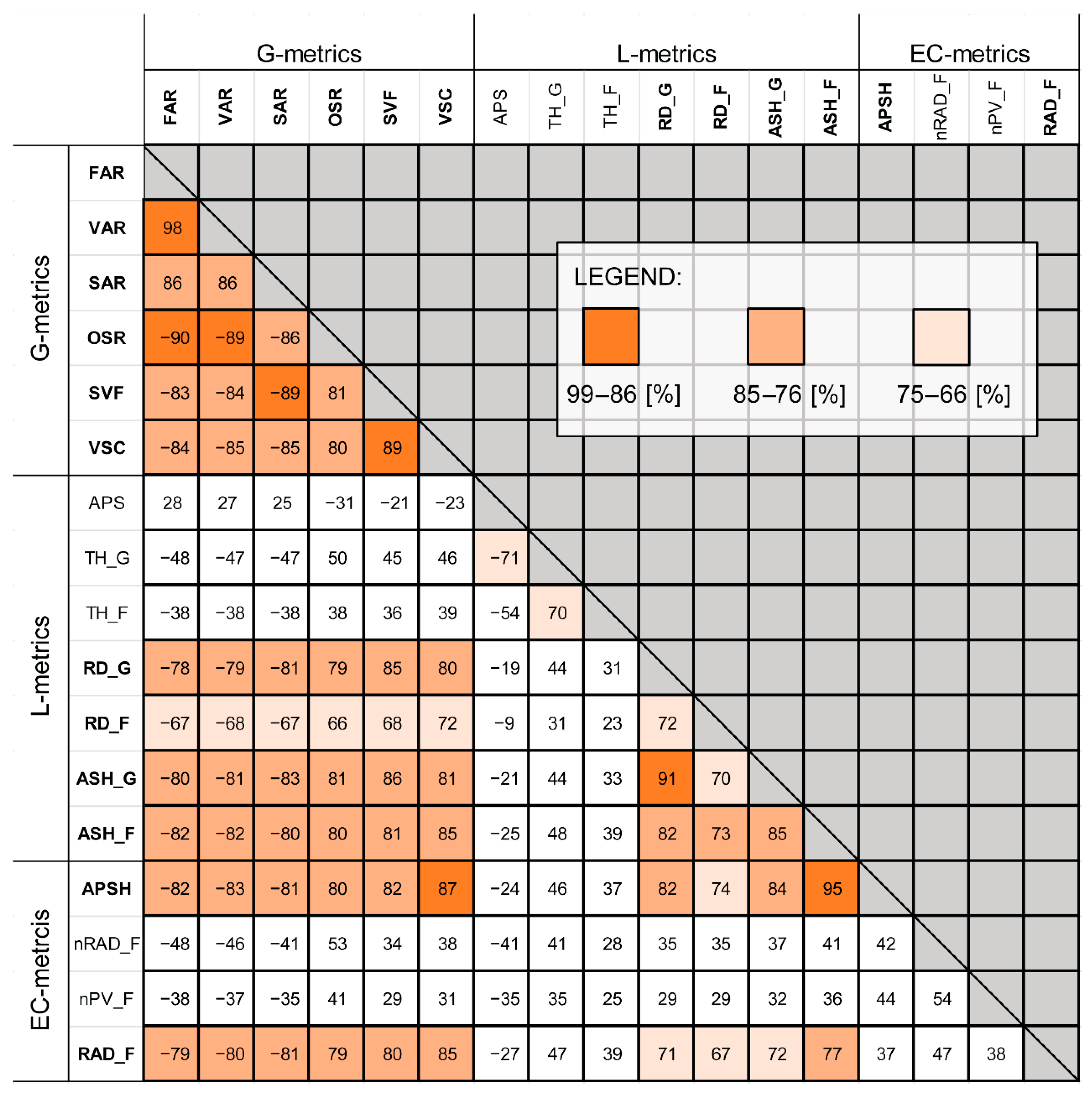
The results of the Kendall correlation analysis are presented in Figure 9. G-metrics show good correlation among themselves and with the comparative L- and EC-metrics. On the other hand, the correlation data hints that conforming metrics (metrics that are based on compliance to a threshold, e.g., pass/fail) do not correlate well with other metrics nor with each other. Furthermore, normalised radiation metrics did not prove high correlation to other metrics. The correlation study gave an initial indication of the strength of metrics’ pairwise relations, which allowed for the identification of metrics with high correlation scores for further graphical analysis and interpretation. In Figure 9, the high scoring metrics were highlighted (in bold).
Additionally, a Pearson correlation was conducted to examine the linearity of metric relationships. It indicated that functions of metric pairs FAR–VAR and SVF–VSC might be linear because in addition to the high Kendall correlation, their Pearson correlation results were also close to 1.

3.2. Urban Density

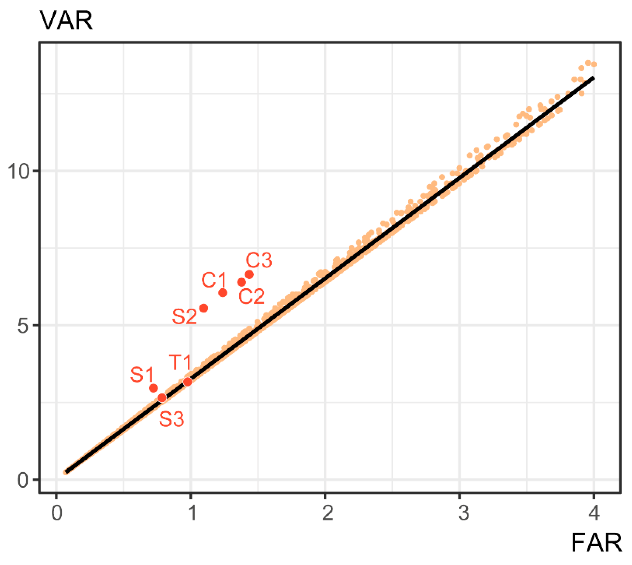
Two metrics pertaining to urban density were studied: FAR and VAR. They demonstrated a high Kendall correlation (τB = 0.98) and a potentially linear relationship (r = 1.00).
Figure 10 presents VAR as a function of FAR. The design iterations (black dots) show a nearly perfect linear function, while the case studies (red dots) diverge from the linear regression line. It is observed that the case studies do not fit the function well; that is because the case study storey heights varied, while storey height in design iterations was a constant.
Equation (1) explains the linear relationship between FAR and VAR, assuming that the storey height (hs) is constant.
VAR = FAR   ·   h s ,
Figure 10 suggests that VAR is a better indicator of urban density for assessing real neighbourhood examples for solar access because it is free of the independent variable: storey height. Indeed, FAR has been used in studies where urban density is an indirect indication of population density, such as in land or property value, and in transportation studies [30,43,44]. VAR might be a better indicator of urban density for solar access considerations because it pertains to volumes of buildings rather than population. Therefore, throughout this study, for the purpose of relating metrics to the urban density of the designs, the VAR metric was used as a density indicator.
Figure 11 presents the VAR iteration-based dataset distribution and the density of the case studies (blue dots). The iteration-based distribution is positively skewed. Although the case studies were randomly selected, their densities distribute roughly symmetrically on the opposite sides of the mean line and form two clusters. An explanation for this could be found in the consistency of spatial or temporal aspects in the urban planning practices in Malmö city.

3.3. G-Metrics

In this section, the results presented as metric datasets in graphs are identical for both simulated locations, Stockholm and Frankfurt, as G-metrics are only influenced by the geometry layout (see Table 3 in Section 2.3).
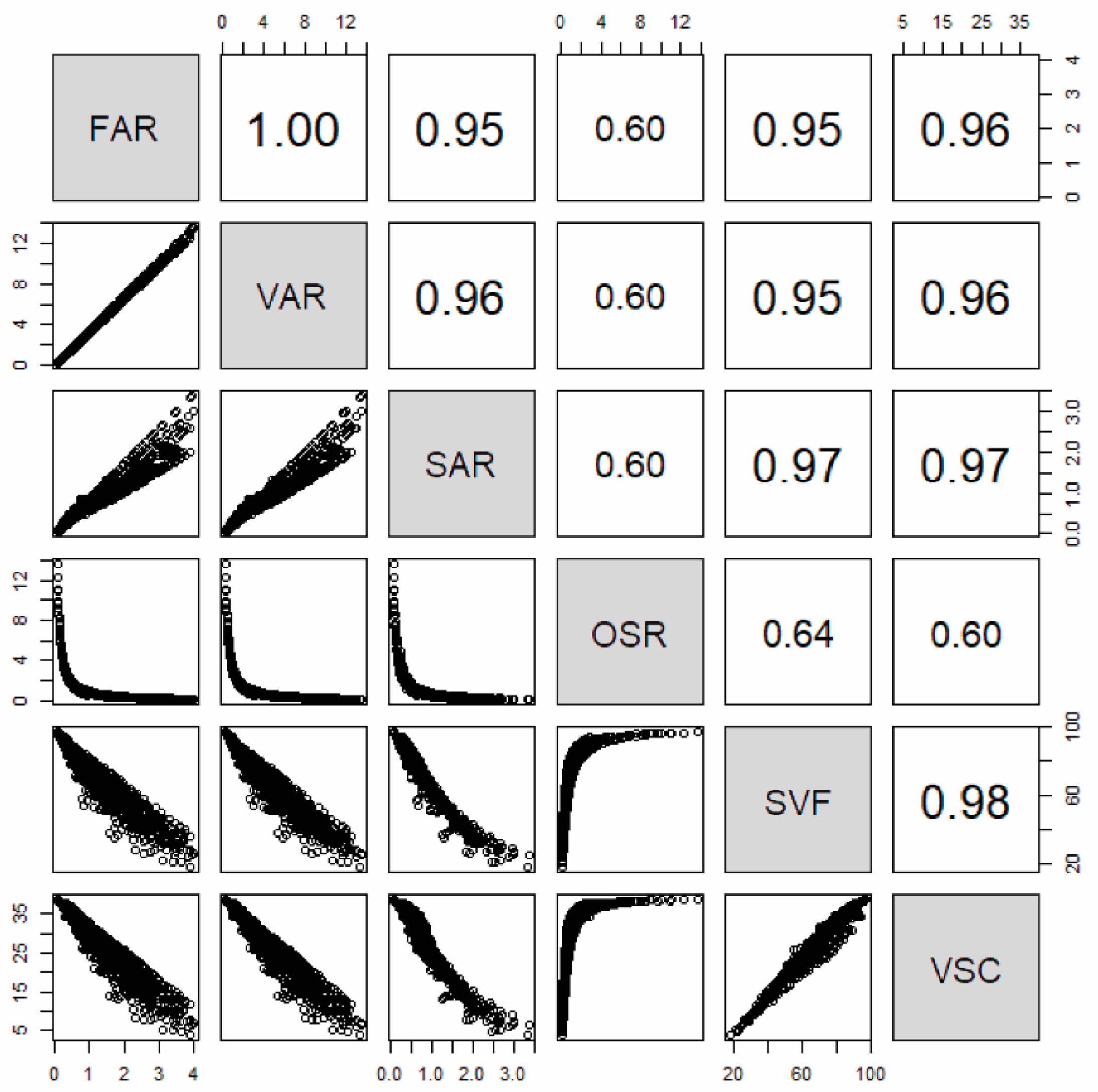
The G-metrics demonstrate a high Kendall correlation (Figure 9). The Pearson correlation analysis on these metrics resulted in equally high scores on the level of r ≈ 0.95, except for the OSR metric. Graphs in Figure 12, which display pairwise plots, show a nearly linear relationship for most of the G-metric pairs.
Among the morphological G-metrics, FAR, VAR, and SAR have similar correlation scores and appearance of graphs, which may indicate that they play a similar role in assessment and could be used interchangeably. SAR as a function of either of the density metrics, FAR or VAR, forms a fan-shaped data graph, meaning that the variance becomes larger the higher the metric values. The OSR metric, albeit having similar correlation scores, has a reciprocal graph shape. Since OSR is a ratio that takes similar inputs as FAR, it is considered inferior to FAR because of the unfavourable graph appearance.
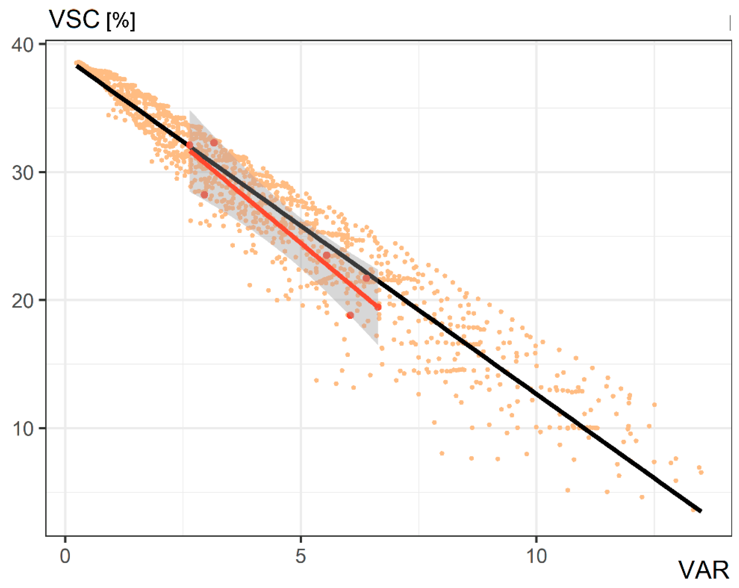
To further investigate the relationships between G-metrics, a linear regression analysis was conducted. Metrics SVF and VSC were tested against density VAR (Figure 13 and Figure 14) and against each other (Figure 15). The case studies fit well within the iteration-based datasets, as they appear close to the regression lines and within the simulated iterative designs. The graphs in Figure 13 and Figure 14 show fan-shaped relationships, which implies a heterogenous variance in the data. The SVF-VSC graph (Figure 15) shows a linear function with lower variance, though the function loses linearity at the data tails.

3.4. L-Metrics

L-metrics communicate solar access based on a set time period. The length of the reference time period affects the intensity of the computer simulation. To simplify the calculation, legislation normally recommends checking solar access for only a single reference day [45]. Looking at two L-metrics, RD_G and ASH_G, which were simulated at the ground surface but assume different time periods (reference day and a whole year), their graph shows linear characteristics (Figure 16). This relationship hints that the single-day-based RD_G metric may be used instead of the annually based ground ASH_G metric, which assumes a longer simulation period and thus takes more time to simulate. Additionally, the case studies regression line is nearly colinear with the iteration-based regression line, which validates the occurring relationship between RD_G and ASH_G.
The ground-based L-metrics (RD_G and ASH_G) show a non-linear relationship with density expressed by VAR (Figure 17). However, linear regression lines drawn for the case studies seem to approximate the respective parts of the iteration-based functions. In particular, the case studies regression line for the RD_G metric appears to be a close approximation of the original iteration-based trendline. Notably, graphs showing relation of density to ASH_G and RD_G have a similar shape (Figure 17), which is in line with their high mutual correlation and linear relationship in Figure 16.
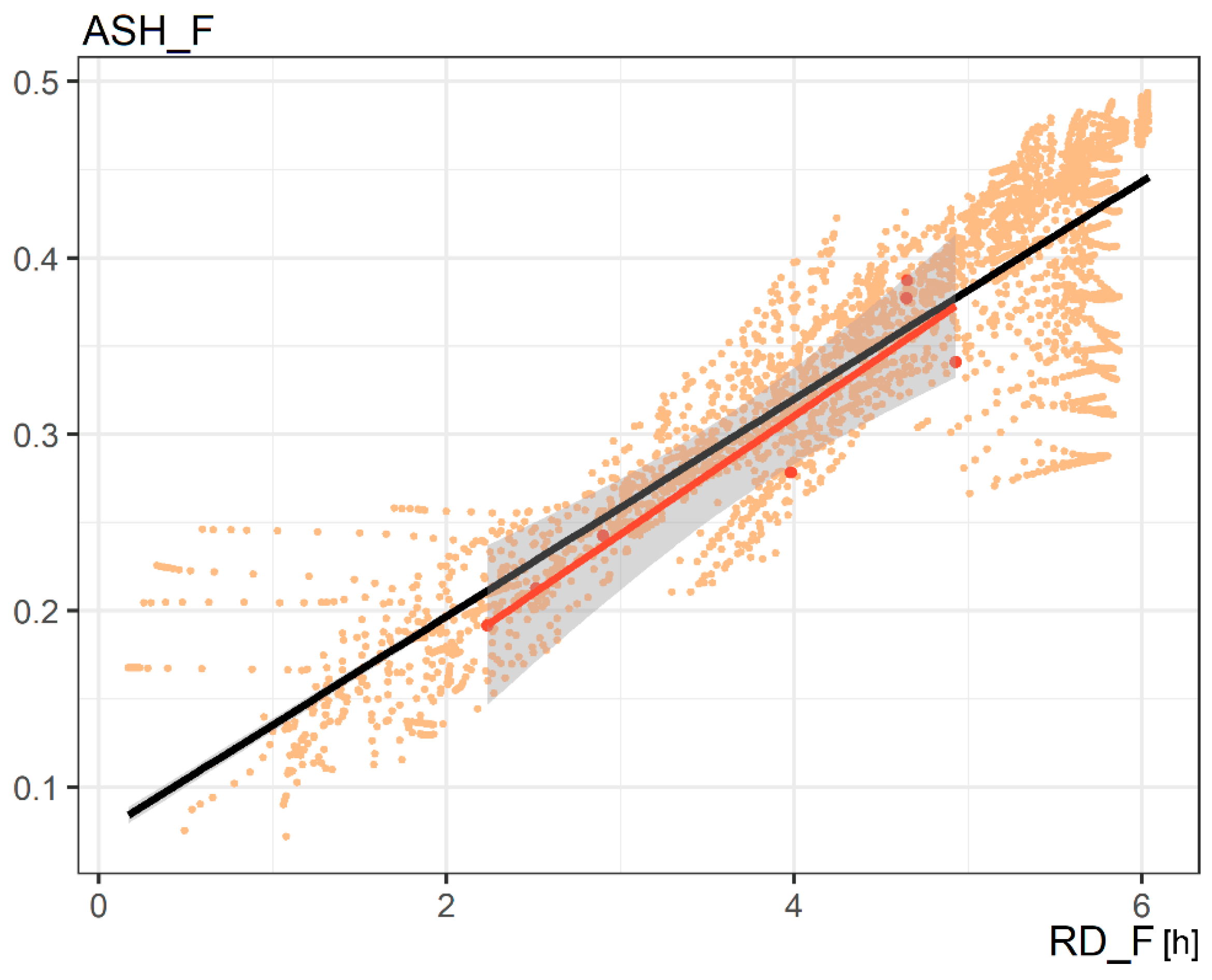
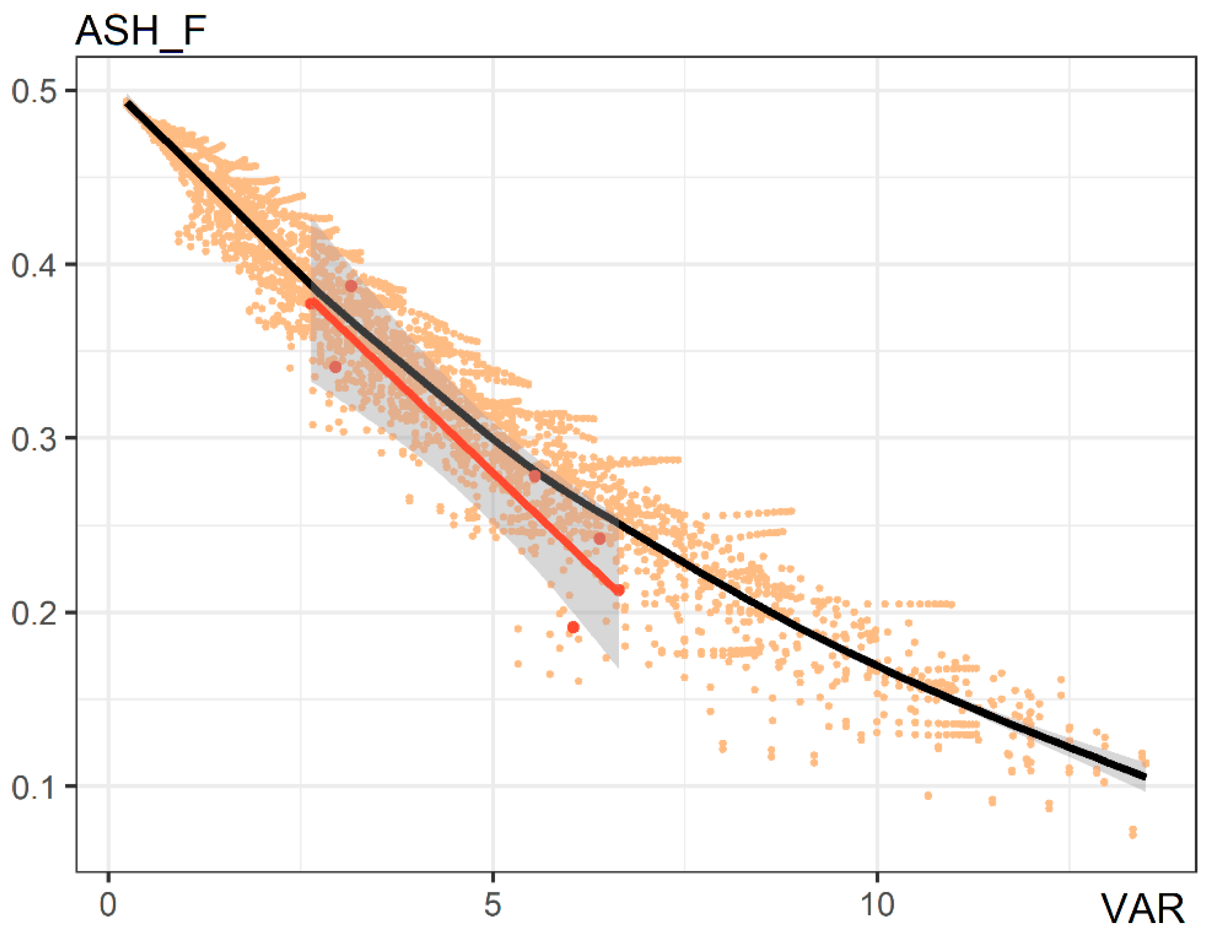
Looking at the same metrics (RD and ASH) but calculated for the facades, the relationship does not show the same high-definition linearity, and a larger variance is present in the datasets (Figure 18). Similarly, the relation of RD_F to VAR is dispersed and non-linear (Figure 19). The dispersion and lack of continuity in the data could be attributed to the orientation of the analysis surfaces. Facades are vertical surfaces, which see only half of the sky dome for any given façade orientation, as opposed to the ground surface, which sees the whole sky dome. For the iteration-based neighbourhood cases, four facades facing four different directions (right-angled) were considered. Slab typology is more sensitive to rotation because it has two lines of symmetry (the square courtyard and tower have four), and this sensitivity can be seen in the graph (Figure 19). Furthermore, RD_F is a simpler version of the direct sunlight hours metric and is only based on a single reference day (21 March), as opposed to the whole year in the calculation of ASH_F; the simulation uses 12 hourly solar vectors for calculation of the sunlight hours. The sparse number of vectors means that the measurement may lack continuity, as time is divided into few discrete intervals. This can create a stepwise appearance of the datasets in the graph. The difference is apparent when comparing the relationships of the two façade L-metrics (RD and ASH) to VAR (Figure 19 and Figure 20). The ASH_F metric not only shows higher correlation scores (Figure 9), but its relation graph also has a nearly linear data distribution (Figure 20), particularly for the lower densities.

3.5. EC-Metrics

APSH was the only metric in the EC-metric class that was not based on radiation; it was built on the hourly scores of the ASH_F metric with added information about cloud coverage, which was taken directly from the weather file. The correlation results for APSH (Figure 9) show almost identical scores as the simpler ASH_F metric. The correlation between ASH_F and APSH was at the level of 0.95, and their relationship was linear. This suggests that the simpler L-metric ASH_F may be used instead of the APSH, as there is no need to introduce an extra level of complexity with APSH.
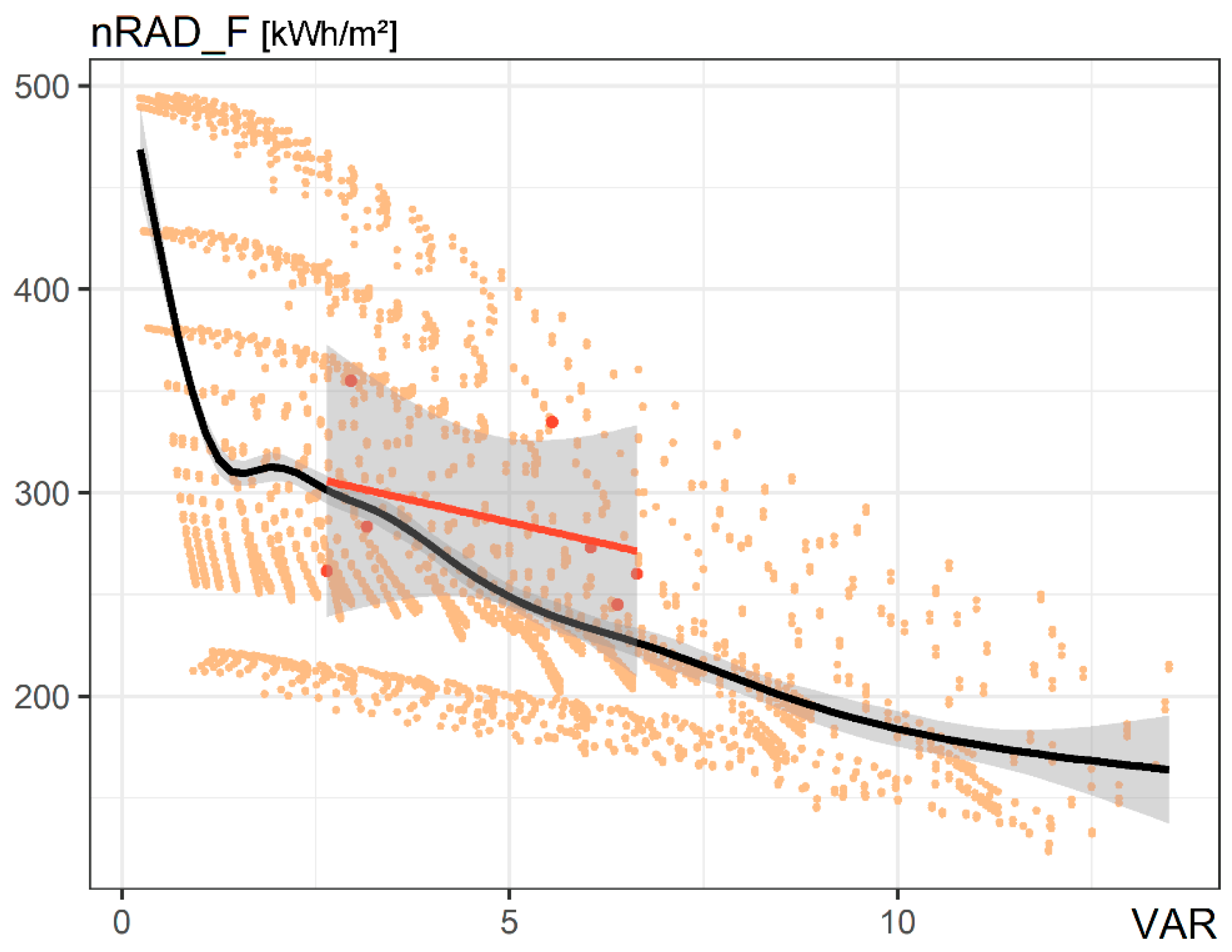
Figure 21 shows an example of how a graph with a normalized (in this case per floor area) or conforming (threshold based) radiation metric tends to look. The data distribution is scattered and clustered in a stepwise manner due to the initial discrete parameter settings. The normalized metrics also show low correlation levels with other metrics (Figure 9).
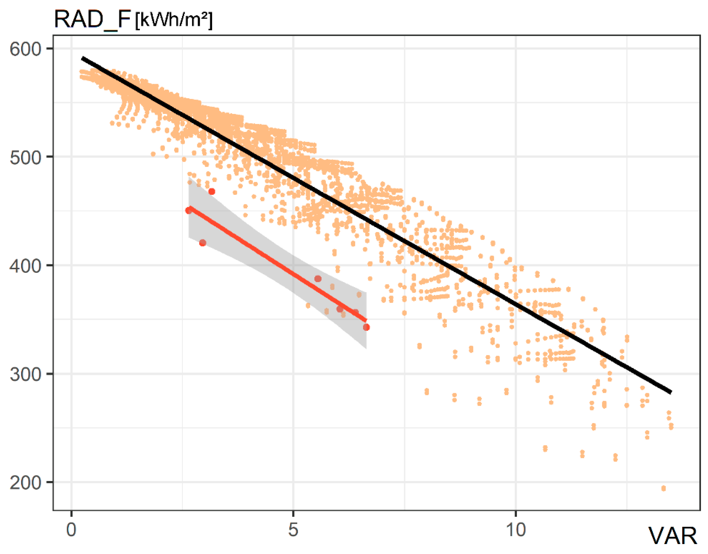
Considering the comparative façade radiation metric, RAD_F, the example pairwise graph in Figure 22 relating RAD_F metric with density shows that the case studies’ data points diverge from design iterations, as they scored significantly lower values of RAD_F. Façade irradiation was overestimated for the uniform, perfectly square, and evenly distributed neighbourhood typologies (iterations), while for the case studies, in which facades had non-right angles and more geometrical complexity, the scores were largely reduced. Compared with lower complexity metrics that were seen to have a good match between iterations and case studies, it seems that radiation metrics are more sensitive to changes in layout, surroundings, building forms and façade details. Furthermore, the lack of uniformity in building heights within case studies might have an additional impact on radiation estimates. The results suggest that, despite clearly defined curves of the iteration-based metric functions, these relationships do not hold for real neighbourhood cases.
Comparing the linear regression lines of the iterations and the case studies, it can be noted that their functions appear parallel. This may suggest that the regression lines based on the two datasets have a similar slope, just a different intercept (Figure 22). If the rate of change is similar, it may be justified to use the simpler metrics, such as VSC or ASH, to inform the selection of better performing designs. Although they might not be able to provide a precise estimation of radiation on facades, they may point towards designs that will provide a better radiation score in comparison to other proposals.
Table 4 presents 95% CIs of linear regression coefficients in some pairs of metrics. It confirms the observation on the regression slopes of the pairs containing the EC radiation metric. For all metrics pairs but the EC ones, the iteration-based CIs are narrower than the case study intervals (due to the higher number of degrees of freedom) and fall within the CIs of the case study regression coefficients. For those metrics pairs that include an EC metric, the intercept of the iteration-based cases does not fall within the case study interval, but the slope does. This means that the rate of change is expected to be the same, but the values will be reduced for more realistic neighbourhood geometries. The homogeneity of iteration design cases inflates the radiation results, and the CIs indicate an average reduction of 12% due to higher geometrical complexity. Reduction factors are typically applied for radiation estimates with urban designs of low LoD [46].

4. Discussion

This study showed that many simple metrics can potentially be suitable for solar evaluations at the urban planning stages due to good correlations. The solar access assessments may have varying objectives, and the two main paths of evaluation have been found to be the daylighting and sunlighting provision. For each of these assessment targets, the most suitable metrics were identified and listed in Table 5. Section 4.1 and Section 4.2 discuss the aspects of indoor and outdoor solar access assessments in relation to sunlight and daylight.

4.1. Solar Access Indoors

4.1.1. Daylight

The daylight factor (DF) is a common indicator of indoor daylighting. It is a G-metric, which means it is independent of location and climate inputs. The Swedish Building Code (SS-EN 17037) specifies that daylight in buildings should be measured using the DF metric simulated for a single point in a room [45]. The point, which is located halfway into the room from the aperture, 1 m away from the darkest wall, and 0.8 m above the ground, should score a DF of at least 1%. Driven by this legal constraint, urban planners in Sweden prioritise the daylighting objective when planning for solar access [16].
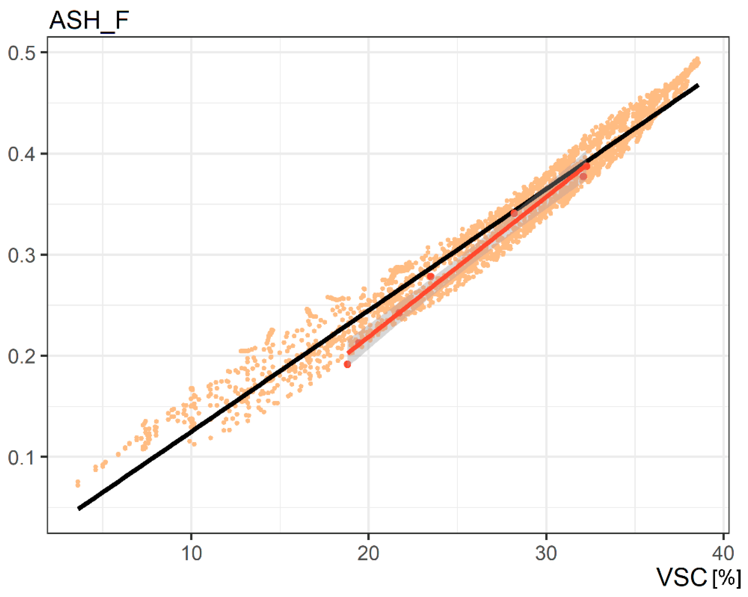
VSC can be used as an early indicator of daylighting at the façade level when aperture location and internal layouts are not yet established. Like the DF, the VSC is a G-metric, which is simulated for the CIE overcast sky model. The present study showed that the VSC correlates well with metrics of different complexities (e.g., Figure 14), also those which relate to sunlight (Figure 23). The Building Research Establishment (BRE) recommends a VSC level of at least 27% when conventional window design is used and cautions that a room with a VSC lower than 15% would likely need large windows to ensure good daylighting [47]. BRE states that VSC levels between 15% and 27% may provide enough daylighting if proper layout and fenestration design strategies are applied. However, it is important to note that the recommended VSC levels were given for the UK context, where national daylighting requirements are not mandated (BS-EN 17037 was withdrawn). It is thus yet uncertain how these recommended VSC levels would translate to meet the Swedish daylighting requirements.
The VSC metric dataset created in this study can be used to guide urban planners towards good daylight potential. We suggest two alternative methods to apply this dataset in practice, which are derived from a fixed variable: urban density as VAR. This means that, prior to the assessments, urban planning authorities must decide on the planned population density of a developed area. Assuming the amount of occupied floor area per inhabitant, the population density can be translated into urban density e.g., VAR. Knowing the target range of VAR, urban planners may use the simulated VSC dataset to retrieve a list of possible design cases from highest to lowest performing ones for the assigned density (Figure 24). Further on, introducing the area of the developed plot, the list can be reduced to include only those cases that fit a given plot (Figure 24). Alternatively, the method can provide urban planners with a range of expected VSC values to inform their design (Figure 25). In this case, the urban planners must perform VSC analysis themselves, and then use the VSC range as a guiding tool. It is important to mark that the method is intended for comparative design assessments, i.e., to determine which design proposals perform best, and not to accurately predict performance scores. This is future work which requires the identification of value benchmarks for performance levels backed by empirical evidence.

4.1.2. Sunlight

Access to direct sunlight in dwellings in Sweden is acknowledged in building legislation; however, it is not regulated as strictly as daylight. The Swedish Building Regulations [48] state that a minimum one room in a dwelling which people frequent more than occasionally should have access to sunlight, but how this should be enforced or measured is not specified. The European Daylighting Standard [45], on the other hand, provides a more concrete assessment method. It uses an L-metric, direct sunlight hours, calculated for a point on the façade and for a single reference day between 1 February and 21 March. The exposure-to-sunlight levels are given from minimum: 1.5 h, through medium: 3 h, to maximum: 4 h. The European Standard sunlight metric is thus of conforming function, using a time constraint of one day. The stated sunlight stipulation is thus far just a recommendation.
The results of this study showed that some metrics have lower correlation to other solar metrics, and their pairwise relationships may have a dispersed appearance. Thus, may be less suitable for early assessment purposes. In particular, the conforming metrics were poorly correlated with other metrics, presenting high variance and lack of order in the data. Furthermore, the comparison of façade-based sunlight metrics, ASH_F and RD_F (Figure 18) was favourable to the annual time constraint, as it provides higher correlations, more continuous relationships with other metrics, and better linearity (Figure 20 and Figure 23). The present study showed that the single-day RD_F metric has a large variance in the data in relation to other metrics. Current sunlight recommendations are based on a single day metric, and the present study showed that this time constraint may be less suitable in assessments due to the directionality of façade surfaces and a low number of simulated solar vectors. As a result of that, for example, the recommendation disqualifies dwellings from having all habitable rooms directly facing the North. There is insufficient evidence regarding user preferences with regard to solar access. These considerations may call into question the current assessment method for sunlight exposure, which is based on a poorly correlated conforming and single-day-based metric.
Conforming metrics, albeit their poor correlation, play an important role in assessments and should not be discounted. However, to apply design criteria using fixed thresholds with confidence, datasets need to have assigned evidence-based benchmarks, and the evidence on the amount of sunlight needed is currently lacking. More technical- and observation-based evidence on solar access at the façade level is needed in support of sustainable design objectives.

4.2. Solar Access Outdoors

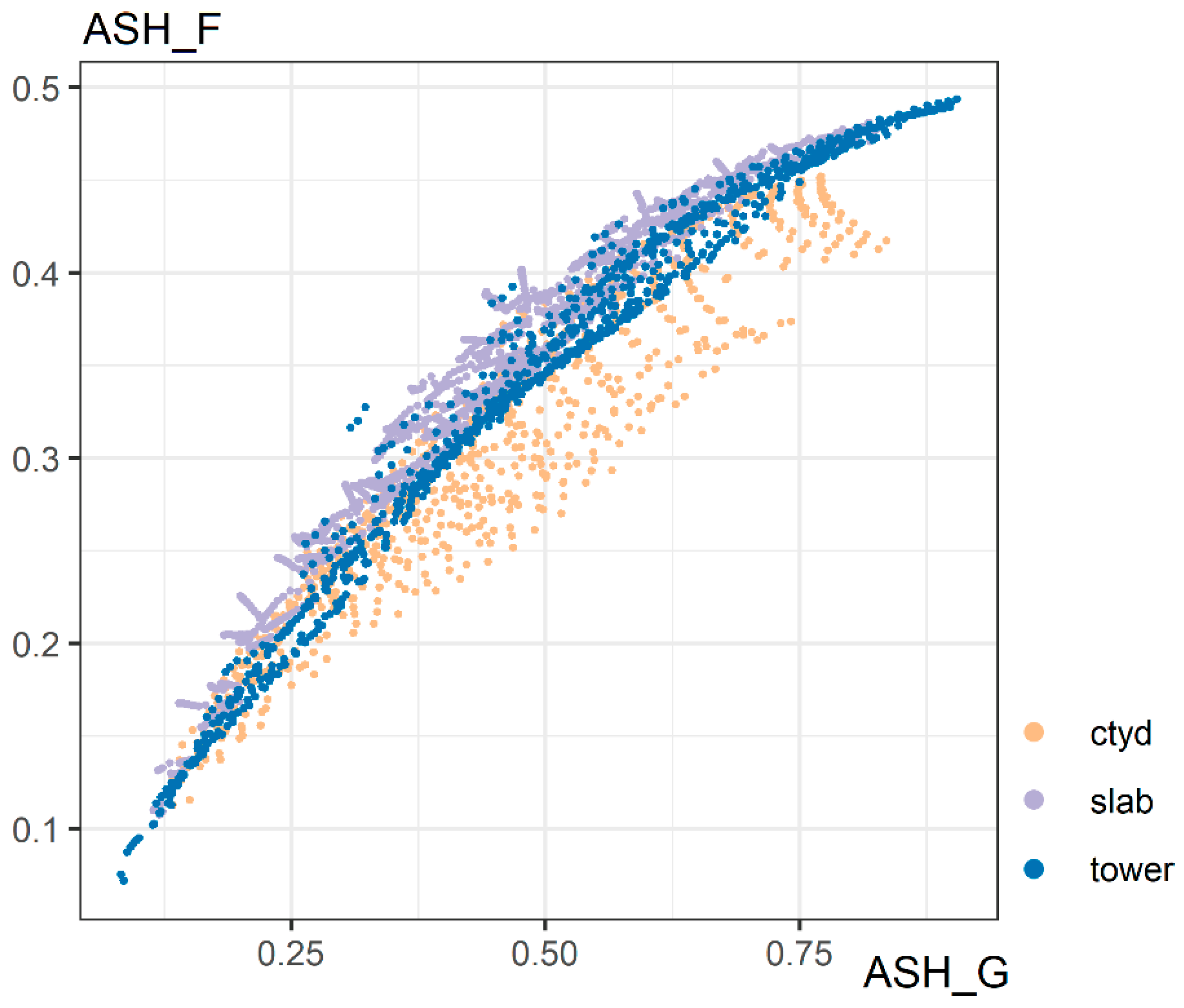
Solar access in urban settings is often assessed at the outdoor ground level for visualization purposes (e.g., shadowing on the ground), but it has not yet been legislated. Ensuring solar access outdoors may be important for wellbeing, energy applications, and greenery growth. The results of this study showed that there is a good correlation and linear relationship between façade-based and ground-based G-metrics, i.e., VSC and SVF (Figure 15). Similarly, there is a strong correlation between ASH on the ground (ASH_G) and ASH at the façade level (ASH_F) (Figure 26). An interpretation of this result is that the indication of performance quality obtained from analysing only one type of target surface, either ground or façade, may be applicable to both indoor and outdoor environments.
The provision of solar access outdoors is also important in the aspects of urban heat island and microclimate. This study suggests that SVF is a promising early design indicator of daylighting performance of outdoor solar access. Since SVF has been previously linked to urban heat island mitigation [49], it strengthens the argument for implementing this metric into early solar access evaluations. Future work should establish limiting values for outdoor solar access SVF recommendations relative to the mitigation of the unwanted heat retention in cities.
An example of how the ground- and façade-based solar access data may be used in urban design assessments is presented in Figure 27. There are differences between different typologies depending on the target analysis surface used. The comparative solar performance graphs may be used as a tool to inform urban planners about the differences in performance of certain typologies and the trade-offs when considering different objectives. Currently, due to the legislative emphasis on the indoor environment, the priority in design assessments might be given to those typologies that score better solar access metrics at the façade level, e.g., slab; however, if significance was given to solar access outdoors, the courtyard typology could be more preferable.

4.3. Limitations and Future Work

This study was limited to particular neighbourhood typologies. The prerequisites for the selection of neighbourhood case studies, as well as the assumptions for modelling neighbourhood design iterations, gave constraints to the resulting metric datasets. In the future, these datasets could be expanded by adding neighbourhood cases of a wider variety, including diverse typologies and non-homogenous designs. A more complete database of solar metrics will support the decision-making process and improve solar-driven urban planning assessment methods, such as the two alternative approaches suggested in Section 4.1.1. An extended database could also open up possibilities for more advanced prediction models based on data statistics and machine learning.
The study focused on the European climates, and the solar performance metrics were selected assuming the northern latitude context for performance assessments. The solar access design objectives of northern locations may differ for other climates; for instance, in the hot climate regions, sunlight might be considered a liability, and access to it may have to be restricted in the design planning. The effect of different climates and latitudes should be studied further to also consider the impact of solar access on the microclimate.
Some metrics in this paper were calculated as an average value for the entire analysis area. This kind of assessment may be simplifying and reducing the design performance score. In some cases, in design assessments, it may be more valuable to have the metric displayed visually over the entire analysis area in order to be able to check for critical spots, especially in case of a non-homogenous neighbourhood.
Future work should establish relevant performance benchmarks for the suitable metrics that were presented in this study. Another point of perspective is also needed: occupants’ perception of sunlight, both indoors and outdoors. There is scarce empirical evidence to support existing recommendations. This input will be instrumental in creating holistic methods of solar access evaluation, as it can help establish solar access targets assuming wellbeing as one of the urban design drivers alongside energy sustainability.

5. Conclusions

This study evaluated solar performance metrics, their graphical relations, and statistical correlations. The study was based on homogenous neighbourhood designs and focused on the context of northern Europe. The neighbourhood designs were validated via comparison with six case studies.
The outcomes of this study suggest that simple geometrical and latitudinal metric classes are valid candidates for potential solar performance indicators in the urban planning level of building design stages, whereas the external climatic metrics deem too complex. It was shown that, in some cases, the simpler metrics are even better suited for evaluating the performance of simple building blocks, i.e., the level of detail used in the early urban planning stage. More complex metrics were indeed more sensitive to geometrical details of the urban models and building facades.
In particular, it is concluded that VSC and SVF (for daylighting) and ASH_F and RD_G (for sunlighting) are good candidate metrics for describing solar access indoors and outdoors, respectively.
The urban design and metric database created in this study may be useful for establishing assessment paradigms and prediction models. The database of metric values can be used in solar assessments of urban designs, may be used in prediction models, and can be of interest for future studies involving design optimization using advanced machine learning techniques. More diverse design solutions may be added to the datasets for increased validity and reliability. Some examples of urban-level solar assessment methods applying appropriate metrics specific for a given solar design objective were presented in this study.
Selecting appropriate metric thresholds is a challenge for the next phases of research into solar performance indicators. Performance benchmarks should be supported by evidence-based research, balancing energy and wellbeing objectives of sustainable neighbourhoods.

Author Contributions

Conceptualization, A.C., N.G., J.K. and M.W.; methodology, A.C., N.G., J.K. and M.W.; software, A.C.; validation, A.C., N.G., J.K. and M.W.; formal analysis, A.C.; investigation, A.C.; resources, J.K. and M.W.; data curation, A.C.; writing—original draft preparation, A.C.; writing—review and editing, A.C., N.G., J.K. and M.W.; visualization, A.C.; supervision, N.G., J.K. and M.W.; project administration, J.K. and M.W.; funding acquisition, M.W. and J.K. All authors have read and agreed to the published version of the manuscript.

Funding

This research was funded by the Swedish Energy Agency (Energimyndigheten)—grant number 49518-1.

Data Availability Statement

The data presented in this study are openly available in the Swedish National Data Service at https://doi.org/10.5878/jf63-ay82 (accessed on 30 August 2022), reference number SND-ID: 2022-137.

Acknowledgments

This project contributes to the International Energy Agency Solar Heating & Cooling programme (IEA SHC) Task 63 “Solar Neighborhood Planning”. The authors wish to acknowledge the experts in IEA SHC Task 63 for the fruitful discussions during the Task activities.

Conflicts of Interest

The authors declare that they have no conflict of interest.

References

  1. Littlefair, P. Passive Solar Urban Design: Ensuring the Penetration of Solar Energy into the City. Renew. Sustain. Energy Rev. 1998, 2, 303–326. [Google Scholar] [CrossRef]
  2. Beckers, B. Solar Energy at Urban Scale; John Wiley and Sons: Hoboken, NJ, USA, 2013; ISBN 9781848213562. [Google Scholar]
  3. Knowles, R.L. The Solar Envelope: Its Meaning for Energy and Buildings. Energy Build. 2003, 35, 15–25. [Google Scholar] [CrossRef]
  4. IEA SHC. Task 51 Solar Energy in Urban Planning. In Approaches, Methods and Tools for Solar Energy in Urban Planning; IEA SHC: Cedar, MI, USA, 2018. [Google Scholar]
  5. Peronato, G.; Rastogi, P.; Rey, E.; Andersen, M. A Toolkit for Multi-Scale Mapping of the Solar Energy-Generation Potential of Buildings in Urban Environments under Uncertainty. Sol. Energy 2018, 173, 861–874. [Google Scholar] [CrossRef]
  6. Sarralde, J.J.; Quinn, D.J.; Wiesmann, D.; Steemers, K. Solar Energy and Urban Morphology: Scenarios for Increasing the Renewable Energy Potential of Neighbourhoods in London. Renew. Energy 2015, 73, 10–17. [Google Scholar] [CrossRef]
  7. Bilu, C.; Einat, H.; Zimmet, P.; Vishnevskia-Dai, V.; Kronfeld-Schor, N. Beneficial Effects of Daytime High-Intensity Light Exposure on Daily Rhythms, Metabolic State and Affect. Sci. Rep. 2020, 10, 19782. [Google Scholar] [CrossRef] [PubMed]
  8. Knoop, M.; Stefani, O.; Bueno, B.; Matusiak, B.; Hobday, R.; Wirz-Justice, A.; Martiny, K.; Kantermann, T.; Aarts, M.P.J.; Zemmouri, N.; et al. Daylight: What Makes the Difference? Light. Res. Technol. 2020, 52, 423–442. [Google Scholar] [CrossRef]
  9. Holick, M.F. Sunlight and Vitamin D for Bone Health and Prevention of Autoimmune Diseases, Cancers, and Cardiovascular Disease. Am. J. Clin. Nutr. 2004, 80, 1678S–1688S. [Google Scholar] [CrossRef] [PubMed]
  10. Fahimipour, A.K.; Hartmann, E.M.; Siemens, A.; Kline, J.; Levin, D.A.; Wilson, H.; Betancourt-Román, C.M.; Brown, G.; Fretz, M.; Northcutt, D.; et al. Daylight Exposure Modulates Bacterial Communities Associated with Household Dust. Microbiome 2018, 6, 175. [Google Scholar] [CrossRef]
  11. United Nations-Department of Economic and Social Affairs-Population Division. World Urbanization Prospects. The 2018 Revision; United Nations: New York, NY, USA, 2019. [Google Scholar]
  12. Angel, S.; Lamson-Hall, P.; Blei, A.; Shingade, S.; Kumar, S. Densify and Expand: A Global Analysis of Recent Urban Growth. Sustainability 2021, 13, 3835. [Google Scholar] [CrossRef]
  13. Bournas, I.; Dubois, M.-C. Daylight Regulation Compliance of Existing Multi-Family Apartment Blocks in Sweden. Build. Environ. 2019, 150, 254–265. [Google Scholar] [CrossRef]
  14. Kanters, J.; Wall, M. Experiences from the Urban Planning Process of a Solar Neighbourhood in Malmö, Sweden. Urban Plan. Transp. Res. 2018, 6, 54–80. [Google Scholar] [CrossRef]
  15. Lobaccaro, G.; Croce, S.; Lindkvist, C.; Munari Probst, M.C.; Scognamiglio, A.; Dahlberg, J.; Lundgren, M.; Wall, M. A Cross-Country Perspective on Solar Energy in Urban Planning: Lessons Learned from International Case Studies. Renew. Sustain. Energy Rev. 2019, 108, 209–237. [Google Scholar] [CrossRef]
  16. Kanters, J.; Gentile, N.; Bernardo, R. Planning for Solar Access in Sweden: Routines, Metrics, and Tools. Urban Plan. Transp. Res. 2021, 9, 348–368. [Google Scholar] [CrossRef]
  17. Nault, E.; Peronato, G.; Rey, E.; Andersen, M. Review and Critical Analysis of Early-Design Phase Evaluation Metrics for the Solar Potential of Neighborhood Designs. Build. Environ. 2015, 92, 679–691. [Google Scholar] [CrossRef]
  18. Czachura, A.; Kanters, J.; Gentile, N.; Wall, M. Solar Performance Metrics in Urban Planning: A Review and Taxonomy. Buildings 2022, 12, 393. [Google Scholar] [CrossRef]
  19. Morganti, M.; Salvati, A.; Coch, H.; Cecere, C. Urban Morphology Indicators for Solar Energy Analysis. Energy Procedia 2017, 134, 807–814. [Google Scholar] [CrossRef]
  20. Shi, Z.; Fonseca, J.A.; Schlueter, A. A Parametric Method Using Vernacular Urban Block Typologies for Investigating Interactions between Solar Energy Use and Urban Design. Renew. Energy 2021, 165, 823–841. [Google Scholar] [CrossRef]
  21. Zhang, J.; Heng, C.K.; Malone-Lee, L.C.; Hii, D.J.C.; Janssen, P.; Leung, K.S.; Tan, B.K. Evaluating Environmental Implications of Density: A Comparative Case Study on the Relationship between Density, Urban Block Typology and Sky Exposure. Autom. Constr. 2012, 22, 90–101. [Google Scholar] [CrossRef]
  22. Chen, K.W.; Norford, L. Evaluating Urban Forms for Comparison Studies in the Massing Design Stage. Sustainability 2017, 9, 987. [Google Scholar] [CrossRef]
  23. Statistics Sweden (SCB) Nearly 5.1 Million Dwellings in Sweden. Available online: https://www.scb.se/en/finding-statistics/statistics-by-subject-area/housing-construction-and-building/housing-construction-and-conversion/dwelling-stock/pong/statistical-news/dwelling-stock-december-31-2021/ (accessed on 10 May 2022).
  24. Rådberg, J.; Friberg, A. Svenska Stadstyper: Historik, Exempel, Klassificering; Kungliga tekniska högskolan, Institutionen för arkitektur och stadsbyggnad: Stockholm, Sweden, 1996; ISBN 9171706992. [Google Scholar]
  25. Nouvel, R.; Schulte, C.; Eicker, U.; Pietruschka, D.; Coors, V. CityGML-Based 3D City Model for Energy Diagnostics and Urban Energy Policy Support. In Proceedings of the BS2013: 13th Conference of International Building Performance Simulation Association, Chambéry, France, 26–28 August 2013; pp. 218–225. [Google Scholar]
  26. McNeel, R. Associates Rhinoceros 3D, Version 7. Available online: https://www.rhino3d.com/ (accessed on 6 December 2021).
  27. McNeel, R. Associates Grasshopper—Algorithmic Modeling for Rhino. 2022. Available online: https://www.grasshopper3d.com/?overrideMobileRedirect=1 (accessed on 6 December 2021).
  28. American Society of Planning Officials. Information Report No. 111: Floor Area Ratio; American Society of Planning Officials: Chicago, IL, USA, 1958. [Google Scholar]
  29. Krehl, A.; Siedentop, S.; Taubenböck, H.; Wurm, M.; Behnisch, M.; Meinel, G.; Kainz, W. A Comprehensive View on Urban Spatial Structure: Urban Density Patterns of German City Regions. ISPRS Int. J. Geo-Inf. 2016, 5, 76. [Google Scholar] [CrossRef] [Green Version]
  30. Moon, B. The Effect of FAR (Floor Area Ratio) Regulations on Land Values: The Case of New York. Pap. Reg. Sci. 2019, 98, 2343–2354. [Google Scholar] [CrossRef]
  31. Perry, C. The Neighborhood Unit: A Scheme of Arrangement for the Family-Life Community. In The Regional Plan of New York and Its Environs; Russell Sage Foundation: New York, NY, USA, 1929; Volume VII, ISBN 9781136205668. [Google Scholar]
  32. Mumford, L. The Neighborhood and the Neighborhood Unit. Town Plan. Rev. 1954, 24, 256–270. [Google Scholar] [CrossRef]
  33. Mehaffy, M.W.; Porta, S.; Romice, O. The “Neighborhood Unit” on Trial: A Case Study in the Impacts of Urban Morphology. J. Urban 2015, 8, 199–217. [Google Scholar] [CrossRef]
  34. Byun, N.; Choi, Y.; Choi, J. Neighborhood Unit: Effective or Obsolete? J. Asian Archit. Build. Eng. 2014, 13, 617–624. [Google Scholar] [CrossRef]
  35. Olson, P. Urban Neighborhood Research: Its Development and Current Focus. Urban Aff. Rev. 1982, 17, 491–518. [Google Scholar] [CrossRef]
  36. Gallion, A.B.; Eisner, S. The Urban Pattern: City Planning and Design, 5th ed.; Van Nostrand Reinhold: New York, NY, USA, 1985; ISBN 0442227310. [Google Scholar]
  37. Dahlberg, G.-B.; Ödmann, E. Stadsutveckling Och Planering i Sverige; Läromedelsförl. i samverkan med Byggforskningen; T/Statens råd för byggnadsforskning: Stockholm, Sweden, 1969. [Google Scholar]
  38. Lantmäteriet Geodataportalen. Available online: https://www.lantmateriet.se/sv/geodata/Geodataportalen/ (accessed on 30 August 2022).
  39. Ladybug Tools Ladybug Tools|Home Page. Available online: https://www.ladybug.tools/ (accessed on 11 October 2021).
  40. European Environment Agency (EEA). Main Climates of Europe. Available online: https://www.eea.europa.eu/data-and-maps/figures/climate (accessed on 30 August 2022).
  41. ASHRAE. International Weather for Energy Calculations (IWEC Weather Files) Users Manual and CD-ROM; ASHRAE: Atlanta, GA, USA, 2001. [Google Scholar]
  42. RStudio Team. RStudio: Integrated Development Environment for R; RStudio, PBC: Boston, MA, USA, 2021. [Google Scholar]
  43. Joshi, K.K.; Kono, T. Optimization of Floor Area Ratio Regulation in a Growing City. Reg. Sci. Urban Econ. 2009, 39, 502–511. [Google Scholar] [CrossRef]
  44. Kono, T.; Kusum Joshi, K. A New Interpretation on the Optimal Density Regulations: Closed and Open City. J. Hous. Econ. 2012, 21, 223–234. [Google Scholar] [CrossRef]
  45. SSI. CEN SS-EN 17037:2018+A1:2021; Daylight in Buildings. Swedish Standards Institute: Stockholm, Sweden, 2021.
  46. Lobaccaro, G.; Lisowska, M.M.; Saretta, E.; Bonomo, P.; Frontini, F. A Methodological Analysis Approach to Assess Solar Energy Potential at the Neighborhood Scale. Energies 2019, 12, 3554. [Google Scholar] [CrossRef]
  47. Littlefair, P.J.; King, S.; Howlett, G.; Ticleanu, C.; Longfield, A. Site Layout Planning for Daylight and Sunlight (BR 209), 3rd ed.; S&P Global: New York, NY, USA, 2022; ISBN 978-1-84806-483-6. [Google Scholar]
  48. Boverket. Boverkets Byggregler (BFS 2019:2)—Föreskrifter Och Allmänna Råd; Boverket: Karlskrona, Sweden, 2011. [Google Scholar]
  49. Oke, T.R. Canyon Geometry and the Nocturnal Urban Heat Island: Comparison of Scale Model and Field Observations. J. Climatol. 1981, 1, 237–254. [Google Scholar] [CrossRef]
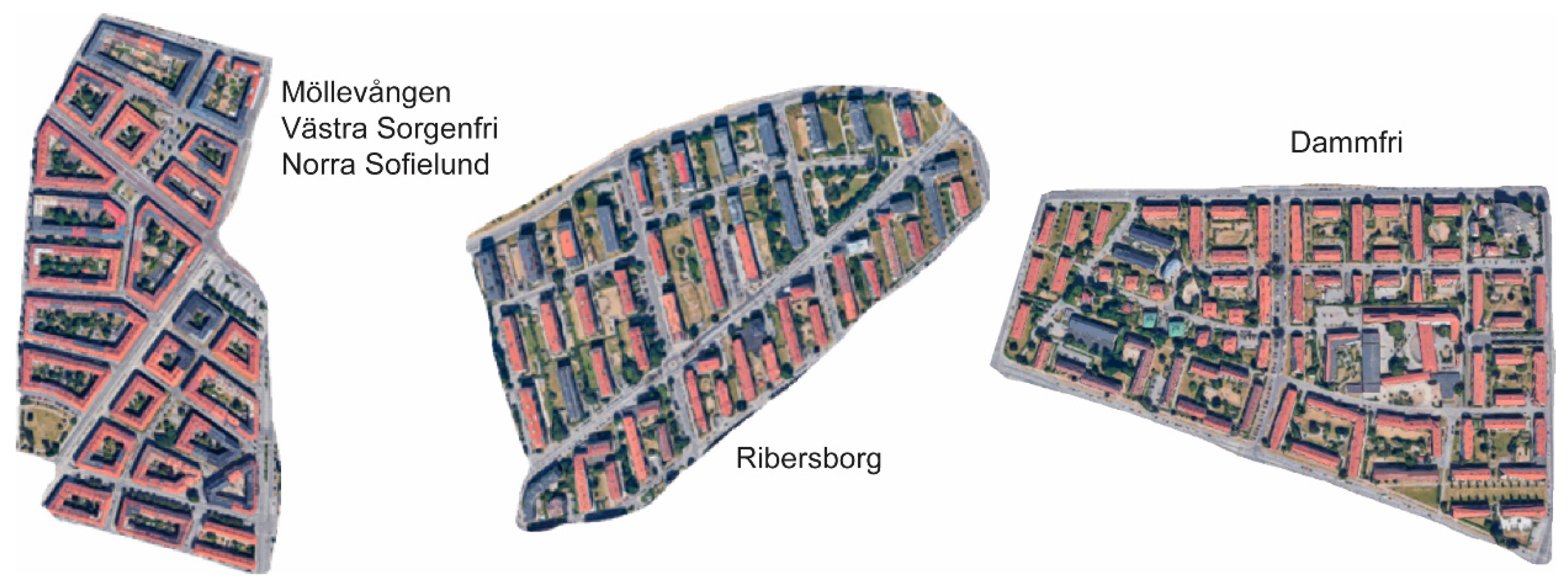
Figure 1. Examples of existing urban neighbourhoods and building types in Malmö, where slab and courtyard typologies prevail. Imagery ©2022 Google, Imagery ©2022 Lantmäteriet/Metria, Maxar Technologies, Map data ©2022.
Buildings 12 01575 g001
Figure 2. Exemplary iterations of the three studied neighbourhood typologies in top and perspective views: (A)—courtyard grid, (B)—slab grid, (C)—tower grid, and (D)—example of an analysed representative unit, comprising of one building and its plot (top view).
Buildings 12 01575 g002
Figure 3. Courtyard, slab, and tower typologies (from left to right) presented in top view at 0° rotation: The letters ‘B’ and ‘D’ denote the dimension variables specified in Table 1.
Buildings 12 01575 g003
Figure 4. Population density of the FAR metric with original mean line (blue) and removed portion of iteration cases (where FAR > 4). A box plot of the FAR dataset is included at the bottom.
Buildings 12 01575 g004
Figure 5. Map of Malmö with neighbourhood case study locations. Background map (1:50,000, raster) © Lantmäteriet (2022).
Buildings 12 01575 g005
Figure 6. Malmö neighbourhood case studies used in analysis. Case study codes link to markings in the map in Figure 5. Imagery ©2022 Google, Imagery ©2022 Lantmäteriet/Metria, Maxar Technologies, Map data ©2022.
Buildings 12 01575 g006
Figure 7. Two types of analysis surfaces (ground—left, façade—right) used to assess the outdoor and indoor environment.
Buildings 12 01575 g007
Figure 8. Two kinds of simulation point grids for façade-based metrics. Left: single string of points at 1.4 m height. Right: the whole façade made into a point grid.
Buildings 12 01575 g008
Figure 9. Correlation (Kendall) of metrics from iteration-based datasets simulated for Frankfurt and Stockholm presented in percentage format. τB values equal to 100% indicate perfect agreement. Metrics were described in Table 2.
Buildings 12 01575 g009
Figure 10. Iteration-based linear regression analysis of urban density metrics, FAR and VAR. Case studies are marked in red with labels (codes explained in Figure 5 and Figure 6).
Buildings 12 01575 g010
Figure 11. Probability distribution of VAR dataset. Blue line marks the dataset mean, and blue dots mark the case study values (codes explained in Figure 5 and Figure 6).
Buildings 12 01575 g011
Figure 12. Summary of pairwise relationships between G-metrics with graphical plots (lower half) and Pearson correlation results (upper half).
Buildings 12 01575 g012
Figure 13. Linear regression function of metrics VAR and SVF based on neighbourhood iterations (black line) and case studies (red line), including the 95% CI for the case studies regression line indicated by the grey area.
Buildings 12 01575 g013
Figure 14. Linear regression function of metrics VAR and VSC based on neighbourhood iterations (black line) and case studies (red line), including the 95% CI for the case studies regression line indicated by the grey area.
Buildings 12 01575 g014
Figure 15. Linear regression function of metrics VSC and SVF based on neighbourhood iterations (black line) and case studies (red line), including the 95% CI for the case studies regression line indicated by the grey area.
Buildings 12 01575 g015
Figure 16. Linear regression function of ground-based L-metrics RD_G and ASH_G based on neighbourhood iterations (black line) and case studies (red line), including the 95% CI for the case studies regression line indicated by the grey area.
Buildings 12 01575 g016
Figure 17. Non-linear regression functions of density metric VAR with L-metrics ASH_G (left) and RD_G (right) based on neighbourhood iterations (black line) and case-study-fitted linear regression line (red) with 95% CI in grey. The case study linear regression approximates the respective section of the non-linear regression from iterations.
Buildings 12 01575 g017
Figure 18. Linear regression function of façade-based L-metrics RD_F and ASH_F based on neighbourhood iterations (black line) and case studies (red line), including the 95% CI for the case studies regression line indicated by the grey area.
Buildings 12 01575 g018
Figure 19. Linear regression functions of metrics VAR and RD_F based on neighbourhood iterations (black line), presenting results for each neighbourhood typology in a separate graph.
Buildings 12 01575 g019
Figure 20. Non-linear regression function of density metric VAR with L-metric ASH_F based on neighbourhood iterations (black line) and case-study-fitted linear regression line (red) with 95% CI in grey.
Buildings 12 01575 g020
Figure 21. Non-linear regression function of density metric VAR and normalised EC-metric (black line) with case-study-fitted linear regression line (red) and 95% CI in grey. The graph indicates a low correlation with the scattering and clustering of data points.
Buildings 12 01575 g021
Figure 22. Linear regression function of metrics VAR and RAD_F based on neighbourhood iterations (black line) and case studies (red line), including the 95% CI for the case studies regression line indicated by the grey area.
Buildings 12 01575 g022
Figure 23. Linear regression function of façade-based metrics VSC and ASH_F based on neighbourhood iterations (black line) and case studies (red line), including the 95% CI for the case studies regression line indicated by the grey area.
Buildings 12 01575 g023
Figure 24. A suggestion for using the metric datasets in solar assessment of neighbourhood design in urban planning. In this example, the objective is daylighting of facades. Assuming target density and using the plot as an input, urban planners get suggestions for the best design options.
Buildings 12 01575 g024
Figure 25. An alternative suggestion for using the metric datasets in solar assessment of neighbourhood design in urban planning. Assuming target density, the urban planners are presented with the expected ranges of metrics as a reference to compare range values with the results of their designs.
Buildings 12 01575 g025
Figure 26. Relationship graph of metrics ASH_G and ASH_F, comparing the same metric calculated for ground and facades and presenting data points for the three analysed typologies.
Buildings 12 01575 g026
Figure 27. Selected neighbourhood cases presented as relation graphs based on the ASH on ground and façade. The graphs show cases with FAR in range of (A): (1.4–1.49), (B): (1.5–1.59), (C): (1.6–1.69), (D): (1.7–1.79).
Buildings 12 01575 g027
Table 1. Range (X-Y) and number (N, in brackets) of discrete variables used in neighbourhood design iterations and the total number of iterations.
TypologyVariablesTotal No. of Design
Iterations
[G-Metrics/Other
Metrics]
Dimension, B [m]Plot Offset [m]Building Depth, D [m]StoreysRotations [°]
Courtyard12–92 (11)8–32 (7)16 (1)2–10 (5)0–45 (2)385/770
Slab32–128 (13)8–32 (7)16 (1)2–10 (5)0–90 (3)455/1365
Tower16–20 (3)4–32 (15)=B2–20 (10)0–45 (2)450/900
Table 2. List of metrics selected for analysis. Metrics that were not sourced from literature were marked with an asterisk.
AcronymNameSubjectCalculation or Simulation Method [Unit]
G-metricsFARFloor Area RatiowholeRatio of gross floor area to plot area [m2/m2; used as unitless]
VARVolume Area RatiowholeRatio of gross building volume to plot area [m3/m2; used as unitless]
SAR *Surface Area RatiowholeRatio of gross external building surface area to plot area [m2/m2]
OSROpen Space RatiowholeRatio of open space area to gross floor area [m2/m2]
SVFSky View FactorgroundGrid-based (1 m), 145 sky patches, cosine-weighted sky dome [%]
VSCVertical Sky Componentfaçade (string)At 1.4 m height, 1024 sky patches, CIE overcast sky [%]
L-metricsAPSArea of Permanent ShadowgroundGrid-based (1 m), ray intersection, fraction of the grid open to no direct sunshine on 21 March
TH_GTwo-Hour areagroundGrid-based (1 m), ray intersection, fraction of the grid open to 2 or more hours of direct sunshine on 21 March
TH_F *Two-Hour areafaçade (string)Grid-based (1 m), ray intersection, fraction of the grid open to 2 or more hours of direct sunshine on 21 March
ASH_G *Annual Sunlight HoursgroundGrid-based (1 m), average direct solar access as fraction of all annual hourly sun vectors
ASH_F *Annual Sunlight Hoursfaçade (string)Grid-based (1 m), average direct solar access as fraction of all annual hourly sun vectors
RD_G *Reference Day (Sunlight Hours)groundGrid-based (1 m), ray intersection, average hours of direct sunshine on 21 March [h]
RD_F *Reference Day (Sunlight Hours)façade (string)Grid-based (1 m), ray intersection, average hours of direct sunshine on 21 March [h]
EC-metricsAPSHAnnual Probable Sunlight Hoursfaçade (string)Grid-based (1 m), average direct solar access as fraction of all annual hourly sun vectors (relative to cloud coverage: e.g., 40% cloudiness for a given hour gives 0.6 h of direct sun)
RAD_FSolar radiation (mean)façadeGrid-based (1 m), annual solar radiation mean per façade area [kWh/m2]
nRAD_FSolar radiation (norm.)façadeGrid-based (1 m), total annual radiation normalized by gross floor area [kWh/m2]
nPV_FPV potentialfaçadeGrid-based (1 m), surface area with solar radiation above 600 kWh/m2 normalised by floor area [m2/m2]
Table 3. The main influencing factors of each solar metric class.
G-MetricsL-MetricsEC-Metrics
geometrical dimensionsgeometrical dimensions
latitude
orientation
geometrical dimensions
latitude
orientation
insolation (climate)
Table 4. Confidence intervals (CIs) of 95% level for linear regression model coefficients of iteration- (I) and case study- (CS) based metric datasets. A metric pair is validated when CI for I data fits within the CI of CS data.
Metric PairDataInterceptSlope
Lower CIHigher CILower CIHigher CI
SVF-VARI92.492.9−5.65−5.56
CS76.3110.8−10.08−3.24
VSC-VARI38.839.0−2.65−2.61
CS33.845.8−4.25−1.87
SVF-VSCI9.8410.42.102.12
CS−13.129.01.322.96
ASH_G-VARI0.7310.740−0.061−0.059
CS0.5481.013−0.121−0.029
RD_G-VARI9.369.49−0.84−0.81
CS7.4112.6−1.54−0.52
ASH_F-VARI0.4720.476−0.032−0.032
CS0.4020.580−0.060−0.025
RD_F-VARI6.066.14−0.44−0.42
CS5.007.94−0.87−0.29
RAD_F-VARI595.3598.3−23.6−23.0
CS470.1576.2−36.8−15.8
ASH_G-RD_GI0.0580.0630.0710.071
CS−0.0170.1010.0640.086
RAD_F-VSCI252.0256.08.718.85
CS134.1237.06.4310.44
Table 5. Suggested metrics that may be suitable for early assessments of solar access at the urban planning level.
IndoorsOutdoors
DaylightingVSCSVF
SunlightingASH_FRD_G
Publisher’s Note: MDPI stays neutral with regard to jurisdictional claims in published maps and institutional affiliations.