Chinese Residents’ Willingness to Buy Housing: An Evaluation in Nanyang City, Henan Province, China Based on the Extension Cloud Model

Abstract

Real estate has always been a key industry associated with China’s economic and social development, and the real estate market has fluctuated violently in recent years. An objective and accurate evaluation of Chinese residents’ willingness to purchase housing provides a foundation for the sustainable development of the real estate industry. Accordingly, an evaluation index system and an evaluation model of Chinese residents’ willingness to buy housing were established in this study. First, the influencing factors of Chinese residents’ willingness to buy housing were systematically analyzed using Perceived Value Theory. Subsequently, the Continuous Ordered Weighted Averaging was used to assign weights to the selected index system, with smaller expert weights assigned to extreme expert opinions to reduce the subjectivity of the weight calculation results. Ultimately, an evaluation model based on the Extension Cloud Model was constructed. Residents of Nanyang City, Henan Province, China, were selected to find some distinctive conclusions. The empirical study showed that Nanyang residents were hesitant about the purchase intention of the case in April 2021, but quickly became resolute in not buying. Owing to the abrupt change in the real estate industry in China, perceived risk has become the most important risk factor. Several methods have been suggested to improve Chinese residents’ willingness to buy housing. Compared with the Analytic Hierarchy Process, the Entropy Weight Method, the fuzzy mathematics, and the grey cluster analysis, it was proved that the proposed model was more effective and advanced.

1. Introduction

In developing countries, particularly China, the real estate industry has always been the pillar industry of the national economy [1]. The stability of real estate market development plays a decisive role in national economic stability [2]. In the past 20 years, the willingness of Chinese residents to buy housing has been rising almost ceaselessly because of the continuous increase in housing cost. As a result, the annual housing sales area had increased rapidly, which had made great contributions to economic growth. However, after 2020, owing to the economic growth pressure caused by the COVID-19 epidemic [3], the drastic fluctuation of real estate policies and instances of uncompleted residential flats, the intention of Chinese consumers to buy housing involves more deliberations. In addition, their purchase intention is decreasing [4]. This has brought great obstacles to the development of China’s construction industry and economy. In the context of the drastic fluctuation of the real estate market, an accurate evaluation of the purchase intention of Chinese residents has clear guiding significance for property buyers, real estate development enterprises, and government management departments. Property buyers can judge the value of houses more rationally and manage the allocation of family assets reasonably. Real estate development enterprises can explore the key factors that affect housing transactions, and provide reference for taking targeted sales measures. For the government management department, it provides reference for the formulation of housing transaction policy.

The broad real estate market is generally divided into three levels: the market for land, the market for newly built houses, and the market for second-hand houses [5,6]. In this study, the real estate market refers to the market for newly built houses. Therefore, the willingness of residents to buy housing refers to the willingness of residents to purchase newly built commercial houses. From the perspective of maximizing perceived value, the willingness of residents to buy housing is the probability that customers purchase a commodity house, based on their existing value perception. The purchase intention discussed in this study is not for a specific commodity house but a generalized concept. With the distinct Chinese unique household registration policy, the residents in this study are Chinese urban residents, instead of farmers.

The commonly used system evaluation framework includes three parts: the evaluation index system, the determination of the index weight, and the determination of the evaluation grade [7,8].

With regard to the evaluation index system of Chinese residents’ willingness to buy housing, published studies mainly develop the evaluation index system of the purchase intention from the perspective of consumer psychology [9], economics [1], and housing value [10]. In the research field of psychology, Wu et al. [9] constructed an evaluation model of consumers’ willingness to buy housing with respect to their education level, marriage status, and future house price trends. Hentschke et al. [11] emphasized the importance of consumers’ willingness to buy in real estate development and management; further, they analyzed the main factors influencing consumers’ willingness from the perspective of real estate developers in Brazil. Wu and Zhao [10] constructed the evaluation system of apartment purchase intention of Dalian residents in China from the perspective of housing value. In addition, the current research [12,13,14] related to housing prices or residents’ purchase intention in developing countries was conducted during the period of rapid housing price increase. Since 2021, the housing environment in developing countries such as China has changed dramatically, and house prices have declined in different degrees. Therefore, the research results of those papers are probably not applicable to the current background.

For any commodity, the purchase decision of the consumer is related not only to the value of the commodity itself, but to the individual characteristics of the consumer as well. Although these studies have accomplished significant achievements, they failed to effectively identify the formation mechanism underlying the purchase intention of consumers; further, these studies impeded the comprehensive and accurate determination of the key factors affecting the purchase intention of consumers. Perceived Value Theory (PVT) divides customer attitude toward purchasing commercial housing into two parts: income belief and perceived result. It can study consumer purchase intention more comprehensively and can be successfully applied in the research field of consumer purchase intention of anti- fog cosmetics [15], energy-saving products [16], and food [17].

Owing to the complexity of the willingness of Chinese residents to buy housing, the evaluation indexes are mostly qualitative and comprehensive, and the index data are mostly obtained by expert interviews or questionnaires, which are not applicable in the objective weight calculation method or the combination weighting method containing objective weights [18]. The Analytic Hierarchy Process (AHP) is a classical subjective weight calculation method. However, the AHP is easily influenced by extreme expert opinions, rendering weight calculation results subjective [19,20]. Continuous Ordered Weighted Averaging (C-OWA) is a weighting method based on the number of combinations to improve the weighting vector. This approach assigns different expert weights to the weight information given by different experts, effectively reducing the influence of extreme expert opinions on the weight calculation results and decreasing the subjectivity of this method to a certain extent. To scientifically evaluate the risks of chemical laboratories in universities, Li et al. [20] proposed an evaluation method based on C-OWA. By empirical research, the C-OWA model was shown to fail not only in fully utilizing expert decision information but also in effectively reducing the subjectivity of weight calculation results. Kishor et al. [21] indicated that, compared with the AHP, C-OWA did not need to solve any complicated optimization problems and avoided the consistent calculation of expert opinions. Jia [22] compared decision-making methods of varying importance. The calculation and analysis of several classic examples indicated that the ranking of alternatives based on C-OWA was closer to the actual situation. Xing et al. [23] adopted C-OWA to effectively address the uncertainty of evaluation factors for the applicability of the reinforced concrete lining of high-pressure pipelines.

The commonly used system evaluation methods are Fuzzy Comprehensive Evaluation (FCE) [24] and Grey Correlation Analysis (GCA) [25]. FCE is based on function mapping and determines the evaluation grade by calculating the degree of membership between the evaluation index and the evaluation grade; however, the fuzzy uncertainty of the object to be evaluated is difficult to accurately analyze. GCA determines the evaluation grade from the grey correlation between the data of the object to be evaluated and each evaluation grade, which requires higher evaluation data. The Extension Cloud Model (ECM) introduces the cloud model into extenic and integrates the advantages of the two models [26]. Using the numerical eigenvalues of the cloud model to replace the fixed values in extension evaluation overcomes the randomness of fuzzy indexes in extension science, which easily leads to the loss of local information and realizes qualitative and quantitative conversion [27]. Aimed at the fuzzy boundary of expressway green evaluation, Hu and Cheng [28] proposed an ECM of expressway green evaluation by using the uncertainty reasoning of the cloud model and the quantification of extension theory. The result indicated that the model effectively evaluated the level of green carbon expressway. To effectively evaluate the current status of power market operation, Dong et al. [26] proposed the operation health degree of the power market and built an improved model based on the ECM. Guo et al. [29] adopted the ECM to effectively address the randomness and ambiguity in the resilience evaluation of subway construction sites. Jiang et al. [30] established an evaluation model based on the ECM to address the randomness and fuzziness of water inrush evaluation.

Therefore, PVT, C-OWA, and ECM were comprehensively used in the current study to analyze the evaluation of Chinese residents’ purchase intention. The main research contributions of this study are thus summarized. (1) The existing research results often only analyze the influencing factors from one dimension, and it is difficult to guarantee the accuracy of the follow-up evaluation. In this study, the influencing factors of Chinese residents’ purchase intention were systematically analyzed, based on PVT, from three dimensions—perceived benefits, purchase costs, and perceived risks. (2) With the use of C-OWA, the maximum and minimum values of experts’ subjective opinions were adjusted to the positions with weak influence on the weight, thus reducing the influence of experts’ extreme opinions on the weight results. (3) ECM was applied to more scientifically and effectively evaluate residents’ purchase intention. This model used the powerful uncertainty reasoning ability of the cloud model, as well as combined the capability of the matter–element extension model for comprehensive analysis. (4) Consumers in Nanyang, China, were selected to conduct the case studies, and many research conclusions with good timeliness were drawn. At present, most of the existing studies are in the rapid rise of housing prices in China or other developing countries, but this paper focused on consumers’ purchase intention under the background of drastic changes in China’s purchase environment since 2021.

2. Methodology

2.1. Evaluation Index System of Chinese Residents’ Willingness to Buy Housing

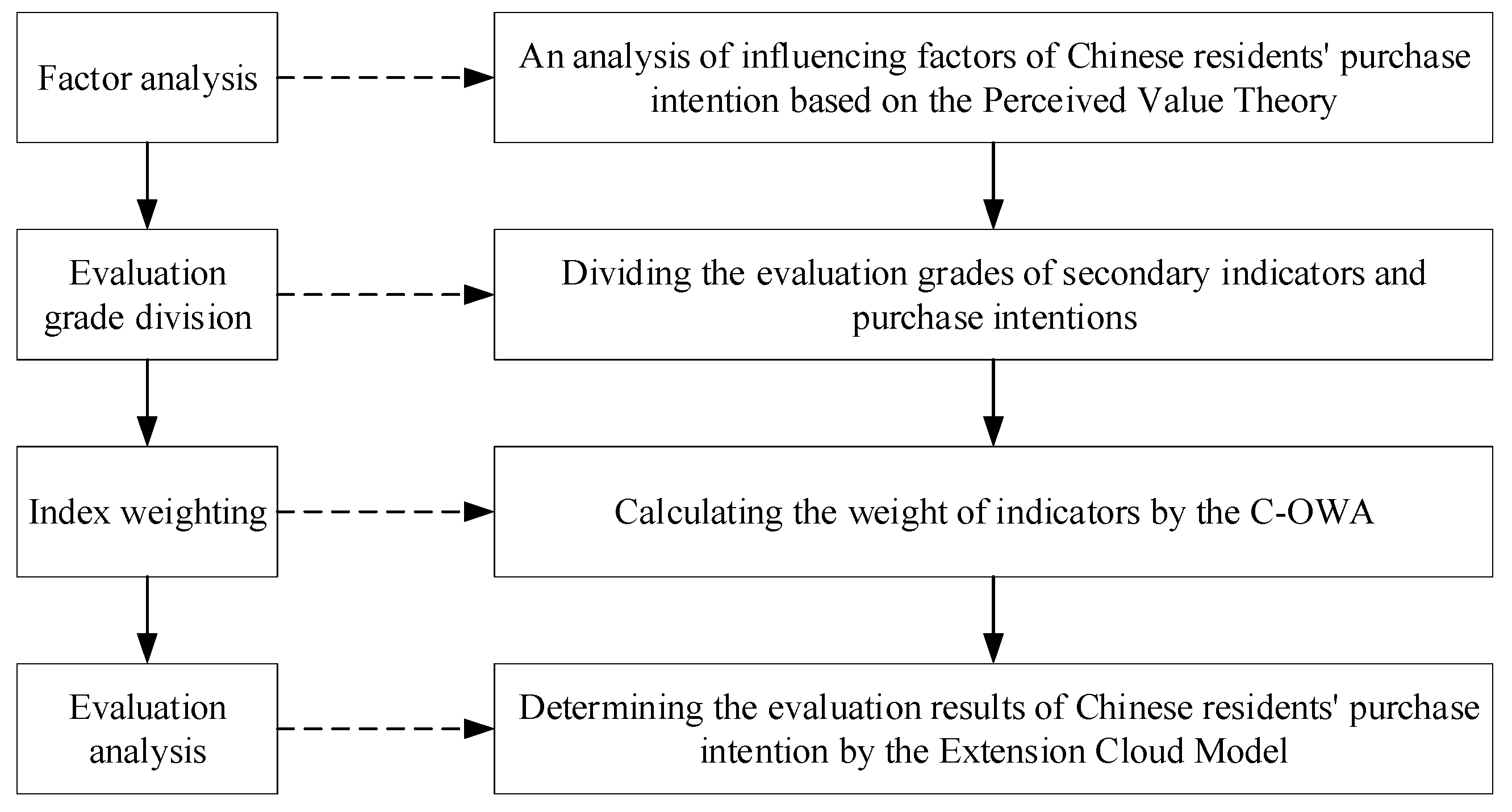
2.1.1. PVT-Based Analysis of Influencing Factors

PVT was first proposed by Zaithaml in 1988. The core concept of this theory, customer perceived value, is the overall evaluation of a product or service after the customer’s perceived profit is weighed against the cost of obtaining the product [15].

The perceived value of buyers intending to purchase real estate is also affected by perceived benefits, perceived risks, purchase costs, and other factors. The PVT-based preliminary theoretical research model of the factors influencing house purchasing is presented in Figure 1.

In Figure 1, the perceived benefits are the internal and external benefits of perceived benefits that customers feel subjectively to meet their specific consumption and psychological needs after contacting residential products and services. Purchase costs refer to the price, time, and energy paid by customers when purchasing commercial houses. Customers may not be able to directly and accurately determine the transaction price of surrounding real estate because different countries vary in real estate transaction laws. The inflation, bank rates, demand, supply, etc., are directly related to house prices. They influence the tendency of Chinese residents to buy housing by influencing house prices.

Perceived risks are the subjective judgment of customers’ perceived adverse consequences in the purchase after contacting residential products and services and feeling the on-site sales environment and atmosphere. The house is important to an ordinary family’s assets and the volatility of the national real estate policy and financial policy. Thus, customers are faced with various risks when purchasing ordinary commercial houses, such as the risk of declining prices and post-purchase anxiety. In developing countries, the perceived risk becomes one of the main factors that affect the buyers’ purchase intention as a result of the drastic fluctuation of the real estate market.

Perceived value is the customer’s measurement of their benefits, perceived costs, and risks, which is realized by contacting the products and services provided by ordinary commercial housing suppliers and assuming the purchase. Purchase intention is the probability that the customers are willing to buy an ordinary commercial house. This study maintains that consumers’ willingness is almost only related to the price–performance ratios of houses, and consumers would prioritize purchasing houses with higher price–performance ratios.

On the basis of the aforementioned analysis, the perceived benefits ($X_1$), purchase costs ($X_2$), and perceived risks ($X_3$) were selected as the primary indexes in this study. With reference to the relevant literature, secondary indexes were identified and are presented in

Table 1. Factors influencing Chinese residents’ willingness to buy housing.

Primary Index	Secondary Index	References
Perceived benefits: $X_1$	Traffic convenience: $X_{11}$	[10,11]
	Perfection of supporting facilities: $X_{12}$	[9,10,31]
	Beautiful living environment: $X_{13}$	[11,32]
	Rationality of apartment design: $X_{14}$	[4,10,31]
	Good construction quality: $X_{15}$	[9,10,33]
	Credibility of developers: $X_{16}$	[10,33]
Purchase costs: $X_2$	Affordability of house price: $X_{21}$	[12,13,14]
	Unreasonable house price: $X_{22}$	[31,33,34,35]
	Price-performance ratio: $X_{23}$	[10,36]
	Time cost: $X_{24}$	[4,37,38,39]
	Additional economic cost: $X_{25}$	[4,40]
Perceived risks: $X_3$	Price reduction: $X_{31}$	[41,42,43,44]
	Change in regional planning: $X_{32}$	[41]
	Unsatisfactory housing quality: $X_{33}$	[33,45,46]
	Possibility of being left unfinished: $X_{34}$	[2,45]
	Contract fraud: $X_{35}$	[47,48]
	Decline in loan interest rate: $X_{36}$	[49,50,51,52,53]

. Column 3 of Table 1 lists the literature sources of the secondary index.

2.1.2. Classification of Evaluation Grades

Evaluation grades are generally classified into three-grade, five-grade, and other forms [7,8]. In the current study, the five-grade evaluation, which is the most commonly used form, was selected to divide the evaluation grades of Chinese residents’ willingness to buy housing.

With reference to the classic research results of Cronin et al. [54], consumers’ purchasing intentions were classified based on three aspects: (1) the possibility of purchasing this product again, (2) the possibility of recommending it to relatives and friends, and (3) whether the same product would be chosen again given a second chance. Most residents own only one or two houses because of the high value of properties. For ordinary consumers, the possibility of buying a house again is considerably low. Thus, in this study, the possibility of purchasing this product again was replaced with whether to set this project as the first choice for house purchase. This treatment reflected the characteristics of housing transactions. The evaluation levels of the Chinese residents’ willingness to buy housing were refined. The adjusted results are shown in

Table 2. Grading of Chinese residents’ willingness to buy housing.

Grade	First Choice?	Possibility of Recommendation	Select the Same If You Choose It Again?
I	Yes	Very strong	Very firm
II	Yes	Between very intense and intense	Between very firm and firm
III	Vacillating	Strong	Firm
IV	No	Between strong and not strong	Between firmness and no regret
V	No	Not strong	With regret

.

In Table 2, I indicates that consumers have a very strong desire to purchase a house and consider the property highly valuable; II indicates that consumers have a strong desire to buy housing and consider a house valuable; III indicates that consumers are hesitant to purchase a house and consider a house as being of average value; IV indicates that consumers tend to decide against buying housing and consider it almost worthless; V indicates that consumers are unwilling to buy housing and consider it completely worthless.

2.2. Proposed Evaluation Model

2.2.1. Calculation of Weights Based on C-OWA

Ordered Weighted Averaging (OWA) was first proposed by Professor Yager in 1988 and has since then been widely used to determine the index weight [55]. This weighting method has been improved with further research. In this study, C-OWA (or OWA improved by the combination number) was used to calculate the weights assigned by experts [56]. The basic steps in C-OWA-based weight calculation for the Chinese residents’ willingness to buy housing are enumerated below.

Step 1. Collecting weight calculation data based on the Delphi method.

The residents’ representatives were invited to assign scores on evaluation indexes by importance. The scoring rules were shown in

Table 3. Index importance scoring rules.

Importance Score	Qualitative Description
1	This index is extremely important.
3	This index is very important.
5	This index is important.
7	This index is not important.
9	This index is extremely unimportant.

. If a resident representative considers a certain index crucial to purchase intention, the resident representative should rate the importance of the index as 1, 2, 4, 6, and 8, respectively, representing the degree of importance between 1 and 3, 3 and 5, 5 and 7, and 7 and 9. They were used to express the uncertainty of the residents’ representatives’ judgment regarding the importance of this index.

By collecting the score information of the index importance of the residents’ representatives, the initial importance judgment matrix $X={\left[x_{ij}\right]}_{n\times m}$ of all indexes was generated. $x_{ij}$ indicates that the $j$th resident representative rated the importance of the $i$th index. $n$ is the total number of indexes at the same level, and $m$ is the total number of residents’ representatives participating in the questionnaire survey.

Step 2. Reordering the original data.

The elements ${\left\{x_{i1},x_{i2},\cdots ,x_{ij}\right\}}^{\mathrm{T}}$ in the $i$th index importance score dataset are reordered in descending order or ascending order to generate a new sequence ${\left\{x_{i1}^{*},x_{i2}^{*},\cdots ,x_{ij}^{*}\right\}}^{\mathrm{T}}$. If the descending-order rule is adopted, the new series should meet the following rules: $x_{i1}^{*}\ge x_{i2}^{*}\ge \cdots \ge x_{ij}^{*}$. By reordering the initial importance judgment data, the extreme opinions of residents’ representatives are distributed at the beginning or the end of the series [56]. Subsequently, the sorted data point $X^{*}$ is obtained.

Step 3. Solving the weighting vector.

The influence of different residents’ representatives on the weight calculation results is referred to as the expert weight. The most common method to assign expert weights is to assign different expert weights depending on their working experience. The more experienced experts are assigned more weight, whereas the less experienced ones are assigned less weight. However, with this method, quantifying the influence of expert experience on the weight of experts presents a challenge, and the influence of extreme expert opinions on the weight calculation results cannot be eliminated. Moreover, the negative influence of extreme expert opinions on the weight calculation results is the main source of subjectivity in subjective weight calculation methods [57].

In C-OWA, the combination number $C_{n-1}^j$ is used to analyze the expert weights of resident representatives in different positions. The expert weight $d_j$ of the $j$th resident representative is expressed as follows [56]:

$$d_j=\frac{C_{n-1}^j}{{\sum }_0^{n-1}{C}_{n-1}^k}=\frac{C_{n-1}^j}{2^{n-1}}$$

(1)

The opinions of residents’ representatives at both ends (i.e., the maximum opinion or the minimum opinion) are assigned a smaller expert weight because of the calculation characteristics of the combination number.

Step 4. Determining the absolute weight of the index.

The absolute weight ${\omega }_i$ is obtained by assigning weights and summing up the sorted expert importance judgments [58]:

$${\omega }_i={\sum }_{j=1}^m{d}_j\ast x_{ij}^{*}$$

(2)

Step 5. Deriving the relative weight of each index.

By normalizing the absolute weight, the relative weight ${\omega }_i^{*}$ of the $i$th index is obtained [56]:

$${\omega }_i^{*}=\frac{{\omega }_i}{{\sum }_{i=1}^n{\omega }_i}$$

(3)

The aforementioned steps are repeated to find the relative weight vector $W=\left\{{\omega }_1^{*},\cdots ,{\omega }_n^{*}\right\}$ of all secondary indexes.

2.2.2. Evaluation Model Based on ECM

The novel evaluation model ECM combines the characteristics of matter–element theory and the cloud model [29]. The basic steps of evaluation of Chinese residents’ purchase intention based on the ECM are as follows:

Step 6. Collection of the evaluation data.

The evaluation of the purchase intention is complex and subjective. Thus, all selected secondary indexes are qualitative indexes described qualitatively. The questionnaire survey method, a typical qualitative index data processing technique, is adopted to obtain the index data [59]. The main questionnaire survey process includes the design of the questionnaire, the distribution and recovery of the questionnaire, reliability analysis, and the calculation of evaluation data.

(1)

Design of the questionnaire:

The questionnaire consisted of the following: background investigation of residents’ representatives, division of the index system and evaluation grade, and collection of index data.

(2)

Distribution and recovery of questionnaires:

Questionnaires are generally distributed in two ways: on-the-spot investigation and online investigation [60]. The first method has the advantages of a wide range of influence and involvement of numerous experts but has the disadvantage of low efficiency of the investigation results. The second method has the advantage of high survey results; however, the approach entails a heavy workload, and the number of questionnaires collected is small. Among the data in this study are a large number of residents’ representatives. With this factor considered, the online investigation allows the distribution and collection of the questionnaire.

(3)

Reliability analysis of questionnaire survey results

After the invalid questionnaires are eliminated, their reliability needs to be analyzed. Cronbach’s α coefficients are calculated by importing the questionnaire results into the SPSS 19.0 software. Generally speaking, the Cronbach’s α coefficients greater than 0.7 generally indicates good reliability [61].

(4)

Calculation of the evaluation data:

The quantitative scoring of each secondary index by residents is the score of this index.

Step 7. Determining the evaluation standard cloud.

Before the evaluation standard cloud is calculated, the calculation of the cloud model parameters $\left(Ex,En,He\right)$ is briefly introduced.

$Ex$ is the expectation of the cloud, indicating the mathematical expectation of all cloud droplets in the universe and reflecting the position of the center of gravity of the cloud. $En$ is the entropy of cloud, which is reflected in the acceptable range of linguistic values in the universe of discourse—that is, the ambiguity and the probability of corresponding linguistic values. $He$. is the super entropy, which is the entropy of $En$. It reflects the cohesion of the uncertainty of all linguistic value points in the universe of discourse.

To facilitate the subsequent quantitative research, the qualitative description of the evaluation grade in Table 2 is converted into a quantitative description. The five evaluation grades, together with their corresponding scores, are Ⅰ [0, 25], II (25, 50], III (50, 75], Ⅳ (75, 90], and V (90, 100].

The standard cloud of Chinese residents’ willingness to buy housing is given below [26]:

$$R^{*}=\left(N,C_k,v_k^{*}\right)=\left[\begin{array}{ccc}N& C_1& \left(E{x}_1^{*},E{n}_1^{*},H{e}_1^{*}\right)\\ & C_2& \left(E{x}_2^{*},E{n}_2^{*},H{e}_2^{*}\right)\\ & C_3& \left(E{x}_3^{*},E{n}_3^{*},H{e}_3^{*}\right)\\ & C_4& \left(E{x}_4^{*},E{n}_4^{*},H{e}_4^{*}\right)\\ & C_5& \left(E{x}_5^{*},E{n}_5^{*},H{e}_5^{*}\right)\end{array}\right]$$

(4)

where $k=1,2,\cdots ,5$ represents five evaluation levels, and $v_k^{*}$ represents the parameters of the standard cloud of the $k$th evaluation level.

The calculation methods for $E{x}_k^{*}$, $E{n}_k^{*}$, and $H{e}_k^{*}$ in Equation (4) are given below [26,28]:

$$E{x}_k^{*}=\frac{a_k+b_k}{2}$$

(5)

$$E{n}_k^{*}=\frac{b_k-a_k}{6},$$

(6)

$$H{e}_k^{*}=s,$$

(7)

where $a_k$ and $b_k$ are the upper and lower limits of the value interval corresponding to the $k$th evaluation grade. In addition, $s$ is a constant, the value of which is adjusted and determined by the manager, depending on the actual situation of the evaluation object and the evaluation result.

Step 8. Determining the matter element to be evaluated.

According to the principle of the ECM, the matter elements to be evaluated for each secondary index are given below [26]:

$$R=\left[\begin{array}{ccc}N& C_1& v_1\\ & C_2& v_2\\ & ⋮& ⋮\\ & C_n& v_n\end{array}\right]=\left[\begin{array}{ccc}N& C_1& \left(E{x}_1,E{n}_1,H{e}_1\right)\\ & C_2& \left(E{x}_2,E{n}_2,H{e}_2\right)\\ & ⋮& ⋮\\ & C_n& \left(E{x}_n,E{n}_n,H{e}_n\right)\end{array}\right]=\left[\begin{array}{c}{R}_1\\ R_2\\ \begin{array}{c}⋮\\ R_n\end{array}\end{array}\right].$$

(8)

The key to determining the matter element to be evaluated is to calculate the cloud parameters $\left(E{x}_i,E{n}_i,H{e}_i\right)$ of the $i$th secondary index of the research object.

The calculation methods for $E{x}_i$, $E{n}_i$, and $H{e}_i$ are as follows [26,28]:

$$E{x}_i=\frac{1}{m}{\sum }_{j=1}^m{x}_{ij},$$

(9)

$$E{n}_i=\sqrt{\frac{\pi }{2m^2}}{\sum }_{j=1}^m{\left(x_{ij}-E{x}_i\right)}^2$$

(10)

$$H{e}_i=\sqrt{\left|\frac{1}{m-1}{\sum }_{j=1}^m{\left(x_{ij}-E{x}_i\right)}^2-{\left(E{n}_i\right)}^2\right|},$$

(11)

where $x_{ij}$ represents the score of the $j$th resident representative on the $i$th index.

By substituting the data obtained in Step 6 into Equations (9)–(11), the matter elements of each secondary index to be evaluated are derived obtained.

Step 9. Calculating the degree of correlation.

In the cloud model, each secondary index in the evaluation of Chinese residents’ purchase intention was regarded as a cloud drop. In this study, the forward cloud generator was selected to calculate the correlation evaluation degree. The forward cloud generator obtains the quantitative value of the output cloud droplets through three numerical characteristics of the input cloud model. The algorithm of the forward cloud generator is as follows:

Input: three numerical eigenvalues $\left\{\left.Ex,En,He\right\}\right.$ representing qualitative concept clouds and $N$ of cloud droplets to be generated.

Output: the quantitative values of $N$ cloud droplets and the certainty of each cloud droplet.

(1)

Generating a normal random number $E{x}_p=Norm\left(En,H{e}^2\right)$;

(2)

Generating a normal random number $x_p=Norm\left(Ex,E{x}_p^2\right)$;

(3)

The calculation method for the cloud correlation degree ${\mu }_{ki}$ between the $i$th index and the $k$th level boundary cloud model is given below [26,28]:

$${\mu }_{ki}=e^{-\frac{{\left(x_p-Ex\right)}^2}{2E{n}_i^2}}.$$

(12)

Step 10. Determining the risk level.

By determining the weighted correlation coefficient, the comprehensive evaluation vector $D=\left\{d_1,d_2,d_3,d_4,d_5\right\}$ is derived. The calculation equation for $d_k$ is as follows [26]:

$$d_k={\sum }_{i=1}^n{\omega }_i^{*}\ast {\mu }_{ki}.$$

(13)

The weighted average method is used to obtain the fuzzy grade eigenvalue [26]:

$$r=\frac{{\sum }_{i=1}^5{d}_i{f}_i}{{\sum }_{i=1}^5{d}_i},$$

(14)

where $f_i$ represents the score corresponding to the $i$th evaluation level. $f_i$ is expressed as a positive integer from 1 to 5, representing the risk evaluation grades from grade I to grade V, respectively.

The normal random number is generated with strong randomness, resulting in errors and inaccuracies in the calculation results. Therefore, it has to be solved several times to minimize the uncertainty caused by random factors. Through 1000 calculations, the expected value $E_r$ of $r$ is determined [26]:

$$E_r=\frac{{\sum }_{a=1}^{1000}{r}_a}{1000},$$

(15)

where $r_a$ is the comprehensive evaluation index value calculated using the $a$th operation.

The final evaluation grade can be obtained by comparing $E_r$ with the evaluation grade. The relationship between the evaluation grades and the expected value $E_r$ is listed in

Table 4. Evaluation Grade.

Evaluation Grade	I	II	III	IV	V
$E_r$	[0, 1.5)	[1.5, 2.5)	[2.5, 3.5)	[3.5, 4.5)	[4.5, +∞)

.

Step 11. Verifying the evaluation results.

$E_r$ is an important index for measuring the dispersion degree of evaluation results, and its size is directly proportional to the degree of dispersion of the evaluation results [26]. $E_{rn}$ is calculated as follows:

$$E_{rn}=\sqrt{\frac{1}{1000}{\sum }_{a=1}^{1000}{\left[r_a-E_r\right]}^2}.$$

(16)

In verifying the objectivity and credibility of the evaluation results, the credibility factor $\theta$ is introduced to test the evaluation results. $\theta$ is calculated as follows:

$$\theta =\frac{E_{rn}}{E_r}.$$

(17)

The greater the $\theta$, the higher the dispersion of the evaluation results and the lower the objective credibility; the smaller the $\theta$, the lower the dispersion of the evaluation results and the higher the degree of objective credibility. $\theta <0.01$ generally indicates that the evaluation result is objective and credible [26].

2.3. Flowchart of the Proposed Model

To facilitate readers to understand and use the proposed method, the research framework and the flow chart were shown in Figure 2 and Figure 3, respectively.

3. Case Study

3.1. Study Area and Data Sources

The study area selected in this paper is Nanyang City, Henan Province, China. Nanyang is a sub-central city, and it has a total area of 26,509 km² and a resident population of 9,713,112. In 2021, Nanyang achieved a regional GDP of 434.222 billion CNY, with a per capita GDP of 38,064 CNY. The per capita housing area of urban residents in Nanyang was about 36 m², which was lower than the national average. The average price of newly built commercial houses in Nanyang was 8302 CNY/m².

Nanyang is a typical medium-sized city in China, and its economic and social development is very representative. Nanyang’s real estate market is also very representative. In recent years, typical real estate events in China, such as the development of high-speed rail, the reform of school districts, the phenomenon of unfinished buildings, and the destocking of commercial houses, have almost happened here. The authors of this manuscript have studied Nanyang real estate market for a long time and collected a large amount of information. This provides the basis for the research of this paper. Jianye Dacheng Courtyard Project is a new real estate development project in Nanyang in recent years. Therefore, the residents’ willingness to buy housing for Jianye Dacheng Courtyard Project in Nanyang was selected as a case study.

The house cost of Jianye Dacheng Courtyard Project is 8500 CNY/m², slightly higher than the average house price in Nanyang. Developed by Nanyang Magnolia Real Estate Co., Ltd., it is located on the south side of the intersection of Xuefeng Road and Zhongjing South Road in Wancheng District. The project was sold on 1 April 2021 and is expected to be delivered on 30 December 2023. Specific information on this project can be found on the website (https://ny.fang.anjuke.com/loupan/canshu-466334.html?from=loupan_tab, accessed on 1 April 2021).

The research data of this paper mainly included weight calculation data and all secondary index scores. The questionnaire survey was used to obtain these data. The questionnaires prepared in this study were distributed through an online platform and filled out by all respondents from 1 April to 30 April 2021. A total of 129 questionnaires were collected, including 37 invalid questionnaires and 92 valid questionnaires. The valid questionnaires had a recovery rate of 71.32%.

This questionnaire was divided into three parts: (1) Personal basic information of residents’ representatives, which included sex, age, marital status, education level, occupation, monthly income level, city, and existing housing situation, among others. (2) Collection of index weight information. Residents’ representatives were invited to assign scores on indexes by importance in accordance with the scoring rules in Table 3. (3) Collection of evaluation data. Residents’ representatives were invited to assign scores on the indexes in accordance with the scoring rules in Section 4.2.

The collected data from 92 valid questionnaires were brought into SPSS 19.0 software, and the Cronbach’s α coefficients of the weight data and score data were calculated. The results are listed in

Table A1. Cronbachs’α coefficients of valid questionnaires.

Secondary Indexes	Weight Calculation Information	Index Score
$X_{11}$	0.7876	0.7490
$X_{12}$	0.7354	0.7422
$X_{13}$	0.7227	0.7648
$X_{14}$	0.8533	0.8090
$X_{15}$	0.7021	0.7422
$X_{16}$	0.7838	0.8648
$X_{21}$	0.7872	0.7574
$X_{22}$	0.8142	0.8231
$X_{23}$	0.8881	0.7688
$X_{24}$	0.7319	0.8711
$X_{25}$	0.7282	0.7273
$X_{31}$	0.7269	0.7949
$X_{32}$	0.8312	0.9057
$X_{33}$	0.7384	0.7426
$X_{34}$	0.7605	0.8712
$X_{35}$	0.8279	0.7760
$X_{36}$	0.8015	0.8331

.

All Cronbach’s α coefficients in Table A1 exceed 0.7, which proves the good reliability of this questionnaire survey results [61]. The scores of the secondary indexes are presented in

Table A2. Scores of secondary indexes.

Index	(1)	(2)	(3)	(4)	(5)	$\cdots$	(87)	(89)	(90)	(91)	(92)	Average Score
$X_{11}$	30	35	20	25	40	$\cdots$	45	35	25	20	20	27.5442
$X_{12}$	20	15	25	35	20	$\cdots$	15	35	30	25	20	22.8496
$X_{13}$	45	50	45	40	55	$\cdots$	60	65	75	70	55	58.7422
$X_{14}$	25	35	40	25	20	$\cdots$	30	45	50	20	25	30.4081
$X_{15}$	45	25	15	10	10	$\cdots$	15	10	15	5	25	18.2530
$X_{16}$	50	70	60	65	55	$\cdots$	65	75	60	75	60	66.5728
$X_{21}$	25	35	40	30	20	$\cdots$	40	45	35	50	50	40.2721
$X_{22}$	60	55	65	70	45	$\cdots$	45	50	60	65	45	61.4391
$X_{23}$	90	85	95	90	90	$\cdots$	95	95	95	80	90	92.4368
$X_{24}$	25	30	30	35	40	$\cdots$	35	30	25	15	20	30.4081
$X_{25}$	60	50	45	50	55	$\cdots$	75	60	60	50	45	63.4224
$X_{31}$	40	35	50	45	45	$\cdots$	30	45	35	45	40	37.5465
$X_{32}$	75	70	60	65	50	$\cdots$	70	60	65	75	80	73.6444
$X_{33}$	70	75	80	85	60	$\cdots$	60	55	50	60	75	68.6181
$X_{34}$	45	50	75	40	60	$\cdots$	70	45	60	55	65	61.4344
$X_{35}$	35	30	25	40	40	$\cdots$	35	45	50	55	40	42.5823
$X_{36}$	55	65	60	45	60	$\cdots$	60	45	65	55	45	61.4344

. Only some expert scoring data are listed in Table A2 because of space limitations.

3.2. Calculation of Index Weight

By substituting the acquired index importance information into Equations (1)–(3), all secondary index weights were derived. The results are listed in

Table A3. Calculation results for index weights by the C-OWA.

Index	Local Weight		Comprehensive Weight
	Weight	Ranking	Weight	Ranking
$X_1$	0.336	2	-	-
$X_2$	0.361	1	-	-
$X_3$	0.302	3	-	-
$X_{11}$	0.097	4	0.033	10
$X_{12}$	0.161	3	0.054	8
$X_{13}$	0.269	2	0.090	6
$X_{14}$	0.091	5	0.030	12
$X_{15}$	0.070	6	0.024	15
$X_{16}$	0.312	1	0.105	3
$X_{21}$	0.078	5	0.028	14
$X_{22}$	0.262	2	0.095	4
$X_{23}$	0.257	3	0.093	5
$X_{24}$	0.090	4	0.033	11
$X_{25}$	0.313	1	0.113	2
$X_{31}$	0.067	5	0.020	16
$X_{32}$	0.454	1	0.137	1
$X_{33}$	0.099	4	0.030	13
$X_{34}$	0.202	2	0.061	7
$X_{35}$	0.008	6	0.002	17
$X_{36}$	0.170	3	0.051	9

.

Owing to space limitations, only three primary indexes are used as examples to reveal the calculation details based on C-OWA.

Step 1. Determining the index weight by using the Delphi method.

A total of 92 experts rated the three secondary indicators by importance. The initial decision data $X={\left[x_{ij}\right]}_{3\times 92}$ of the importance of the three indicators were determined. Some initial decision data are presented in

Table A4. Importance scores of three primary indexes.

Resident	(1)	(2)	(3)	(4)	(5)	(6)	(7)	(8)	(9)	(10)
$X_1$	6.5	5	7	4.5	5	6.5	6	7.5	5.5	6
$X_2$	4.5	7.5	4.5	5	4.5	5	4.5	5	4.5	6.5
$X_3$	5.5	6.5	6	5.5	5	5.5	6	4.5	7.5	5
Resident	(11)	(12)	(13)	(14)	(15)	$\mathbf{\cdots }$	(79)	(80)	(81)	(82)
$X_1$	7	5	5.5	6.5	6	$\cdots$	4.5	5	7.5	6.5
$X_2$	6	6.5	6	5	4.5	$\cdots$	7	6.5	4.5	6
$X_3$	5.5	5.5	4.5	4.5	6.5	$\cdots$	5	5.5	8	7
Resident	(83)	(84)	(85)	(86)	(87)	(88)	(89)	(90)	(91)	(92)
$X_1$	8	6.5	7.5	6	4.5	8	6.5	7.5	7	7.5
$X_2$	6	4.5	5	6.5	6	4.5	5	6.5	7.5	5
$X_3$	6.5	5	6.5	5.5	4.5	5	6.5	4.5	7	7.5

.

Step 2. Reordering the initial expert importance judgment data $X$ to obtain the sorted data $X^{*}$.

Subsequently, the elements ${\left\{x_1,x_2,\cdots ,x_j\right\}}^{\mathrm{T}}$ in the six second-level index importance score datasets were reordered in descending order. The sorted results are shown in Columns 4–6, 8–10, and 13–15 of

Table A5. Weight calculation of primary indexes.

Re-Order	1	2	3	4	5	6	7	8	$\mathbf{\cdots }$
$d_j$	0.000	0.000	0.000	0.000	0.000	0.000	0.000	0.000	$\cdots$
$X_1$	8.5	8.5	8	8	8	8	8	8	$\cdots$
$X_2$	9	9	9	9	9	9	8.5	8.5	$\cdots$
$X_3$	8	8	8	8	8	8	8	8	$\cdots$
Re-order	42	43	44	45	46	47	48	49	50
$d$	0.054	0.064	0.073	0.079	0.083	0.083	0.079	0.073	0.064
$X_1$	6	6	6	6	6	6	6	5.5	5.5
$X_2$	6.5	6.5	6.5	6	6	6	6	6	6
$X_3$	5.5	5.5	5.5	5.5	5.5	5.5	5.5	5.5	5.5
Re-order	$\mathbf{\cdots }$	85	86	87	88	89	90	91	92
$d$	$\cdots$	0.000	0.000	0.000	0.000	0.000	0.000	0.000	0.000
$X_1$	$\cdots$	4	3.5	3.5	3.5	3.5	3.5	3.5	3.5
$X_2$	$\cdots$	4	4	4	3.5	3.5	3.5	3.5	3.5
$X_3$	$\cdots$	3	3	3	3	3	3	3	3

.

Step 3. Calculating the expert weight to solve the weight vector $d_j$.

The number of resident representatives participating in the evaluation was 92. In accordance with Equation (1), the weighted vector of the residents’ representatives in each secondary index was determined, and the calculation results are shown in Columns 2, 7, and 12 in Table A5.

Step 4. Using Equation (2) to assign weights and sum up the ranked expert importance judgments to determine the absolute weight ${\omega }_i$ of each index, as shown in

Table 5. Weight calculation results for the three primary indexes.

Primary Index	${\mathit{X}}_{\mathbf{1}}$	${\mathit{X}}_{\mathbf{2}}$	${\mathit{X}}_{\mathbf{3}}$
Absolute weight	4.487	4.822	4.034
Final weight	0.336	0.361	0.302

.

Step 5. Normalizing the absolute weights of the three primary indexes by using Equation (3) to determine the relative weight of each index, as shown in Table 5. By performing similar steps, the relative weights and absolute weights of all secondary indexes can be derived.

3.3. Determination of the Evaluation Grade

Step 6. Collection and analysis of data. Section 2.1 presents the evaluation data collected and analyzes the reliability of the evaluation data.

Step 7. Calculation of the standard cloud. The expectation and entropy of the evaluation standard cloud were determined by substituting the upper and lower limits of the five evaluation grade intervals into Equations (5) and (6). The super entropy was set as 0.002 [26]. Thus, the standard cloud is as follows:

$$R^{*}=\left(N,C_k,v_k^{*}\right)=\left[\begin{array}{ccc}N& C_1& \left(12.5,12.5,0.002\right)\\ & C_2& \left(37.5,12.5,0.002\right)\\ & C_3& \left(62.5,12.5,0.002\right)\\ & C_4& \left(82.5,7.5,0.002\right)\\ & C_5& \left(95,5,0.002\right)\end{array}\right].$$

(18)

Step 8. Determining the matter element to be evaluated.

The scores of each secondary index were substituted into Equations (9)–(11), and the object elements of each secondary index were determined. The results are listed in

Table A6. Cloud model parameters of secondary indexes.

Index	$\mathit{E}{\mathit{x}}_{\mathit{i}}$	$\mathit{E}{\mathit{n}}_{\mathit{i}}$	$\mathit{H}{\mathit{e}}_{\mathit{i}}$	Index	$\mathit{E}{\mathit{x}}_{\mathit{i}}$	$\mathit{E}{\mathit{n}}_{\mathit{i}}$	$\mathit{H}{\mathit{e}}_{\mathit{i}}$
$X_{11}$	27.5442	9.547	0.105	$X_{24}$	30.4081	6.763	0.088
$X_{12}$	22.8496	6.316	0.085	$X_{25}$	63.4224	18.315	0.145
$X_{13}$	58.7422	15.878	0.135	$X_{31}$	37.5465	5.764	0.081
$X_{14}$	30.4081	12.731	0.121	$X_{32}$	73.6444	14.451	0.129
$X_{15}$	18.2530	15.288	0.132	$X_{33}$	68.6181	15.514	0.133
$X_{16}$	66.5728	8.746	0.100	$X_{34}$	61.4344	18.147	0.144
$X_{21}$	40.2721	12.764	0.121	$X_{35}$	42.5823	10.260	0.108
$X_{22}$	61.4391	13.627	0.125	$X_{36}$	61.4344	11.605	0.115
$X_{23}$	92.4368	3.263	0.061	-	-	-	-

.

Step 9. Determining the cloud correlation degree.

The calculation results in Table A6 were input into the forward cloud generator to calculate the cloud correlation degree, (Table A6). Bold type indicates weighted cloud correlation degrees, whereas normal font indicates unweighted in Table A6.

Step 10. Determining the risk level.

By assigning a weight to the correlation coefficient in Table A6 in accordance with Equation (13), the comprehensive evaluation vector $D$ was derived (

Table A7. Cloud correlation degree of secondary indicators.

Index	Ⅰ		II		III		Ⅳ		V
$X_{11}$	0.847	0.028	0.136	0.004	0.017	0.001	0	0	0	0
$X_{12}$	0.988	0.053	0.012	0.001	0	0	0	0	0	0
$X_{13}$	0.002	0	0.250	0.023	0.748	0.067	0	0	0	0
$X_{14}$	0.163	0.005	0.837	0.025	0	0	0	0	0	0
$X_{15}$	0.996	0.024	0.004	0	0	0	0	0	0	0
$X_{16}$	0	0	0.014	0.001	0.832	0.087	0.154	0.016	0	0
$X_{21}$	0	0	0.797	0.022	0.203	0.006	0	0.000	0	0
$X_{22}$	0	0	0.101	0.010	0.845	0.080	0.054	0.005	0	0
$X_{23}$	0	0	0	0	0	0	0.046	0.004	0.954	0.089
$X_{24}$	0.001	0	0.841	0.028	0.058	0.002	0	0	0	0
$X_{25}$	0	0	0	0	0.842	0.095	0.158	0.018	0	0
$X_{31}$	0.109	0.002	0.764	0.015	0.127	0.003	0	0	0	0
$X_{32}$	0	0	0.	0	0.719	0.099	0.261	0.036	0.020	0.003
$X_{33}$	0	0	0.119	0.004	0.739	0.022	0.142	0.004	0	0
$X_{34}$	0	0	0.175	0.011	0.682	0.042	0.143	0.009	0	0
$X_{35}$	0.160	0	0.804	0.002	0.036	0.000	0	0	0	0
$X_{36}$	0	0	0.153	0.008	0.815	0.042	0.042	0.002	0	0

). By inputting $D$ into Equation (14), the fuzzy grade characteristic value of 2.887 is thus determined. Exactly 1000 repeated calculations were performed to minimize the effect of uncertainty due to random factors. The expected value $E_r$ was 2.8974. As shown in Table 4, the evaluation grade of the case is III.

Step 11. Verifying evaluation results.

The result of the repeated calculation was substituted into Equation (16), and $E_{rn}$ was calculated as 0.0254. In accordance with Equation (17), the credibility factor was calculated as 0.0088, which is less than 0.01. The evaluation result was determined to be objective and credible.

In summary, the purchase intention of the case was III, and this result exhibited high credibility. This study proposes some countermeasures and suggestions for marketing Jianyang Dacheng Courtyard Project in Nanyang to enhance residents’ willingness to purchase houses for the case project.

(1)

Creation of the selling point of the project location.

As determined from the case study, consumers in Nanyang are sensitive to the location and surrounding plan for the project. The location and surrounding plan are among the concerns of buyers. Their rationality directly affects the transportation convenience of buyers, and the surrounding supporting facilities directly influence the quality of life and the appreciation space of real estate. Therefore, when selecting the site for development, the developer should pay attention to the traffic status and future development of the plot. In addition, during development and construction, the developer should consciously create the surrounding safe environment, shopping environment, greening environment, educational environment, and sanitary environment, among others. Such environments include public security spots, large supermarkets, shopping malls, restaurants, schools, banks, hospitals, playgrounds, parks, and stadiums.

(2)

Reasonable pricing and reduction in extra costs for consumers to buy housing.

In the case study, the purchase cost was identified as the most important reason hindering buyer purchase. Consumers often want to spend the least money to acquire the most desirable commercial housing. When consumers perceive that the price is unreasonable or the price may decrease, they will not buy it to a large extent. In addition, the extra cost of buying housing will also significantly hurt consumer confidence in buying housing. Therefore, real estate sales enterprises should adopt a reasonable pricing strategy, exude sincerity, and let consumers feel the greatest value. On the one hand, enterprises can adopt a diversified marketing mix to promote sales according to the actual situation in order to attract consumers and make them feel valued. On the other hand, depending on the actual situation, some enterprises may consider signing an insurance agreement with the buyers within a certain period to increase confidence in the buyers. In addition, due to the popularity of COVID-19, house prices have been re-evaluated by most consumers [62,63]. Developers should fully evaluate its impact and adopt more flexible pricing strategies.

(3)

Strict implementation of the supervision system of pre-sale funds to enhance the reputation of developers.

Since 2021, many real estate development enterprises in China have successively defaulted and delayed the delivery of commercial houses. This occurrence has negatively affected the confidence of Chinese buyers. China’s commercial housing still adopts the pre-sale system, hence the inevitability of avoiding the supervision of pre-sale funds. Developers should strictly implement the supervision system of pre-sale funds in Nanyang. In this system, the developer shall deposit the entire amount paid by the purchaser into the pre-sale fund supervision account, including the deposit, down payment, installment payment, one-time payment, bank mortgage loan, housing accumulation fund loan, and the full decoration of commercial housing, among others, and shall not use the non-presale fund supervision account to deposit the amount paid by the purchaser. Sales funds are first allocated to project construction to ensure the completion and delivery of real estate projects. In addition, the developer can actively publicize it through the consumers who have purchased it in the early stage. Trust between buyers is higher than that between buyers and developers.

4. Discussion

4.1. Effect of Different Evaluation Index Systems on the Evaluation Results

The rationality of the index system significantly affects the evaluation results. The final evaluation result is obtained by combining the evaluation results of all secondary indexes. Different evaluation index systems not only mean that the influencing factors of residents’ purchase intention are different, but also have a significant impact on the final evaluation results. The more secondary indicators, the greater the research workload, and the more accurate the evaluation results are. Finding the smallest index set for a case via the commonly used trial-and-error algorithm presents a challenge. Therefore, in this study, rough set (RS) theory was used to identify the unnecessary secondary indicators listed in Table 1 and thereby reduce the amount of calculation. The operating method of the Rosetta system is found in [64].

After rough set processing, $X_{14}$, $X_{15}$, $X_{21}$, and $X_{31}$ were regarded as unnecessary secondary indexes. Unnecessary secondary indicators were thus deleted. The evaluation results of the case are shown in

Table 6. Influence of different evaluation index systems on evaluation results.

Deleted Indexes	${\mathit{E}}_{\mathit{r}}$	Evaluation Results	Deleted Indexes	${\mathit{E}}_{\mathit{r}}$	Evaluation Results
None	2.8974	III	$X_{15}$, $X_{21}$	2.8532	III
$X_{14}$	2.9862	III	$X_{15}$, $X_{31}$	2.9515	III
$X_{15}$	2.8417	III	$X_{21}$, $X_{31}$	3.2714	III
$X_{21}$	2.7944	III	$X_{14}$, $X_{15}$, $X_{21}$	2.9589	III
$X_{31}$	2.9930	III	$X_{14}$, $X_{15}$, $X_{31}$	2.8317	III
$X_{14}$, $X_{15}$	3.0314	III	$X_{14}$, $X_{21}$, $X_{31}$	2.8400	III
$X_{14}$, $X_{21}$	2.8843	III	$X_{15}$, $X_{21}$, $X_{31}$	2.4574	II
$X_{14}$, $X_{31}$	3.0199	III	$X_{14}$, $X_{15}$, $X_{21}$, $X_{31}$	2.3460	II

.

As shown in Table 6, deleting $X_{15}$, $X_{21}$, $X_{31}$ or deleting $X_{14}$, $X_{15}$, $X_{21}$, $X_{31}$ significantly affected the evaluation results. Therefore, this study had three minimum sets of indicators: (1) deleting $X_{14}$, $X_{15}$, and $X_{21}$; (2) deleting $X_{14}$, $X_{15}$, and $X_{31}$; and (3) deleting $X_{14}$, $X_{21}$, and $X_{31}$. The other 14 secondary indicators were retained. Obviously, the workload of using 14 secondary indicators for evaluation is far less than the original 17 secondary indicators.

Notably, different cases or different evaluation index systems could lead to different minimum index sets. For other projects, the idea of Section 4.1 can be used to find the smallest set with pertinence.

4.2. Dynamic Analysis of Residents’ Purchase Intention

It takes a long time for consumers to purchase commercial housing from the purchase intention to the final completion of the purchase. Thus, this section demonstrates our attempt to analyze the purchase intention of residents in Nanyang, China at different time points, to realize the dynamic evaluation.

A review of the development history of China’s real estate market in 2021 reveals that this study repeated the research on the evaluation of purchase intention in the following three periods. (1) 1 July 2021–31 July 2021. Evergrande Group, once the largest real estate developer in China, officially announced its breach of contract in June 2021, delaying the delivery of the developed real estate. Such an event exerts a significant negative effect on residents’ purchase intentions. (2) 1 January 2022–31 January 2022. In December 2021, the Chinese government began to intensively introduce stimulus policies for the real estate industry. January is also the peak season for commercial housing sales in China, as observed in the past 20 years. This event has a significant positive effect on residents’ purchase intention. (3) 1 June 2022–30 June 2022. On 16 May 2022, the People’s Bank of China announced that the interest rate of the first home loan would be reduced by 20 BP. This event has a significant positive influence on residents’ purchase intention. The residents who participated in the first round of questionnaires were selected for the three questionnaires that followed.

The weight calculation results for the residents’ purchase intention indicators in four different periods are presented in

Table A8. Calculation of index weights at different time points.

Index	April 2021		July 2021		January 2022		June 2022
	Weight	Ranking	Weight	Ranking	Weight	Ranking	Weight	Ranking
$X_1$	0.336	2	0.296	2	0.220	3	0.269	2
$X_2$	0.361	1	0.274	3	0.268	2	0.240	3
$X_3$	0.302	3	0.430	1	0.510	1	0.490	1
$X_{11}$	0.033	10	0.039	14	0.028	16	0.027	14
$X_{12}$	0.054	8	0.077	5	0.040	13	0.066	8
$X_{13}$	0.090	6	0.054	9	0.032	15	0.054	11
$X_{14}$	0.030	12	0.010	17	0.040	10	0.027	15
$X_{15}$	0.024	15	0.048	10	0.040	11	0.074	7
$X_{16}$	0.105	3	0.068	6	0.040	12	0.021	17
$X_{21}$	0.028	14	0.047	11	0.072	6	0.024	16
$X_{22}$	0.095	4	0.031	15	0.071	7	0.052	12
$X_{23}$	0.093	5	0.068	7	0.027	17	0.056	10
$X_{24}$	0.033	11	0.045	12	0.036	14	0.045	13
$X_{25}$	0.113	2	0.083	4	0.062	8	0.063	9
$X_{31}$	0.020	16	0.030	16	0.084	3	0.077	4
$X_{32}$	0.137	1	0.092	2	0.051	9	0.075	6
$X_{33}$	0.030	13	0.041	13	0.079	5	0.079	3
$X_{34}$	0.061	7	0.122	1	0.124	1	0.097	1
$X_{35}$	0.002	17	0.088	3	0.080	4	0.075	5
$X_{36}$	0.051	9	0.057	8	0.092	2	0.087	2

. The evaluation results for the residents’ purchase intention are listed in

Table 7. Evaluation results for residents’ purchasing intention at different time points.

Time Point	${\mathit{E}}_{\mathit{r}}$	Evaluation Results
April 2021	2.8974	III
July 2021	5.7302	V
January 2022	6.2390	V
June 2022	5.3956	V

.

According to the weight calculation results in Table A8, the weight of perceived risk ($X_3$) in the first-level indicators increased significantly with time and abruptly changed from the least to the most important influencing factor. The most obvious occurrence is the rapid increase in the weight of the risk of an unfinished business shutdown ($X_{34}$). In 2021, after the default of Evergrande’s large-scale unfinished property, the buyers were considerably pessimistic about the developer’s successful delivery of the property. Therefore, the weight of $X_{34}$ shifted to the first place. Even in the questionnaire survey in June 2022, all six secondary indicators to which perceived risk ($X_3$) belongs ranked high. As the risk awareness of property buyers is generally increased, the index weights of perceived benefits ($X_1$) and purchase costs ($X_2$) are generally reduced.

Before 2022, the mortgage interest rate in China reached 5.88–6.3%, an all-time high. After the government began to intensively introduce stimulus policies for the real estate industry in December 2021, consumers generally worried about the decline in mortgage interest rates. Therefore, the weight of the decline in loan interest rate ($X_{36}$) is constantly increasing. Even in May 2022, after the mortgage interest rate in most cities in China was reduced to 4.25%, consumers remained concerned that the mortgage interest rate would continue to decline.

The weight of house quality not meeting expectations ($X_{33}$) has increased rapidly since 2022. After the large-scale housing enterprises defaulted in 2022, local governments in China successively issued policies to ensure the delivery of commercial houses. However, consumers show great concern about the construction quality of housing enterprises.

As shown in Table 7, residents’ willingness to buy abruptly changed from hesitation to complete unwillingness to buy.

4.3. Influence of Different Research Methods on Evaluation Results

In order to analyze the influence of research methods on evaluation results, this paper selected AHP [19,20], the entropy weight method [18], the FCE [24], and the GCA [25] which are commonly used in recent years for comparative analysis. The calculation principle and steps of each algorithm refer to the corresponding references. AHP and entropy weight method used the weight in Section 3.1 to calculate data. The weight calculation results obtained by the three weight calculation methods are shown in

Table A9. Weight calculation results obtained by the three weight calculation methods.

Index	C-OWA		AHP		Entropy Weight
	Weight	Ranking	Weight	Ranking	Weight	Ranking
$X_1$	0.336	2	0.324	3	0.260	3
$X_2$	0.361	1	0.328	2	0.302	2
$X_3$	0.302	3	0.348	1	0.438	1
$X_{11}$	0.033	10	0.073	5	0.015	17
$X_{12}$	0.054	8	0.058	11	0.029	13
$X_{13}$	0.090	6	0.076	4	0.077	7
$X_{14}$	0.030	12	0.037	14	0.081	4
$X_{15}$	0.024	15	0.014	17	0.015	16
$X_{16}$	0.105	3	0.066	8	0.043	11
$X_{21}$	0.028	14	0.050	12	0.083	3
$X_{22}$	0.095	4	0.078	3	0.048	10
$X_{23}$	0.093	5	0.068	6	0.074	8
$X_{24}$	0.033	11	0.066	9	0.060	9
$X_{25}$	0.113	2	0.066	10	0.037	12
$X_{31}$	0.020	16	0.028	16	0.079	5
$X_{32}$	0.137	1	0.095	1	0.125	1
$X_{33}$	0.030	13	0.041	13	0.102	2
$X_{34}$	0.061	7	0.086	2	0.026	14
$X_{35}$	0.002	17	0.031	15	0.079	6
$X_{36}$	0.051	9	0.067	7	0.026	15

.

It can be seen from Table A8 that the weight calculation results obtained by the three methods were obviously different. To quantitatively analyze the calculation results of different weight calculation methods, this section examined the correlation of the weights of secondary indexes obtained by three weight calculation methods through the Kendall rank correlation coefficient. This coefficient measures the similarity between two different series by comparing the internal numerical sorting structure of different series. Substitute the weight calculation results of secondary indicators in Table A9 into SPSS 19.0 software, and the related calculation results are shown in

Table 8. Kendall correlation coefficient test results.

Kendall Correlation Coefficient	C-OWA	AHP	Entropy Weight
C-OWA	1.000	0.698	0.672
AHP	0.784	1.000	0.642
Entropy weight	0.504	0.64	1.000

.

It can be seen from Table 8 that the calculation results of the three weight calculation methods were obviously different. It was consistent with the previous research results. In the field of management research, the calculation results of different weight calculation methods are likely to have obvious differences [18,19]. That is to say, from the perspective of quantitative analysis, it was impossible to distinguish the computational performance of the three weight calculation methods.

However, from a qualitative point of view, the calculation performance of the three weight calculation methods could be judged. Because there were a large number of indicators to evaluate the purchase intention, it took two rounds of expert questionnaires to pass the consistency test when using the AHP to calculate the weights of each indicator. However, the C-OWA did not need consistency check, so it had the advantage of less research workload. The weight distribution of each index calculated by the entropy weight method was very uneven, and the weight results of different indexes were obviously different. This made it difficult to explain the weight calculation results effectively. The reason for this was determined by the calculation principle of entropy weight method. Entropy weight method determined the index weight by emphasizing the differences of experts’ opinions. Therefore, it could be considered qualitatively that C-OWA had better computing performance.

FCE and GCA adopted the index weights obtained in Section 3.2 and the index score data in Section 3.1. The core work of the fuzzy comprehensive evaluation method was to determine the membership function in advance according to the experience and judgment of experts before evaluation. This paper selected three different membership functions for analysis [65,66,67]. The calculation results of three different membership functions were III, III and II, respectively. The possible reason for this difference was that the artificially preset membership function in fuzzy comprehensive evaluation method was greatly influenced by subjective factors of experts. However, it was difficult to calculate the final evaluation result by directly using the GCA, which might be that the evaluation data in this paper could not meet the high requirements of GCA on the correlation between data. Therefore, it was considered that the model proposed in this paper had better evaluation ability.

5. Conclusions

The residents’ willingness to buy housing from 2021 to 2022 in Nanyang City, Henan Province, China was evaluated by establishing an evaluation model based on the ECM. The research results showed that Nanyang residents were prosperous about the purchase intention of the case in April 2021, but quickly become settled in not buying in July 2021. This conclusion might be summarized for the first time. The weight of Perceived risks increased significantly with time and abruptly changed from the least to the most important influencing. The most obvious occurrence is the rapid increase in the weight of the risk of an unfinished business shutdown. These distinctive conclusions showed that consumers in Nanyang, China, were more cautious about buying housing. Creation of the selling point of the project location, reasonable pricing and reduction in extra costs, and strict implementation of the supervision system of presale funds were suggested to enhance residents’ willingness to purchase housing for the case project.

With the help of the theory of perceived value, an evaluation index system including 3 primary indexes and 17 secondary indexes was developed. For the case, the smallest set of evaluation indexes was obtained by deleting any three indexes in the $X_{14}$, $X_{15}$, $X_{21}$, and $X_{31}$. Compared with AHP or entropy weight method, the weights obtained based on C-OWA in this paper were more objective and reasonable, avoiding the adverse effects of extreme expert opinions. Compared with the fuzzy mathematics and the grey cluster analysis, the ECM-based method overcame the randomness of fuzzy indicators in extenics, which easily led to the lack of local information, and realizes the qualitative and quantitative conversion. These research results proved the advancement of the model proposed in this paper.

The limitations of this paper are as follows. (1) The research data of this paper mainly was obtained from Nanyang in China; thus, the research conclusion also had regional limitations. Future research is encouraged to expand the scope of research and improve the generalization of research conclusions. (2) Developing a general evaluation index system of Chinese residents’ willingness to buy housing is worthy of further study. (3) Because of China’s unique household registration management system, Chinese residents are divided into urban residents and rural residents. In the future, the residents’ willingness to buy houses of Chinese farmers can be analyzed.

References

1. Chen, Y.; Cai, Y.; Zheng, C. Efficiency of Chinese Real Estate Market Based on Complexity-Entropy Binary Causal Plane Method. Complexity 2020, 2020, 2791352. [Google Scholar] [CrossRef] [Green Version]
2. D’Lima, W.; Lopez, L.A.; Pradhan, A. COVID-19 and housing market effects: Evidence from US shutdown orders. Real Estate Econ. 2022, 50, 303–339. [Google Scholar] [CrossRef]
3. French, N. Property valuation in the UK: Material uncertainty and COVID-19. J. Prop. Investig. Financ. 2020, 38, 463–470. [Google Scholar] [CrossRef]
4. Tang, Y.; Hong, K.; Zou, Y.; Zhang, Y. Impact of Emotional Perceived Value on the Uncertain Evolution of the Housing Bubble. Mathematics 2021, 9, 1543. [Google Scholar] [CrossRef]
5. Gabrieli, T.; Piibeam, K.; Wang, T.Y. Estimation of bubble dynamics in the Chinese real estate market: A State space model. Int. Econ. Econ. Policy 2018, 15, 483–499. [Google Scholar] [CrossRef] [Green Version]
6. Wen, L.; Hao, Q. Consumer investment preferences and the Chinese real estate market. Int. J. Hous. Mark. Anal. 2013, 6, 231–243. [Google Scholar] [CrossRef]
7. Kadir, Z.A.; Mohammad, R.; Othman, N.; Amrin, A.; Muhtazaruddin, M.N.; Abu-Bakar, S.H.; Muhammad-Sukki, F. Risk Management Framework for Handling and Storage of Cargo at Major Ports in Malaysia towards Port Sustainability. Sustainability 2020, 12, 516. [Google Scholar] [CrossRef] [Green Version]
8. Li, S.; Sun, Q.; Liu, S. Risk assessment for supply chain based on Cloud model. J. Intell. Fuzzy Syst. 2021, 41, 3523–3540. [Google Scholar] [CrossRef]
9. Wu, Q.; Zheng, Z.; Li, W.B. Can Housing Assets Affect the Chinese Residents’ Willingness to Pay for Green Housing? Front. Psychol. 2022, 12, 782035. [Google Scholar] [CrossRef] [PubMed]
10. Wu, N.; Zhao, S.C. Impact of Transportation Convenience, Housing Affordability, Location, and Schooling in Residence Choice Decisions. J. Urban Plan. Dev. 2015, 141, 05014028. [Google Scholar] [CrossRef]
11. Hentschke, C.D.; Echeveste, M.E.S.; Formoso, C.T.; Ribeiro, J.L.D. Method for capturing demands for housing customisation: Balancing value for customers and operations costs. J. Hous. Built Environ. 2022, 37, 311–337. [Google Scholar] [CrossRef]
12. Gan, Q.; Hill, R.J. Measuring housing affordability: Looking beyond the median. J. Hous. Econ. 2009, 18, 115–125. [Google Scholar] [CrossRef] [Green Version]
13. Kuang, W.D.; Li, X.W. Does China face a housing affordability issue? Evidence from 35 cities in China. Int. J. Hous. Mark. Anal. 2012, 5, 272–288. [Google Scholar] [CrossRef]
14. Tsai, I.C. Housing affordability, self-occupancy housing demand and housing price dynamics. Habitat Int. 2013, 40, 73–81. [Google Scholar] [CrossRef]
15. Song, Y.; Guo, S.; Zhang, M. Assessing customers’ perceived value of the anti-haze cosmetics under haze pollution. Sci. Total Environ. 2019, 685, 753–762. [Google Scholar] [CrossRef] [PubMed]
16. Luo, B.; Li, L.; Sun, Y. Understanding the Influence of Consumers’ Perceived Value on Energy-Saving Products Purchase Intention. Front. Psychol. 2022, 12, 640376. [Google Scholar] [CrossRef] [PubMed]
17. Yuan, C.; Wang, S.; Yu, X. The impact of food traceability system on consumer perceived value and purchase intention in China. Ind. Manag. Data Syst. 2020, 120, 810–824. [Google Scholar] [CrossRef]
18. Chen, P.Y. Effects of the entropy weight on TOPSIS. Expert Syst. Appl. 2021, 168, 114186. [Google Scholar] [CrossRef]
19. Fattahi, R.; Khalilzadeh, M. Risk evaluation using a novel hybrid method based on FMEA, extended MULTIMOORA, and AHP methods under fuzzy environment. Saf. Sci. 2018, 102, 290–300. [Google Scholar] [CrossRef]
20. Zhang, Q.; Li, P.; Lyu, Q.; Ren, X.; He, S. Groundwater contamination risk assessment using a modified DRATICL model and pollution loading: A case study in the Guanzhong Basin of China. Chemosphere 2022, 291, 132695. [Google Scholar] [CrossRef] [PubMed]
21. Kishor, A.; Singh, A.K.; Sonam, S.; Pal, N.R. A New Family of OWA Operators Featuring Constant Orness. IEEE Trans. Fuzzy Syst. 2020, 28, 2263–2269. [Google Scholar] [CrossRef]
22. Jia, L. Monitoring and Analysis of Ultra-wide and Deep Foundation Pit Deformation in Complex Environment. In Proceedings of the 5th International Conference on Energy Materials and Environment Engineering (ICEMEE), Kuala Lumpur, Malaysia, 12–14 April 2019. [Google Scholar]
23. Xing, C.; Yao, L.H.; Wang, Y.D.; Hu, Z.J. Suitability Evaluation of the Lining Form Based on Combination Weighting-Set Pair Analysis. Appl. Sci. 2022, 12, 4896. [Google Scholar] [CrossRef]
24. Chen, J.-F.; Hsieh, H.-N.; Do, Q.H. Evaluating teaching performance based on fuzzy AHP and comprehensive evaluation approach. Appl. Soft Comput. 2015, 28, 100–108. [Google Scholar] [CrossRef]
25. Wei, G.; Lei, F.; Lin, R.; Wang, R.; Wei, Y.; Wu, J.; Wei, C. Algorithms for probabilistic uncertain linguistic multiple attribute group decision making based on the GRA and CRITIC method: Application to location planning of electric vehicle charging stations. Econ. Res. Ekon. Istraz. 2020, 33, 828–846. [Google Scholar] [CrossRef] [Green Version]
26. Dong, J.; Wang, D.X.; Liu, D.R.; Ainiwaer, P.; Nie, L.P. Operation Health Assessment of Power Market Based on Improved Matter-Element Extension Cloud Model. Sustainability 2019, 11, 5470. [Google Scholar] [CrossRef] [Green Version]
27. Zou, Y.; Zhang, Y.; Ma, Z. Emergency Situation Safety Evaluation of Marine Ship Collision Accident Based on Extension Cloud Model. J. Mar. Sci. Eng. 2021, 9, 1370. [Google Scholar] [CrossRef]
28. Hu, W.; Cheng, F. Evaluation on Green Carbon Expressway based on Game Theory and Extension Cloud Model. In Proceedings of the International Symposium on Mechanical and Electronical Systems and Control Engineering, Shanghai, China, 23–24 June 2018; pp. 70–78. [Google Scholar]
29. Guo, Q.; Amin, S.; Hao, Q.; Haas, O. Resilience assessment of safety system at subway construction sites applying analytic network process and extension cloud models. Reliab. Eng. Syst. Saf. 2020, 201, 106956. [Google Scholar] [CrossRef]
30. Jiang, B.; Ren, B.; Su, M.; Wang, B.; Li, X.; Yu, G.; Wei, T.; Han, Y. A New Quantitative Method for Risk Assessment of Coal Floor Water Inrush Based on PSR Theory and Extension Cloud Model. Geofluids 2021, 2021, 5520351. [Google Scholar] [CrossRef]
31. Zhang, X.M.; Liu, W.F. Application of Analytic Hierarchy Process in Buying Houses. In Proceedings of the International Conference on Management of Technology, Taiyuan, China, 27–28 February 2008; pp. 681–686. [Google Scholar]
32. Hu, H.; Geertman, S.; Hooimeijer, P. Personal values that drive the choice for green apartments in Nanjing China: The limited role of environmental values. J. Hous. Built Environ. 2016, 31, 659–675. [Google Scholar] [CrossRef]
33. Li, G.L.; Zhang, J.P. Reason And Disadvantage of The Short-Lived Residential House In China. In Proceedings of the 1st International Conference on Energy and Environmental Protection (ICEEP 2012), Hohhot, China, 23–24 June 2012; pp. 2775–2779. [Google Scholar]
34. Ma, C.; Liu, Z.B.; Cao, Z.G.; Song, W.; Zhang, J.; Zeng, W.L. Cost-sensitive deep forest for price prediction. Pattern Recognit. 2020, 107, 107499. [Google Scholar] [CrossRef]
35. Brzezicka, J.; Laszek, J.; Olszewski, K. An analysis of the relationships between domestic real estate markets—A systemic approach. Real Estate Manag. Valuat. 2019, 27, 79–91. [Google Scholar] [CrossRef] [Green Version]
36. Falzon, J.; Lanzon, D. Comparing alternative house price indices: Evidence from asking prices in Malta. Int. J. Hous. Mark. Anal. 2013, 6, 98–135. [Google Scholar] [CrossRef]
37. Deng, W.B.; Su, T.; Zhang, Y.M.; Tan, C.L. Factors Affecting Consumers’ Online Choice Intention: A Study Based on Bayesian Network. Front. Psychol. 2021, 12, 4764. [Google Scholar] [CrossRef] [PubMed]
38. Liang, A.R.D.; Lee, C.L.; Tung, W. The role of sunk costs in online consumer decision-making. Electron. Commer. Res. Appl. 2014, 13, 56–68. [Google Scholar] [CrossRef]
39. Qiu, S.Z.; Wu, L.; Yang, Y.J.; Zeng, G.J. Offering the right incentive at the right time: Leveraging customer mental accounting to promote prepaid service. Ann. Tour. Res. 2022, 93, 103367. [Google Scholar] [CrossRef]
40. Rosner, Y.; Amitay, Z.; Perlman, A. Consumer’s attitude, socio-demographic variables and willingness to purchase green housing in Israel. Environ. Dev. Sustain. 2022, 24, 5295–5316. [Google Scholar] [CrossRef]
41. Fu, Y.M.; Tse, D.K.; Zhou, N. Housing choice behavior of urban workers in China’s transition to a housing market. J. Urban Econ. 2000, 47, 61–87. [Google Scholar] [CrossRef]
42. de Wit, E.R.; van der Klaauw, B. Asymmetric information and list-price reductions in the housing market. Reg. Sci. Urban Econ. 2013, 43, 507–520. [Google Scholar] [CrossRef] [Green Version]
43. Gordon, B.L.; Winkler, D.T. The Effect of Listing Price Changes on the Selling Price of Single-Family Residential Homes. J. Real Estate Financ. Econ. 2017, 55, 185–215. [Google Scholar] [CrossRef]
44. Sivitanides, P.S. Macroeconomic drivers of London house prices. J. Prop. Investig. Financ. 2018, 36, 539–551. [Google Scholar] [CrossRef]
45. Zhang, X.N.; Qu, M.; Jin, Z.D. Exploring the Determinants of Migrant Workers ‘ Willingness to Buy Houses in Cities: A Case Study in Xi’an, China. Sustainability 2018, 10, 62. [Google Scholar] [CrossRef] [Green Version]
46. Kraft, H.; Munk, C. Optimal Housing, Consumption, and Investment Decisions over the Life Cycle. Manag. Sci. 2011, 57, 1025–1041. [Google Scholar] [CrossRef] [Green Version]
47. Rendon, J.M.; Rendon, R.G. Procurement fraud in the US Department of Defense Implications for contracting processes and internal controls. Manag. Audit. J. 2016, 31, 748–767. [Google Scholar] [CrossRef]
48. von Bieberstein, F.; Schiller, J. Contract design and insurance fraud: An experimental investigation. Rev. Manag. Sci. 2018, 12, 711–736. [Google Scholar] [CrossRef] [Green Version]
49. Adzis, A.A.; Lim, H.E.; Yeok, S.G.; Saha, A. Malaysian residential mortgage loan default: A micro-level analysis. Rev. Behav. Financ. 2021, 13, 663–681. [Google Scholar] [CrossRef]
50. Dajcman, S. Demand for residential mortgage loans and house prices in the euro area. Econ. Sociol. 2020, 13, 40–51. [Google Scholar] [CrossRef] [PubMed]
51. Dinh, M.T.H.; Mullineux, A.W.; Muriu, P. Macroeconomic factors influencing UK household loan losses. J. Financ. Regul. Compliance 2012, 20, 385–401. [Google Scholar] [CrossRef]
52. Sanchez, J.D. Evaluating the sensibility of adjustable rate loan annuities to fluctuations of interest rates. Empirical application in Spanish mortgage market 2009–2013. Investig. Eur. Dir. Y Econ. Empresa 2015, 21, 148–157. [Google Scholar] [CrossRef] [Green Version]
53. Sobieraj, J.; Metelski, D. Private Renting vs. Mortgage Home Buying: Case of British Housing Market-A Bayesian Network and Directed Acyclic Graphs Approach. Buildings 2022, 12, 189. [Google Scholar] [CrossRef]
54. Cronin, J.J.; Brady, M.K.; Hult, G.T.M. Assessing the effects of quality, value, and customer satisfaction on consumer behavioral intentions in service environments. J. Retail. 2000, 76, 193–218. [Google Scholar] [CrossRef]
55. Nasibov, E.; Kandemir-Cavas, C. OWA-based linkage method in hierarchical clustering: Application on phylogenetic trees. Expert Syst. Appl. 2011, 38, 12684–12690. [Google Scholar] [CrossRef]
56. Li, X.; Zhang, L.; Zhang, R.; Yang, M.; Li, H. A semi-quantitative methodology for risk assessment of university chemical laboratory. J. Loss Prev. Process Ind. 2021, 72, 104553. [Google Scholar] [CrossRef]
57. Xu, Z. A C-OWA operator-based approach to decision making with interval fuzzy preference relation. Int. J. Intell. Syst. 2006, 21, 1289–1298. [Google Scholar] [CrossRef]
58. Mokarram, M.; Shafie-khah, M.; Aghaei, J. Risk-based multi-criteria decision analysis of gas power plants placement in semi-arid regions. Energy Rep. 2021, 7, 3362–3372. [Google Scholar] [CrossRef]
59. Jobe, J.B.; Mingay, D.J. Cognition and survey measurement—History and overview. Appl. Cogn. Psychol. 1991, 5, 175–192. [Google Scholar] [CrossRef]
60. Weir, K.R.; Ailabouni, N.J.; Schneider, C.R.; Hilmer, S.N.; Reeve, E. Considerations for systematic reviews of quantitative surveys: Learnings from a systematic review of the Patients’ Attitudes Towards Deprescribing questionnaire. Res. Soc. Adm. Pharm. 2022, 18, 2345–2349. [Google Scholar] [CrossRef]
61. Bernardi, R.A. Validating research results when cronbachs-alpha is below. 70—A methodological procedure. Educ. Psychol. Meas. 1994, 54, 766–775. [Google Scholar] [CrossRef]
62. Renigier-Bilozor, M.; Zrobek, S.; Walacik, M.; Janowski, A. Hybridization of valuation procedures as a medicine supporting the real estate market and sustainable land use development during the covid-19 pandemic and afterwards. Land Use Policy 2020, 99, 105070. [Google Scholar] [CrossRef]
63. Trojanek, R.; Gluszak, M.; Hebdzynski, M.; Tanaś, J. The COVID-19 Pandemic, Airbnb and Housing Market Dynamics in Warsaw. Crit. Hous. Anal. 2021, 8, 72–84. [Google Scholar] [CrossRef]
64. Laplante, P.A.; Neill, C.J. Modeling uncertainty in software engineering using rough sets. Innov. Syst. Softw. Eng. 2005, 1, 71–78. [Google Scholar] [CrossRef]
65. Li, Z.Y.; Chen, C.H.; Yu, S.P.; Wu, B.; Hao, L.J.; Wang, J.; Wu, Y.C. Safety evaluation of spent fuel road transportation based on weighted nearest neighbor method. Ann. Nucl. Energy 2019, 127, 412–418. [Google Scholar] [CrossRef]
66. Lin, S.S.; Shen, S.L.; Zhou, A.; Xu, Y.S. Risk assessment and management of excavation system based on fuzzy set theory and machine learning methods. Autom. Constr. 2021, 122, 103490. [Google Scholar] [CrossRef]
67. Xu, Q.Y.; Wang, N. A survey on ship collision risk evaluation. Promet-Traffic Transp. 2014, 26, 475–486. [Google Scholar] [CrossRef]
Figure 1. Preliminary theoretical research model based on PVT.
Buildings 12 01695 g001
Figure 2. Research framework.
Buildings 12 01695 g002
Figure 3. Flowchart of the proposed mode.
Buildings 12 01695 g003