Numerical Investigations of Wind Loads on Spherical Structures with Various Types of Configurations

Abstract

Spherical structures with various design styles are encountered in engineering. Most studies have only examined the wind loads on hemispheres or smaller, which leads to a lack of wind-resistant design rules that cover all the styles of a spherical structure. In this study, a validated CFD model was used to systematically examine the wind loads on spherical structures with different apex-height-to-diameter ratios (ARs). The structure types ranged from different truncated spheres to whole spheres located at different distances above the ground. The results indicated that the largest positive mean pressure coefficient (Cp) at the windward surface gradually increased with AR. The structures were subjected to a strong suction effect at the crown of the sphere as well as its two sides and bottom. A polynomial approximation function for area-averaged Cp over the top area was derived to quickly determine the largest suction effect for all types of spherical structures. The drag and lift coefficients increased rapidly with AR and achieved their largest value when the structure was close to a whole sphere, while their changes were small for a whole sphere located far from the ground. Design suggestions were provided based on the results.

1. Introduction

The flow perturbations generated by a building are strongly related to that building’s configurations. Studies of wind effects on basic rectangular-shaped buildings showed that building shape exerted great influences on wind characteristics around the buildings [1,2]. Spherical structures are widely used in public venues or landmarks because of their large column-free spaces, beautiful shapes, and advantages in efficiency and economy. Usually, strong impinging and flow separation occur for wind flow around spherical structures because of their curved shapes. The curved shape also makes estimation of wind pressure on a spherical structure a difficult task. Buildings with spherical structures are wind-sensitive and prone to damage under wind loads because they are usually built using lightweight materials. There have been reports of collapse of curve-shaped storage domes during strong wind [3]. Therefore, the study of wind loads on spherical structures is crucial for developing wind-resistant designs.

The most widely used type of spherical structure is a hemisphere. Wind tunnel experiments and computational fluid dynamics (CFD) techniques have been used to investigate the air flow around and wind loads on a surface-mounted hemisphere. Toy et al. [4] performed an initial investigation into the flow past a hemispherical dome immersed in two thick boundary layers by conducting wind tunnel experiments. They determined that, with increased turbulence intensity in the boundary layer, the separation region and reattachment point moved downstream. Savory and Toy [5] conducted experiments to study the effects of model surface roughness and three turbulent boundary layers on the mean pressure distributions and near-wake changes. Air flows around a surface-mounted hemisphere were numerically investigated at Reynolds numbers ranging from 3.5 × 10⁴ to 6.4 × 10⁴ [6,7]. The aforementioned authors concluded that the air flow around a surface-mounted hemisphere, especially in the reverse-flow region behind the structure, is highly dependent on the Reynolds number. Kharoua and Khezzar [8] conducted large eddy simulations to study the turbulent flow around smooth and rough hemispherical domes at a Reynolds number of 1.4 × 10⁵. They found that the separation phenomenon occurs before the apex of a rough dome and shifts forward for a smooth dome. The turbulence-affected region is more larger in the wake of a rough dome. Cheng and Fu [3] performed a series of wind tunnel tests to investigate the effects of the Reynolds number on the aerodynamic characteristics of hemispherical domes in smooth and turbulent boundary layer flows. The results of the aforementioned studies have indicated that the pressure distributions become relatively stable at Re > 3.0 × 10⁵ in a smooth flow. In turbulent flow, the mean and root-mean-square pressure distributions become independent of the Reynolds number when Re = 1.0 − 2.0 × 10⁵.

In an actual project, various types of spherical structures exist due to different build positions and design styles. In addition to hemispheres, some structures that are smaller or larger than a hemisphere are used in building projects. Moreover, in certain cases, a whole sphere may exist above the ground under some supports [9]. Wind loads acting on nonhemispherical domes have gained considerable research interest. Meroney et al. [10] calculated the mean pressure distributions over single and paired domes formed from truncated hemispheres. Surface roughness was found to reduce the mean suction for a single dome. Moreover, wake effects were found to modify the mean suction for paired domes. Yousef et al. [11] and Li et al. [12] have investigated the wind loads induced by tornadoes acting on dome structures smaller than a hemisphere. Tsutsui [13] investigated the flow around a whole sphere placed at various heights above a plane. Sadeghi et al. [14] numerically studied the wind effect on spherical, grooved, and scallop domes in a smooth flow based on a Reynolds-averaged Navier–Stokes (RANS) model. They determined the wind pressure patterns on spherical domes with rise–span ratios ranging from 0 to 0.7. Taylor [15] conducted wind tunnel experiments to investigate the aerodynamic pressure distributions on rough hemispherical domes with different wall-height-to-diameter ratios in two turbulent boundary layers. The aforementioned investigation confirmed that the pressure distribution becomes independent of the Reynolds number at a large Re value and turbulence intensity. Chen et al. [16] studied the aeroelastic instability of spherical inflatable membrane structures with a large rise–span ratio using a wind tunnel experiment. Uematsu et al. [17] and Sun et al. [18] measured the mean and fluctuating wind pressure acting on spherical domes with different rise–span and wall-height–span ratios in a turbulent boundary layer. Park et al. [19] studied the external and internal pressure characteristics of dome roofs with openings and low rise–span ratios via wind tunnel experiments.

The wind loads acting on spherical structures are complex, and predicting the surface pressure directly is difficult because of the existence of various types of structural configurations in engineering. Although some studies have investigated wind pressure distributions on a spherical structure, most of them have examined structures that are hemispheres or smaller. Thus, a research gap exists regarding the wind pressure distributions on structures whose shape falls between a hemisphere and a whole sphere. Most studies have been conducted under a smooth inflow condition or in a thin boundary layer for flows with a low Reynolds number. However, investigations in a fully developed turbulent boundary layer for flows with a high Reynolds number are essential for engineering applications.

In this study, commonly used turbulence models in wind engineering were assessed through comparisons of wind pressure measurements for a hemisphere. The optimal turbulence model was selected to ensure high accuracy in predicting the wind pressure on a curved surface. By using the optimal CFD model, numerous numerical simulations were conducted to determine the mean wind loads on various types of spherical structures with different apex-height-to-diameter ratios (ARs). The studied structural types ranged from different truncated spheres to whole spheres located at different distances above the ground. Full-scale simulations were performed for a flow with a high Reynolds number in a turbulent boundary layer. This can ensure that the pressure distribution is independent of the Reynolds number. The variation rules of the mean wind pressure over the structural surface as well as the variation tendency of the mean drag and lift force coefficients were determined. Finally, suggestions were presented for wind-resistant design of spherical structures on the basis of the obtained results.

2. Turbulence Model Evaluations

Commonly used turbulence models in wind engineering and the numerical algorithms used in this study were evaluated to ensure the accuracy of CFD techniques in predicting wind pressures on a curved surface. The examined RANS models were a standard k–ε model, a renormalisation group (RNG) k–ε model [20], an LK k–ε model [21], and a shear stress transport (SST) k–ω model [22].

In a standard k–ε model, the production term P_k is computed as follows:

$$P_k={\nu }_t{S}^2$$

(1)

where ν_t is the turbulent viscosity and S is the magnitude of the strain rate, which is defined as follows:

$$S=\sqrt{\frac{1}{2}{\left(\frac{\partial U_i}{\partial x_j}+\frac{\partial U_j}{\partial x_i}\right)}^2}$$

(2)

where x_j (j = 1, 2, 3) represents the three directions of the coordinates.

In an LK k–ε model, the production term P_k is simply modified from a standard k–ε model and computed as follows:

$$P_k={\nu }_{t}S\Omega$$

(3)

where Ω is the magnitude of the vorticity rate and is defined as follows:

$$\Omega =\sqrt{\frac{1}{2}{\left(\frac{\partial U_i}{\partial x_j}-\frac{\partial U_j}{\partial x_i}\right)}^2}$$

(4)

For an SST k–ω model, the transport equations of both the turbulent kinetic energy k and turbulent frequency ω are solved. The wind tunnel measurements of wind pressure on a hemisphere conducted by Cheng and Fu [3] for a smooth inflow condition (uniform inflow velocity of 9 m/s) were used to validate the CFD models. The diameter of the hemisphere d was 0.5 m. The Reynolds number determined from the inflow velocity and the diameter is approximately 3.0 × 10⁵. The distance from the sphere centre to the outlet of the computational domain is 15d. The top boundary and two lateral boundaries of the domain were set to be symmetrical. The pressure outlet condition was given to the outlet boundary. The same unstructured mesh system with a grid number of 2,000,000 was used for all the simulations. The size of the first mesh on the wall surface was controlled carefully to ensure that the nondimensional distance (y⁺) is approximately 30 in most regions. This satisfies the criterion for using a wall function. The second-order Upwind scheme was used for the convection term. The SIMPLE algorithm was used for the pressure–velocity calculations.

The values of the mean pressure coefficient (Cp) in different simulations were compared. The parameter Cp is defined as follows:

$$\mathit{Cp}=\frac{P-P_{\infty }}{\frac{1}{2}\rho U_{ref}^2}$$

(5)

where P is the mean pressure on the surface of the sphere, P_∞ is the mean pressure in the free stream, ρ is the density of the air (ρ = 1.225 kg/m³), and U_ref is the inflow mean streamwise velocity at the reference height (U_ref = 9 m/s for this validation model).

Figure 1 displays the distributions of Cp along the centre meridian in different simulations. Further, γ is the angle between the line connecting one point on the sphere surface to the sphere’s centre (red line) and the negative x-direction. Another set of simulations were conducted with the SST k–ω model by using a coarse mesh system to check the mesh sensitivity. A relatively large discrepancy was observed between the experimental results and the results of the standard k–ε model for γ = 20–120°. Small differences were observed between the results of the LK k–ε, RNG k–ε, and SST k–ω models. Moreover, the Cp values calculated using these turbulence models exhibited good agreement with the experimental results from γ = 0–160°. The results were not sensitive to the mesh density for RANS models. In small leeward regions for γ = 160–180°, the results were sensitive to the turbulence model adopted. Positive pressures were observed in both the experiments and CFD simulations at the leeward surface near the ground.

Figure 2 presents comparisons of the mean streamlines and normalised turbulent kinetic energy in the centre plane of the domain. An excessive generation of turbulent kinetic energy around the structure was observed in the standard k–ε model. Compared with the standard k–ε model, the revised k–ε models and SST k–ω model exhibited considerably lower k values. The most effective reduction in k was from LK k–ε model because of the modification in Equation (3). Considerable overestimations of k in the standard k–ε model have been reported by Mochida et al. [23] and Tominaga et al. [24] in their simulations of wind flow around an isolated high-rise building. The poor prediction of Cp in the standard k–ε model (Figure 1) was likely due to the excessive generation of k in the impinging and separation region. A small recirculation was observed in front of the structure near the ground in all the simulations. This recirculation caused the Cp value to decrease marginally and then increase in the regions where γ < 15°. Clear recirculation was observed behind the structure in the simulations conducted with the LK k–ε, RNG k–ε and SST k–ω models. In the core of recirculation, the turbulent kinetic energy is usually large because of the strong turbulent motion. Overall, in contrast to the standard k–ε model, the revised k–ε models and SST k–ω model could accurately predict Cp over the entire surface of the hemisphere except for a small leeward region. Although the LK k–ε model is the simplest modification of the standard k–ε model, it exhibited excellent performance in predicting Cp on a curved surface. However, evaluations of the LK k–ε model are still essential in wind engineering. The SST k–ω model was selected in this study to investigate the wind loads on various types of spherical structures because this model can accurately predict separating flows under adverse pressure gradients and is widely used in wind engineering for predicting mean pressure [25].

3. Simulation Models and Boundary Conditions

3.1. Simulation Models

Figure 3 displays the simulation models. Full-scale simulations were performed in this study. The diameter of the sphere (D) was 24 m, and the spherical structure was truncated or located above the ground to form different design styles. According to studies by Cheng and Fu [3], the pressure distributions become Reynolds-number-independent for a high Reynolds number flow in a turbulent boundary layer. As a result, the size of the sphere will not affect the conclusions.

Table 1. Details of the simulation cases.

Cases	Apex Height H (m)	AR (H/D)	Cell Numbers
Model 1	2	1/12	3,500,000
Model 2	4	1/6	3,500,000
Model 3	6	1/4	4,000,000
Model 4	8	1/3	4,000,000
Model 5	10	5/12	4,000,000
Model 6	12	1/2	4,000,000
Model 7	14	7/12	5,000,000
Model 8	16	2/3	5,500,000
Model 9	18	3/4	5,500,000
Model 10	20	5/6	6,000,000
Model 11	22	11/12	6,000,000
Model 12	24	1	6,500,000
Model 13	26	13/12	6,500,000
Model 14	28	7/6	6,500,000
Model 15	30	5/4	6,500,000
Model 16	32	4/3	6,500,000
Model 17	34	17/12	7,500,000
Model 18	36	3/2	7,500,000

details the simulation cases. A total of 18 simulations were conducted with different apex heights (H) from the ground in each model. The apex height in Model 1 was 2 m, and the apex height was increased by 2 m in each subsequent model to obtain different ARs (defined as H/D). The structure in Model 6 was a hemisphere. The structures in Models 1–5 were smaller than a hemisphere. The structures in Models 7–11 were larger than a hemisphere but smaller than a whole sphere. The structures in Models 12–18 were whole spheres located different distances above the ground (neglecting the support structures). The aforementioned structures cover most types of spherical structures encountered in engineering. A small region with a height of 2 m (pink colour in each model) was separated near the top of the structure to perform the area averaging for Cp.

3.2. Mesh Systems and Boundary Conditions

Figure 4 shows the computational domain and mesh system. The size of the computational domain was the same for all the simulations. The computational domain covered a distance of 20D in the streamwise direction, 10D in the spanwise direction, and 5D in the vertical direction. The distance between the centre of the spherical structure and the outlet boundary was 15D. This distance was sufficiently long to preclude the influence of the outlet boundary on the flow field. Unstructured mesh systems were used for all the simulations. Finer meshes were adopted on the envelopes of the structures to reduce the y⁺ to be less than 1000 in most regions to satisfy the criteria for using a wall function. The ground was divided into five regions, for which different surface meshes were applied. Fine meshes were used in the inner ground (Ground 1) near the structure, and moderately coarse meshes were adopted for grounds 2, 3, and 4. For the large-area ground behind the structure (Ground 5), highly coarse meshes were used to reduce the computational cost. The total grid number gradually increased from 3,500,000 in Model 1 to 7,500,000 in Model 18.

The inflow mean wind velocity profile and turbulence profiles were selected according to the recommendations of the Architectural Institute of Japan [26]. These parameters are expressed as follows:

$$U_z=U_{10}\cdot {\left(\frac{z}{10}\right)}^{\alpha }$$

(6)

$$k={\left(I_z\cdot U_z\right)}^2$$

(7)

$$I_z=0.1\times {\left(\frac{z}{z_G}\right)}^{-\alpha -0.05}$$

(8)

$$\epsilon =C_{\mu }^{1/2}\cdot k\cdot \frac{d{U}_z}{dz}$$

(9)

where U₁₀ is the mean inflow velocity at 10 m. A strong wind condition of U₁₀ = 15 m/s was adopted in this study. Therefore, the Reynolds number, which was calculated by U₁₀ and the diameter of the sphere D, was approximately 2.4 × 10⁷. Parameter α is the power-law exponent determined by the terrain category. In this study, α was set as 0.15 to simulate the B-type terrain roughness described in the Chinese code. Parameters k and ε are the turbulent kinetic energy and turbulent dissipation rate, respectively; I_z is the turbulence intensity profile; z_G is the height of the boundary layer, which is equal to 350 m for the B-type category of the Chinese code; and the model constant C_μ = 0.09.

Based on the k and ε profiles as well as on turbulence theory, the inflow turbulent frequency ω can be obtained as follows:

$$\omega =\frac{1}{C_{\mu }}\cdot \frac{\epsilon }{k}$$

(10)

The top boundary and two lateral boundaries of the domain were set to be symmetrical (the normal gradient was zero for all flow variables). The pressure outlet condition (gauge pressure was zero) was given to the outlet boundary. The second-order Upwind scheme for the convection term, which is commonly used in wind engineering, was adopted for the simulations. The simulations were stopped after the residuals of all flow variables reached 10⁻⁵.

4. Results and Discussions

4.1. Comparisons with the Literature

Several studies have examined wind loads acting on a hemispherical structure for a flow with a high Reynolds number in a turbulent boundary layer. The calculated wind loads acting on a hemisphere in this study (Model 6) were compared with the wind loads obtained for hemispheres in previous studies. To examine the sensitivity of the mesh density for a full-scale simulation, another calculation was conducted using a higher number of grids (8,000,000) in Model 6. For the dense mesh system, the size of the first mesh on the surface of the hemisphere was decreased to ensure that the y⁺ value was less than 500 in most regions.

Figure 5 shows the comparisons of the mean pressure coefficient Cp obtained in different studies along the centre meridian of the hemisphere. In Figure 5, the inflow dynamic pressure at the apex height position was adopted to obtain Cp for each study. Overall, the experimental measurements and CFD results did not deviate considerably from each other. Compared with the measurements of Cheng and Fu [3] and the CFD results in this study, the measurements of Savory and Toy [5] and the large eddy simulation by Kharoua and Khezzar [8] had a smaller maximum negative Cp value, which appeared near γ = 90° because of the thin boundary layer in their studies. The difference between the results obtained using fine and coarse meshes in this study was small except at the rear surface from γ = 160–180°. The influence of the mesh resolution in the narrow region between the sphere and ground was also checked for some typical models. The mesh resolution between the sphere and ground had no influence on the pressure in the front and bottom of the sphere but slightly affected the pressure in the leeward wall. The CFD result was not sensitive to the mesh density when a RANS model was used. The CFD results of this study exhibited good agreement with the experimental results of Cheng and Fu [3] in the regions where γ < 100°. The discrepancy in the aforementioned results increased marginally in the regions where γ = 100–140° and 160–180°. In the region where γ = 100–140°, the discrepancy may have been caused by the different inflow conditions. Moreover, the Reynolds number effect may have still existed; however, this effect is weak for a flow with a high Reynolds number. In the region where γ = 160–180°, the aforementioned discrepancy may have originated from the inaccuracy of CFD in the wake region. If one compares Figure 5 (in a turbulent boundary layer) with Figure 1 (under a smooth inflow condition), the difference could be found. The maximum positive Cp value on the windward surface was larger for a smooth inflow condition than for a turbulent inflow condition. Overall, the CFD simulation based on the SST k–ω model provided accurate predictions of the mean wind pressure.

4.2. Pressure Fields and Flow Fields

In this section, the pressure fields and flow fields are described. Moreover, the mean pressures were normalised by the inflow dynamic pressure at 10 m to compare the magnitude of Cp between each simulation conveniently. Figure 6 depicts the Cp of the sphere surface and the centre plane of the domain. In a large area of the windward surface, the pressures were positive due to the impinging effect of the wind. For structures larger than a hemisphere, the maximum positive pressure appeared near 0° latitude or the equator. The structures were subject to a strong suction effect at their top region and two side regions in all the simulations. The strongest suction effect occurred near the apex, and this strong suction effect gradually increased with AR. For a whole sphere located above the ground, the negative pressures at the bottom and sides of the sphere were large and only marginally smaller than those in the top region. This finding should be considered when designing a structure comprising a whole sphere. In most regions of the rear surface, the pressure was small in all the simulation cases.

Figure 7 displays the mean streamlines and normalised mean streamwise velocity (U/U₁₀) in the centre plane of the domain. A small and clear recirculation was observed in front of the structure near the ground in Models 4, 6, and 8. A clear separation was found in the upper position of the leeward surface in all the simulations. For a sphere located far above the ground, the streamlines gradually became symmetrical along the line passing through the centre of the sphere. The large area of the negative streamwise velocity in the wake region indicated a reverse flow, and this reverse-flow region was extremely large for Model 12. The highest stream-wise velocity was observed near the top of the spherical structure. This result can be approximately explained by the Bernoulli equation along a streamline. For regions where the maximum negative pressure appears, the streamwise velocity is expected to achieve its largest value for a constant total pressure to be maintained.

4.3. Normalised Surface Pressures at a Local Height

Comparing the Cp values obtained in each simulation case becomes convenient when the pressure is normalised by the inflow dynamic pressure at the same height (such as 10 m); however, the pressures normalised by a local dynamic pressure are more convenient to use in engineering applications. Figure 8 displays the calculated mean pressure coefficient along the meridian of the upper hemisphere in the wind direction. The pressures are normalised by the inflow dynamic pressure at the apex height H in each case. For structures smaller than a hemisphere, the γ is larger than 0° but less than 180° (as shown in Figure 9a), whereas, for hemisphere or structures larger than a hemisphere, γ is 0–180° (as shown in Figure 9b). In Figure 8, the distribution patterns of Cp are similar to those of a cosine curve for all the simulation cases. The largest positive Cp appears in the initial stage of the curve at the windward wall. For Models 1–6 (a hemisphere or structures smaller than a hemisphere), the largest positive Cp was 0.6–0.7. A descending and then ascending distribution of Cp was observed for Models 3–6 in the initial range due to the effect of the small recirculation in front of the structure near the ground (Figure 7b,c). For Models 7–18, the largest positive Cp gradually increased; however, the speed of increase was low. The maximum negative pressure appeared at γ = 90° (apex position) in all the cases. The maximum suction effect gradually increased with model number until Model 8. For model numbers larger than 8, the differences among each case were unclear. Transitions from positive pressure to negative pressure occurred in the γ range of 40–70°. For the rear surface from γ = 140–180°, no regular distribution pattern was found, and the Cp value was within ±0.3 for all the cases. As indicated in previous studies, the Cp value is affected by the turbulence model adopted and the mesh density for the rear surface near the ground. Because the magnitude of Cp in the aforementioned region is small, it can be ignored in the development of wind-resistant designs for spherical structures. The magnitude of the maximum negative pressure was considerably larger than the maximum positive pressure in all the cases; thus, suction effect is a major factor influencing the development of wind-resistant designs for spherical structures.

Figure 10 shows the positions of the maximum positive Cp and zero Cp (where the transition from positive pressure to negative pressure occurred) on the windward wall. At the position angle, zero Cp appeared decreased gradually with an increase in the model number until Model 8. For Models 12–18, the position angles were quite stable and had a value of approximately 45°. The position angle of the maximum positive pressure decreased rapidly in Models 1–8. In the remaining models, the speed of decrease in the position angle was low, and the position angle was finally maintained at approximately 4° (marginally larger than 0°). The positions of the largest positive Cp are also stagnation points. According to Bernoulli’s theorem, the dynamic pressure in the free stream changes to the static pressure on the sphere’s surface at the stagnation point. Therefore, the Cp value reaches 1.0 if one uses the centre of the sphere as the reference height. This strategy may help in conveniently and accurately determining the largest positive Cp at the windward wall.

Figure 11 depicts the point-maximum negative Cp and area-averaged Cp over the top region. In this figure, the pressure in each simulation case is normalised by the inflow dynamic pressure at the apex height H. The lowest Cp occurred at the apex position for all the simulations, and the magnitude of the lowest Cp value gradually increased until Model 10. The magnitude of the lowest Cp then marginally decreased for the remaining models. For Models 13–18, in which the sphere was located above the ground, the changes in the lowest Cp value were small. Developing a design on the basis of the point-maximum negative Cp can greatly improve design safety; however, this value is seldom considered by designers because of cost considerations. By contrast, the area-averaged Cp is often considered in engineering. Because the highest suction effect occurred at the crown area in all the cases, the negative Cp over a near-rectangular region on the top surface (the shaded area shown in Figure 11) was averaged. The area-averaged Cp over the crown area exhibited a regular distribution with respect to model number or AR; its magnitude gradually increased with model number and reached a maximum value at Model 11. The magnitude of area-averaged Cp then marginally decreased. For model numbers larger than 14, the change in the area-averaged Cp was small, and the area-averaged Cp was maintained at approximately −1.08. The following polynomial approximation curve for the area-averaged Cp over the crown area was provided in this study to quickly determine the largest suction effect for all types of spherical structures:

$$y=-0.46234x^3+1.75005x^2-2.08161x-0.32059$$

(11)

where x is the apex-height-to-diameter ratio (AR). When using the aforementioned equation, the structure type should be determined first. Equation (11) is only applicable for model numbers less than 18 (or AR values less than 3/2). When a whole sphere is located at a large height above the ground, a value of −1.08 is suggested for area-averaged Cp.

4.4. Drag and Lift Force Coefficients

This section presents the change tendencies of the drag and lift force coefficients. The drag coefficient C_D and lift coefficient C_L are defined as follows:

$$C_D=\frac{F_D}{\frac{1}{2}\rho U_{10}^2{A}_x}$$

(12)

$$C_L=\frac{F_L}{\frac{1}{2}\rho U_{10}^2{A}_z}$$

(13)

where F_D and F_L are the drag force and lift force exerted on the whole sphere, respectively; ρ is the density of air; U₁₀ is the inflow streamwise velocity at 10 m; and A_x and A_z are the projected areas of the total structure in the stream-wise and vertical directions, respectively.

Figure 12 displays the variations in the drag coefficient with the model number, where the black plot indicates the total drag coefficient and the red plot indicates the drag coefficient contributed by the pressure differences. The difference between the total drag and the pressure drag is the drag coefficient contributed by the friction. As depicted in Figure 12, the drag coefficient contributed by the friction was small in all cases, which indicates that the total drag is mainly caused by the pressure difference for the flow around a spherical structure in a turbulent boundary layer. The drag coefficient C_D increased rapidly with model number and reached its largest value in Model 11, in which the spherical structure was marginally smaller than a whole sphere. The drag coefficient then suddenly decreased until Model 13. For Models 15–18, the change in C_D was small. The sudden decrease in C_D in Models 11 and 12 may have been caused by the following reasons. First, negative pressure appeared in the lower part of the windward wall for model numbers higher than 11, as shown in Figure 6. Second, large-area positive-pressure regions were formed at the rear surface for Models 12–18; however, the magnitudes of the positive pressures were small.

Figure 13 presents the variation in the lift coefficient with model number. The black plot represents the total lift coefficient for the entire structure, and the red plot represents the lift coefficient acting on the small region at the top (the pink area in Figure 3). The total lift coefficient increased rapidly with model number until Model 9, in which the largest C_L value was observed. In Models 9–11, the C_L value gradually decreased. A sudden decrease in C_L was observed in Models 12 and 13 because of the appearance of a strong suction effect at the bottom of the structure. For Models 14–18, although C_L continued to decrease with model number, the rate of decrease was low. The top-lift coefficient gradually increased with model number, and the rate of increase became lower for Models 12–18. The strong suction effect acting on the top area contributed considerably to the total lift in all cases. For Models 12–18, the top-lift coefficient was considerably larger than the total lift coefficient because of the strong suction effect acting on the bottom of the whole sphere, which decreased the total lift.

5. Design Suggestions

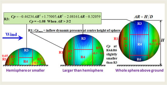
This section provides suggestions for wind-resistant design of spherical structures based on the results. In the Japanese code governing the design of spherical structures [27], the whole surface of a dome structure (including the truncated hemisphere) with a rise–span ratio of less than 0.5 is divided into four regions to obtain separate mean pressure coefficients for wind-resistant design. Similar to the aforementioned Japanese code, this study divided the surface of a sphere into six regions (Figure 14). Region R1, which is located at the windward surface, is subjected to strong positive pressure due to the impinging effect of wind. Region R2 is the transition area from positive to negative pressures, and zero pressure is appropriate. The position of R2 can be determined according to the position angle of zero pressure shown in Figure 10. R3 (top region) and R4 (two side regions) are subjected to a strong suction effect, and the largest negative pressure appears in R3. R5 covers a large area of the rear surface but is not consequential for wind-resistant design because the wind pressure in this region is small. If the inflow dynamic pressure at the apex height H is used as a reference, a Cp value of −0.3 to 0.3 is recommended for R5. The bottom region R6 and its two small adjacent regions only exist when the spherical structure is a whole sphere. To develop a wind-resistant design for a spherical structure, determining the maximum positive pressure acting on the windward wall and the maximum negative pressures at the top region are important. When the spherical structure is equal to or smaller than a hemisphere, a Cp value of 0.6–0.7 is suggested for R1. For structures larger than a hemisphere, the pressure in R1 can be obtained from the inflow dynamic pressure at the centre height of the sphere because the inflow dynamic pressure changes to being static pressure near this height according to Bernoulli’s theorem. For all types of spherical structures, if the inflow dynamic pressure at the apex height H is used as a reference, the polynomial approximation equation presented in this study (Equation (11)) is suggested for evaluation of Cp in R3. The limitations of using Equation (11) arise from the limited number of simulation models in which a whole sphere is located above the ground. As shown in Figure 11, the change in the area-averaged Cp value in the top region was small for Models 16–18. Therefore, when a whole sphere is located far from the ground, a Cp value of −1.08 is suggested for R3. A Cp value smaller than that in R3 is appropriate for the side region R4 and bottom region R6. In an actual project, a support structure is usually connected to R6 when a whole sphere is located above the ground. As a result, the pressure acting on R6 may be affected by the support structures.

6. Conclusions

In this study, four RANS turbulence models that are commonly used in wind engineering were evaluated with respect to prediction of the mean wind loads acting on a hemisphere. The best turbulence model (SST k–ω model) was selected to investigate the wind pressures acting on various types of spherical structures with different ARs. Design suggestions were presented based on the obtained results.

The results indicated that, in a large area of the windward surface, the pressures were positive due to the impinging effect of wind. The maximum positive pressure gradually increased with AR. The largest positive Cp was 0.6–0.7 for a hemisphere and for structures smaller than a hemisphere. For structures larger than a hemisphere, the largest positive pressure nearly equalled the inflow dynamic pressure at the centre height of the sphere. The structures were subjected to a strong suction effect at the crown of the sphere as well as its two side and bottom regions (if they exist). This strong suction effect gradually strengthened as AR increased. For a whole sphere located above the ground, the suction effect at the side and bottom regions was strong and only marginally weaker than that at the top region. The strongest suction effect occurred at the apex position in all the models. In most regions of the rear surface, the pressure was small. By using the inflow dynamic pressure at the apex height as a reference in each case, the negative Cp over the crown area was averaged. Moreover, a polynomial approximation function was derived for quickly determining the strongest suction effect for all types of spherical structures.

The drag coefficient C_D increased rapidly with AR and reached its maximum value when the structure was close to a whole sphere. Subsequently, the C_D value suddenly decreased because of the appearance of negative pressures in the lower part of the windward wall and large-area positive-pressure regions at the rear surface. The total lift coefficient C_L increased rapidly with AR and reached its maximum value in Model 9. C_L suddenly decreased in Model 12 because of the appearance of a strong suction effect at the bottom of the structure. The strong suction effect acting on the top area contributed considerably to total lift. For a whole sphere located far from the ground, the changes in both C_D and C_L were small.

Based on the obtained results, suggestions were proposed for wind-resistant design of spherical structures. This study had its limitations, suggesting future work. The predicted result by the RANS model was not satisfactory in a small leeward region. More simulation models are still necessary to be conducted to generalize the results.

References

1. Lin, N.; Letchford, C.; Tamura, Y.; Liang, B.; Nakamura, O. Characteristics of wind forces acting on tall buildings. J. Wind Eng. Ind. Aerodyn. 2005, 93, 217–242. [Google Scholar] [CrossRef]
2. Jiang, G.; Yoshie, R. Side ratio effects on flow and pollutant dispersion around an isolated high-rise building in a turbulent boundary layer. Build. Environ. 2020, 180, 107078. [Google Scholar] [CrossRef]
3. Cheng, C.M.; Fu, C.L. Characteristic of wind loads on a hemispherical dome in smooth flow and turbulent boundary layer flow. J. Wind Eng. Ind. Aerodyn. 2010, 98, 328–344. [Google Scholar] [CrossRef]
4. Toy, N.; Moss, W.D.; Savory, E. Wind tunnel studies on a dome in turbulent boundary layers. J. Wind Eng. Ind. Aerodyn. 1983, 1, 201–212. [Google Scholar] [CrossRef]
5. Savory, E.; Toy, N. Hemisphere and hemisphere-cylinders in turbulent boundary layers. J. Wind. Eng. Ind. Aerodyn. 1986, 23, 345–364. [Google Scholar] [CrossRef]
6. Tavakol, M.M.; Yaghoubi, M. Experimental and Numerical Analysis of Turbulent Air Flow Around a Surface Mounted Hemisphere. Sci. Iran. 2010, 17, 480–491. [Google Scholar]
7. Tavakol, M.M.; Abouali, O.; Yaghoubi, M. Large eddy simulation of turbulent flow around a wall mounted hemisphere. Appl. Math. Model. 2015, 39, 3596–3618. [Google Scholar] [CrossRef]
8. Kharoua, N.; Khezzar, L. Large eddy simulation study of turbulent flow around smooth and rough domes. Proc. Inst. Mech. Eng. Part C J. Mech. Eng. Sci. 2013, 227, 2686–2700. [Google Scholar] [CrossRef]
9. Wu, P.; Chen, G.; Feng, R.; He, F. Research on Wind Load Characteristics on the Surface of a Towering Precast Television Tower with a Grid Structure Based on Large Eddy Simulation. Buildings 2022, 12, 1428. [Google Scholar] [CrossRef]
10. Meroney, R.N.; Letchford, C.W.; Sarkar, P.P. Comparison of numerical and wind tunnel simulation of wind loads on smooth, rough and dual domes immersed in a boundary layer. Wind Struct. 2002, 5, 347–358. [Google Scholar] [CrossRef]
11. Yousef, M.A.; Selvam, P.R.; Prakash, J. A comparison of the forces on dome and prism for straight and tornadic wind using CFD model. Wind Struct. 2018, 26, 369–382. [Google Scholar]
12. Li, T.T.; Yan, G.R.; Yuan, F.P.; Chen, G.D. Dynamic structural responses of long-span dome structures induced by tornadoes. J. Wind. Eng. Ind. Aerodyn. 2019, 190, 293–308. [Google Scholar] [CrossRef]
13. Tsutsui, T. Flow around a sphere in a plane turbulent boundary layer. J. Wind. Eng. Ind. Aerodyn. 2008, 96, 779–792. [Google Scholar] [CrossRef]
14. Sadeghi, H.; Heristchian, M.; Aziminejad, A.; Nooshin, H. Wind effect on grooved and scallop domes. Eng. Struct. 2017, 148, 436–450. [Google Scholar] [CrossRef]
15. Taylor, T.J. Wind pressures on a hemispherical dome. J. Wind. Eng. Ind. Aerodyn. 1991, 40, 199–213. [Google Scholar] [CrossRef]
16. Chen, Z.; Su, Y.; Wang, J.; Su, N.; Tang, L. Experimental Study on Aeroelastic Instability of Spherical Inflatable Membrane Structures with a Large Rise–Span Ratio. Buildings 2022, 12, 1336. [Google Scholar] [CrossRef]
17. Uematsu, Y.; Yamada, M.; Inoue, A.; Hongo, T. Wind loads and wind-induced dynamic behaviour of a single-layer latticed dome. J. Wind. Eng. Ind. Aerodyn. 1997, 66, 227–248. [Google Scholar] [CrossRef]
18. Sun, Y.; Qiu, Y.; Wu, Y. Modeling of Wind Pressure Spectra on Spherical Domes. Int. J. Space Struct. 2013, 28, 87–99. [Google Scholar] [CrossRef]
19. Park, M.J.; Yoon, S.W.; Kim, Y.C.; Cheon, D.J. Wind Pressure Characteristics Based on the Rise–Span Ratio of Spherical Domes with Openings on the Roof. Buildings 2022, 12, 576. [Google Scholar] [CrossRef]
20. Orszag, S.A.; Yakhot, V.; Flannery, W.S.; Boysan, F.; Patel, B. Renormalization Group Modeling and Turbulence Simulations. In Proceedings of the International Conference on Near-Wall Turbulent Flows, Tempe, AZ, USA, 15–17 March 1993. [Google Scholar]
21. Kato, M.; Launder, B.E. The modelling of turbulent flow around stationary and vibrating square cylinders. In Proceedings of the Ninth Symposium on Turbulent Shear Flows, Kyoto, Japan, 16–18 August 1993. [Google Scholar]
22. Menter, F.R. Two-Equation Eddy-Viscosity Turbulence Models for Engineering Applications. AIAA J. 1994, 32, 1598–1605. [Google Scholar] [CrossRef] [Green Version]
23. Mochida, A.; Tominaga, Y.; Murakami, S.; Yoshie, R.; Ishihara, T.; Ooka, R. Comparison of various k–ε models and DSM applied to flow around a high-rise building -report on AIJ cooperative project for CFD prediction of wind environment. Wind. Struct. 2002, 5, 227–244. [Google Scholar] [CrossRef] [Green Version]
24. Tominaga, Y.; Mochida, A.; Murakami, S.; Sawaki, S. Comparison of various revised k-ε models and LES applied to flow around a high-rise building model with 1:1:2 shape placed within the surface boundary layer. J. Wind. Eng. Ind. Aerodyn. 2008, 96, 389–411. [Google Scholar] [CrossRef]
25. Yang, W.; Quan, Y.; Jin, X.Y.; Tamura, Y.; Gu, M. Influences of equilibrium atmosphere boundary layer and turbulence parameter on wind loads of low-rise buildings. J. Wind. Eng. Ind. Aerodyn. 2008, 96, 2080–2092. [Google Scholar] [CrossRef]
26. Tominaga, Y.; Mochida, A.; Yoshie, R.; Kataoka, H.; Nozu, T.; Yoshikawa, M.; Shirasawa, T. AIJ guidelines for practical applications of CFD to pedestrian wind environment around buildings. J. Wind. Eng. Ind. Aerodyn. 2008, 96, 1749–1761. [Google Scholar] [CrossRef]
27. Architectural Institute of Japan (AIJ). AIJ Recommendations for Loads on Buildings; AIJ: Tokyo, Japan, 2004. [Google Scholar]
Figure 1. Comparisons of mean pressure coefficient Cp along the centre meridian of the hemisphere under a smooth inflow condition [3].
Buildings 12 01832 g001
Figure 2. Comparisons of mean streamlines and normalised turbulent kinetic energy obtained with the adopted models in the centre plane of the domain.
Buildings 12 01832 g002
Figure 3. Simulation models.
Buildings 12 01832 g003
Figure 4. Computational domain and the mesh distribution.
Buildings 12 01832 g004
Figure 5. Comparisons of the mean pressure coefficient obtained in different studies along the centre meridian of a hemisphere in a turbulent boundary layer [3,5,8].
Buildings 12 01832 g005
Figure 6. Mean pressure coefficient on the surface of sphere and in the centre plane of the domain (reference height: 10 m): (a) Model 2; (b) Model 4; (c) Model 6; (d) Model 8; (e) Model 10; (f) Model 12; (g) Model 14; (h) Model 16; (i) Model 18.
Buildings 12 01832 g006
Figure 7. Mean streamlines and normalised mean streamwise velocity (U/U10) in the centre plane of the domain: (a) Model 2; (b) Model 4; (c) Model 6; (d) Model 8; (e) Model 10; (f) Model 12; (g) Model 14; (h) Model 16; (i) Model 18.
Buildings 12 01832 g007
Figure 8. Mean pressure coefficient along the centre meridian of the upper hemisphere (reference height: H).
Buildings 12 01832 g008
Figure 9. Definition of γ for nonhemispherical structures: (a) smaller than hemisphere; (b) larger than hemisphere.
Buildings 12 01832 g009
Figure 10. Position angles of the maximum positive Cp and zero Cp in the windward wall.
Buildings 12 01832 g010
Figure 11. Point-maximum negative Cp and area-averaged Cp over the top region (reference height: H).
Buildings 12 01832 g011
Figure 12. Variations in drag coefficient with the model number.
Buildings 12 01832 g012
Figure 13. Variations in lift coefficient with the model number.
Buildings 12 01832 g013
Figure 14. Suggested regional divisions for the wind loads on a spherical structure: (a) top view; (b) side view.
Buildings 12 01832 g014