Evaluation of Indoor Thermal Environments Using a Novel Predicted Mean Vote Model Based on Artificial Neural Networks

Abstract

The assessment of indoor thermal environments is crucial to achieving thermal comfort and energy efficiency. However, the inaccurate evaluation and strong nonlinear variations of thermal comfort parameters limit engineering designs. Therefore, a coupled heat-transfer model was developed in this study, and large eddy simulations were performed to verify the influence of inertia and buoyancy—which are mutually exclusive forces but coexist in large-space building environments—on inhomogeneous thermal environments. Furthermore, an artificial neural network (ANN) model was designed to overcome the limitations of the nonlinear relationships between thermal parameters and predicted mean vote (PMV) values. PMV indexes can be predicted using the ANN model when thermal parameters are used as input data. Subsequently, a genetic algorithm, harmony search algorithm, gravitational search algorithm, and whale optimization algorithm were adopted to optimize the neural network structure to prevent its confinement in a local optimum. Finally, with 5000 data sets, the minimum-error neural network structure 6-22-23-1 of the ANN-GA neural network model had high prediction accuracy, mean relative error < 1.38, root mean square error < 1.34, and a regression coefficient of ~1. The proposed ANN model can help improve the assessment of the thermal environment and thermal comfort of buildings.

1. Introduction

With continuously improving living standards, the quality requirements for indoor living environments have increased. A comfortable indoor thermal environment not only promotes a good quality of life but also increases work efficiency [1,2,3,4]. Therefore, assessing human thermal comfort is crucial to improving people’s lives and the energy efficiency of buildings. Hensen defined thermal comfort as a state wherein environmental temperature or human behavior need not be modified for comfort [5]. The American Society of Heating, Refrigerating, and Air-Conditioning Engineers (ASHRAE) describes thermal comfort as a psychological state of satisfaction with the temperature of an environment [6]. Thus, thermal comfort is not only a physical state but also a cognitive state and is influenced by several factors, such as physiology, space, and room temperature [7]. It is an indispensable tool for the holistic assessment of a thermal environment [8]. Conventionally, thermal discomfort is considered a subjective condition, whereas thermal sensation is considered an objective condition [9]. Satisfaction in a thermal environment is a complex subjective response to several interactive and less distinct variables [10]. In 1962, Macpherson proposed that the following six factors influence thermal sensation: four physical variables (air temperature, air velocity, relative humidity, and mean radiant temperature) and two personal variables (clothing insulation and metabolic rate) [5]. The factors that influence thermal comfort can be used to determine energy consumption by systems in building environments; these factors are crucial to the sustainability of buildings [11]. Thermal comfort is a key parameter for a healthy and efficient workplace [12,13].

Human comfort is closely related to the thermal environment of a room; thus, the heat transfer characteristics of the room are important and should be accurately evaluated. Thermal comfort is typically described using extended heat transfer models that account for environmental and human parameters. Van Hoof et al. [14] reviewed thermal comfort models and their applications between the late 1990s and 2010. Van Hoof et al. [15] reviewed modeling methods to simulate adaptation to thermal environments. Croitoru et al. [16] discussed human physiological and mental models of adaptation to environmental temperature; they proposed the use of human thermoregulation models in combination with numerical methods of computational fluid dynamics (CFD) to effectively assess thermal comfort. Djongyang et al. [17] reviewed mathematical models that account for conduction, convection, radiation, humidity, clothing insulation, and metabolism. Cheng et al. [18] evaluated the thermal characteristics of an indoor environment by using human thermal comfort parameters and a CFD model, which represented the distribution patterns of macroscopic airflow and air temperature but neglected small-scale turbulence characteristics. Chen analyzed and compared experimental models, small-scale empirical models, large-scale empirical models, multizonal network models, a partitioning model, and a CFD model [19]. Furthermore, the reliability and accuracy of turbulence models were improved and CFD models were integrated with building simulation models. Fu et al. [20] reviewed various human thermoregulation models and noted the importance of initial indoor boundary parameters. All aforementioned studies were focused on the effects of individual variables on the thermal environment. However, practical indoor thermal characteristics are determined using a multiphysical coupled field comprising convection, conduction, and radiation. Highly accurate mathematical models of coupled heat transfer are necessary for representing actual physical fields, and the accuracy of numerical simulations should be improved to capture small-scale turbulence characteristics. Therefore, research should be focused on developing new approaches, especially for conventional turbulence models. It is known that advanced numerical simulation methods can yield detailed and highly accurate information regarding heat transfer in the case of small-scale flow.

In 1970, Fanger proposed a predictive mean vote (PMV) prediction model based on statistical analysis [21]. The model accounted for parameters such as air temperature, humidity, airflow velocity, mean radiant temperature, clothing insulation, and human metabolic rate. Studies have demonstrated that the PMV prediction model can be used to accurately evaluate thermal comfort at steady state [22]. Several researches have used the model to evaluate thermal comfort. Overall, physical and human factors are the key variables that determine thermal comfort in indoor environments. The control methods used to improve thermal comfort depend on all the input variables of control systems. Predicting the associated outputs can be effective for designing suitable control strategies to assess and improve thermal comfort. However, the strong nonlinear relationship between the system input parameters and the results is a limitation, and conventional methods are ineffective at revealing intrinsic relationships between the variables.

In recent decades, neural network technology has been increasingly used in various fields [23]. Combined with engineering techniques, this technology can map the relationship between input and output elements [24]. Shaikh et al. [25] proposed a classification method that accounted for conventional, model-based, and intelligent control systems with predictive or adaptive controllers; they also proposed thermal comfort models based on artificial intelligence techniques [26]. Afram and Janabi–Sharifi [27] reviewed a data-driven, physical, and grey box-based HVAC system. Dounis and Caraiscos [28] discussed intelligent computational methods such as fuzzy logic-based methods, neural networks, and hybrid methods to construct high-precision models of thermal comfort. Wang and Srinivasan [29] reviewed the concepts, applications, advantages, and disadvantages of artificial intelligence-based prediction methods. The current challenges include the tendency of neural networks to fall into local optimization and the lack of accuracy of models.

According to the aforementioned studies, different initial boundary parameters can influence the airflow and temperature fields in a room, and highly accurate numerical simulation methods should be developed to assess the characteristics of small-scale turbulence in indoor environments. Furthermore, the models of multiphysical coupled heat transfer (convection, conduction, and radiation) in indoor environments have limitations. The influence of different initial boundary conditions on indoor airflow and temperature fields in a specific room should be investigated, and the correlation between the indoor thermal environment and human comfort should be explored. With advancements in the field of artificial intelligence, the accuracy of intelligent thermal comfort prediction models improves, and models that combine thermal comfort parameters and artificial intelligence can be further improved.

To address the aforementioned limitations, we used an advanced high-precision large eddy simulation (LES) method that accounts for turbulent small vortex motion and portrays realistic indoor information. The method can provide insights into heat flow and heat transfer. In addition, artificial intelligence controls the strong nonlinear variation in each parameter in the thermal comfort prediction model, decouples the correlations among the parameters, and reveals the intrinsic relationships among the variables. The predicted correlated outputs can be used to effectively design suitable control strategies to assess and improve thermal comfort; the results can also provide guidance for further research. To address the aforementioned limitations, the remainder of this paper is organized as follows: Section 2 discusses the main methods used to determine thermal sensation and comfort. Section 3 describes the basic parameters used for assessing thermal comfort in indoor spaces, with a particular focus on the parameters that determine relevant temperatures. Section 4 describes thermal comfort indexes used to assess various thermal environments and conditions. Section 5 discusses the thermal comfort models that can be employed to develop strategies for controlling indoor thermal environments. Section 6 entails the conclusions of the study.

2. Thermal Comfort Model

Thermal environments are typically assessed in terms of thermal comfort, which is a key factor for the subjective evaluation and perception of indoor thermal environments. A comfortable indoor environment induces physical and psychological pleasure and relaxation [30]. Factors that primarily influence human thermal comfort include subjective human feelings, such as mood and emotion, and thermal environment factors, such as indoor humidity and temperature. Thermal comfort is also influenced by differences between the insulation afforded by the clothing of different individuals and between the different physiological metabolic rates of the individuals. Human sensitivity to the environment is influenced by a combination of these factors, which cause an individual to feel physically comfortable [31].

2.1. Thermal Comfort Index

Typically, human thermal comfort is primarily influenced by six factors [32,33].

(i) Air temperature

The most intuitively perceived factor of an indoor environment is temperature; thermoregulation is the primary response of the human body to variations in temperature in an indoor environment. Notably, when the indoor temperature is <12 °C or >30 °C, the functional state of the human body is affected, especially the operation of the blood circulatory and digestive systems. At such temperatures, an individual cannot be comfortable or perform regular tasks. When the room temperature is lower than 18 °C or higher than 28 °C, the individual’s work efficiency is affected. The most comfortable indoor temperature is 25 °C, which is associated with the highest work efficiency.

(ii) Relative humidity

Relative humidity also has notable influence on human comfort. At a given indoor temperature, the higher the relative humidity, the higher the water vapor pressure in the air, and the less the amount of sweat excreted by the body. Moreover, when the relative humidity increases, high temperature causes suffocation, and low temperature causes individuals to feel cold. Humidity influences the evaporation and diffusion of sweat from the skin surface, and skin temperature changes when the skin relaxes or contracts during evaporation.

(iii) Airflow velocity

The velocity of airflow directly affects the rate of heat dissipation and the evaporation of sweat. The optimal airflow velocity is determined by the movement of the human body. When an individual moves fast, thermal comfort is achieved if airflow velocity is high; however, when the individual moves slow or is not moving, the airflow velocity required for thermal comfort is low. Effectively, airflow velocity depends on the rate of evaporation of sweat from the surface of the human body.

(iv) Average radiation temperature

The average radiation temperature is the average temperature of the radiation emitted by surrounding objects in an indoor environment; it has an influence on human thermal comfort. The exchange of radiated heat between the human body and the surfaces of objects in the environment depends on the radiation emitted from each surface and the relative positions of individuals and objects. The average radiation temperature can be measured using a black ball thermometer.

(v) Human metabolic rate

Metabolism is the process that involves the conversion of matter into energy in living organisms; it is a process of chemical heat production, which results in chemical changes in living organisms. The metabolic rate of the human body is determined by the amount of heat generated per unit of time on the surface area of the body. The unit of metabolic rate is met; 1 met = 58.2 W/m². Metabolic rate increases with an increase in activity. For example, the metabolic rate of the human body is 1 met when sitting still, ~0.7 met when lying down, and 7.6 met when playing ball. The amount of heat generated by the human body is different in different states, and the metabolic rate of the human body is also a key factor affecting thermal comfort.

(vi) Clothing insulation

In addition to other factors, the clothing of an individual has an influence on thermal comfort. For example, during summer, people typically wear light clothes such as short-sleeved clothes, which dissipate heat and provide comfort, whereas during winter, people wear thicker clothes that provide high thermal insulation and comfort and protect the body from low environmental temperatures. Therefore, suitable clothing can help regulate thermal comfort. Clothing is generally distinguished according to the degree of insulation; suitable clothing insulation ranges from 0.35 to 0.6 clo during summer and from 0.8 to 1.2 clo during winter.

The six main factors that influence thermal comfort can be categorized as physical environmental variables (air temperature, relative air humidity, air velocity, and average radiation temperature) and human factors (human metabolic rate and clothing insulation). If metabolic rate and clothing insulation are known and the environmental variables are appropriately regulated, an optimized combination of these variables can be used to calculate the health-friendliness and thermal comfort of indoor environments; the criteria for evaluating these parameters are defined as the comfort rating index.

2.2. Thermal Comfort Equations

Prof. Fanger from Denmark developed the PMV model [21] based on subjective voting and testing of environmental parameters, which influence physiological thermal sensation. The PMV index is commonly used to assess indoor thermal environments. The PMV index uses a seven-point scale (−3, −2, −1, 0, +1, +2, and +3) corresponding to seven degrees of thermal sensation in the human body: cold, cool, slightly cool, neutral, slightly warm, warm, and hot. In addition, differences in physical strength and the ability to withstand high or low temperatures influence the degree of thermal comfort of people in indoor environments. To evaluate these differences, Prof. Fanger formulated a predicted percentage dissatisfaction (PPD) index, which can be used to predict the effects of thermal environments on the human body, as displayed in

Table 1. PMV–PPD scale.

Thermal Sensation	PMV	PPD (100%)
Hot	+3	100
Warm	+2	75
Slightly warm	+1	25
Neutral	0	5
Slightly cool	−1	25
Cool	−2	75
Cold	−3	100

. For a comfortable thermal environment, the generally acceptable range for PMV is from −1.0 to 1.0, with PPD < 26% [21].

Prof. Fanger developed a thermal comfort model, which describes energy balance in the human body. The PMV equation for the expected heat index is as follows:

$$\begin{gathered} \mathrm{PMV}=\left(0.303e^{-0.036M}+0.028\right)\{M-W-3.05\times {10}^{-3}\times \left[5733-6.99\left(M-W\right)-Pa\right] \\ -0.42\left[\left(M-W\right)-58.15\right]-1.72\times {10}^{-5}M\left(5867-Pa\right)-0.0014M\left(34-t_a\right) \\ -3.96\times {10}^{-8}{f}_{cl}\left[{\left(t_{cl}+273\right)}^4-{\left(t_r+273\right)}^4-f_{cl}{h}_c\left(t_{cl}-t_a\right)\right]\} \end{gathered}$$

(1)

The important parameters are as follows:

• M: energy metabolic rate of the body in W/m².
• W: mechanical power generated by the human body in W/m².
• Pa: partial pressure of water vapor in the surrounding air in Pa.
• t_a: temperature of the air around the human body in °C.
• t_r: average radiation temperature in °C.
• f_cl: ratio of the area of the body covered by clothing to the exposed area.
• t_cl: temperature of the outer surface of the garment in °C.
• h_c: surface heat transfer coefficient in W/(m²·K).

Accordingly, Prof. Fanger derived the following expression using PMV and PPD along with the quantitative evaluation of the sampling statistics.

$$PPD=100-95exp\left[-\left(0.03353PM{V}^4+0.2179PM{V}^2\right)\right]$$

(2)

As illustrated in Equation (2), the PMV–PPD equation for the expected heat index is a complex multiparameter and multivariate nonlinear expression, which can be indirectly transformed using relevant parameters into a PMV equation for the expected heat index to calculate PMV values.

The surface temperature of clothing, t_cl, is calculated using the following equation:

$$\begin{array}{l}{t}_{cl}=35.7-0.028\left(M-W\right)-I_{cl}\\ \begin{array}{cc}& \end{array}\times \left\{3.96\times {10}^{-8}{f}_{cl}\left[{\left(t_{cl}+273\right)}^4-{\left(t_r+273\right)}^4-f_{cl}{h}_c\left(t_{cl}-t_a\right)\right]\right\}\end{array}$$

(3)

The surface heat transfer coefficient, h_c, is calculated as follows:

$$h_c=\{\begin{array}{ll}2.38{\left(t_{cl}-t_a\right)}^{0.25},& if 2.38{\left(t_{\mathrm{cl}}-t_a\right)}^{0.25}\ge 12.1\sqrt{Va}\\ 12.1\sqrt{Va},& if 2.38{\left(t_{\mathrm{cl}}-t_a\right)}^{0.25}<12.1\sqrt{Va}\end{array}$$

(4)

where Va is the airflow velocity, m/s. The clothing coefficient f_cl is calculated using the following formula:

$$f_{cl}=1.0+0.3I_{cl}$$

(5)

where I_cl is the clothing insulation. The water vapor partial pressure in the air surrounding the body is calculated as follows:

$$Pa={10}^{-5}\varphi \exp \left[-5800/t_a+0.048Ta+4.1\times {10}^{-8}{t}_a{}^3+6.545\ln Ta\right]$$

(6)

where φ is the relative humidity; Ta = t_a + 273.15 (K).

The equation for the average indoor radiation temperature t_r is as follows:

$$t_r=t_g+2.4V{a}^{0.5}\left(t_g-t_a\right)$$

(7)

where t_g is the temperature of the black sphere, which is typically 2–3 °C higher than room temperature. Substituting Equations (3)–(7) into Equation (1), the PMV equation for the compound heat index can be simplified as follows:

$$\mathrm{PMV}=f\left(M,f_{cl},t_a,t_r,Va,\phi \right)$$

(8)

Based on Equation (8), the PMV thermal comfort index for evaluating indoor thermal comfort was established in this study. In addition, the influence of the initial thermal environmental variables and human factors on PMV was investigated. Therefore, the present study lays a foundation for the subsequent modeling of a neural network based on PMV prediction.

3. Modeling Process

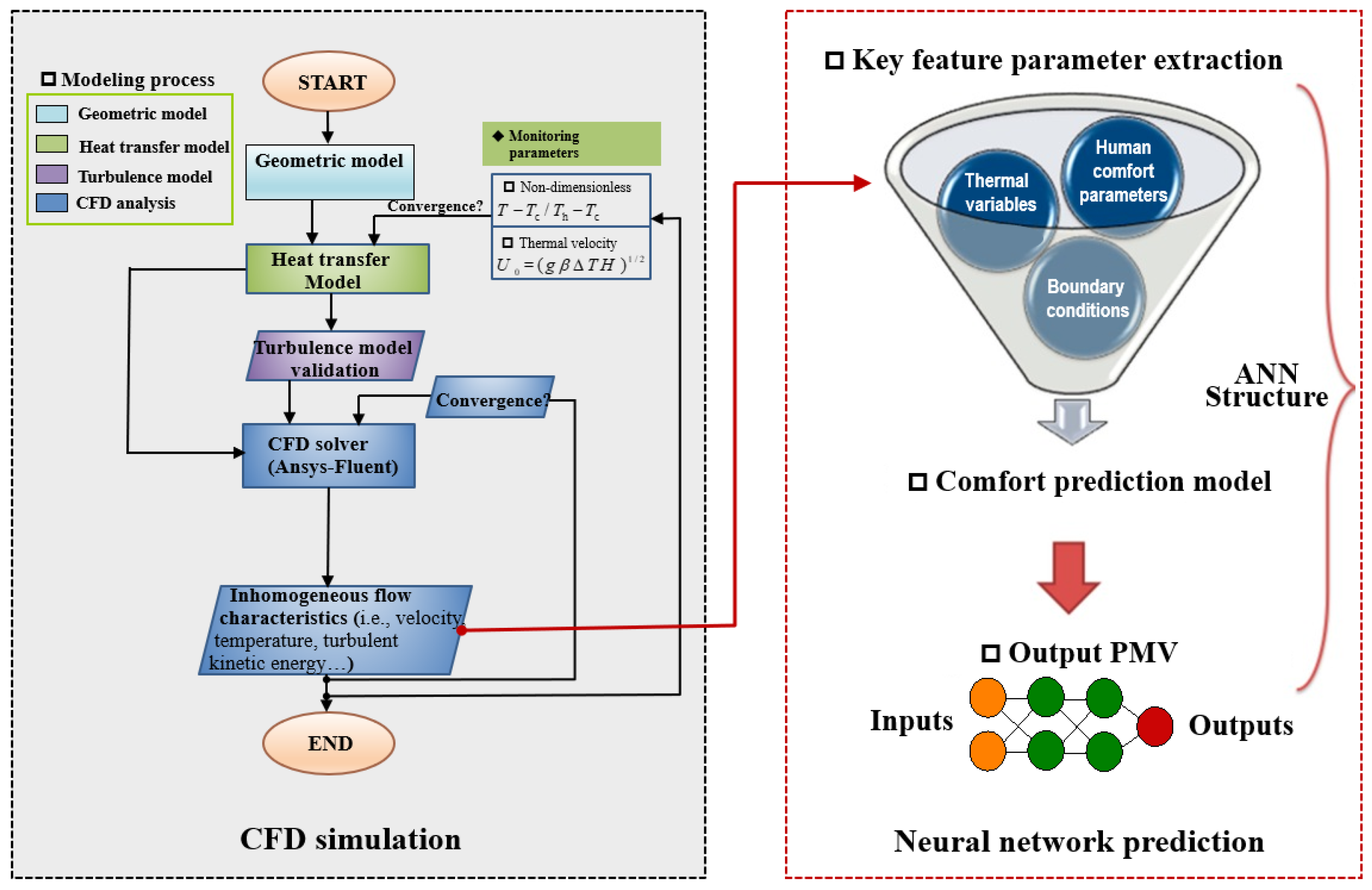
Thermal comfort prediction is a complex nonlinear process that is directly influenced by multiple factors. Therefore, constructing a mathematical model for thermal comfort prediction is necessary. Figure 1 illustrates the modeling process, which involved two main stages: numerical simulation and neural network prediction. In the model, the thermal environment was represented by an extremely complex airflow phenomenon, which was modeled through CFD techniques. In addition, parameters having substantial effects on the PMV indexes were identified from the numerical simulation results and used as input elements to construct a neural network prediction model.

3.1. Geometrical Model

Figure 2a depicts the overall office building model constructed for numerical simulations; the building is subjected to uniform lighting during all seasons. We analyzed only the indoor thermal environment of the building, with only solar radiation as the heat source. The model was constructed considering that the building may be located in a rural or urban area, with or without vegetation outside. The proposed physical model is universally applicable. Figure 2b depicts a representative room configuration with a primary structure constituted by an insulated floor, roof, three walls, and a thermally conductive glass curtain wall. One of the walls has openings for air ventilation, and the glass allows external sunlight radiation to enter and induce heat in the room. Figure 2c depicts the physical model of the simulated thermal environment, with dimensions 3 m, 2.5 m, and 3 m along the x, y, and z-axis directions, respectively.

3.2. Heat Transfer Model

Figure 3 displays a schematic of the heat transfer model. The process of heat transfer strictly obeys the law of energy conservation. Solar radiation is the primary form of heat in the model; the heat transfer processes include conduction, convection, and radiation. The proposed model is focused on the airflow field in a room. For modeling purposes, the term representing radiation from the glazing can be completely converted into the heat load term in the expression for thermal radiation displayed in Figure 3b. Glazing is a heat transfer medium that dominates heat exchange between the internal and external walls in the model.

The inner wall temperature is obtained according to the following equation:

$$\underset{\mathrm{Radiation}}{\underbrace{{\alpha }_s{G}_s}}=\underset{\mathrm{Convection}}{\underbrace{h_{in}(T_{\mathrm{w},\mathrm{in}}-T_{\mathrm{f},\mathrm{in}})}}+\underset{\mathrm{Radiation}}{\underbrace{\sigma \epsilon (T_{{{}_{\mathrm{w},\mathrm{o}}}_{\mathrm{ut}}}^4-T_{{}_{\mathrm{f},\mathrm{out}}}^4)}}+\underset{\mathrm{Convection}}{\underbrace{h_{\mathrm{out}}(T_{\mathrm{w},\mathrm{out}}-T_{\mathrm{f},\mathrm{out}})}}$$

(9)

$$\underset{\mathrm{Conduction}}{\underbrace{\frac{\lambda }{\delta }(T_{\mathrm{w},\mathrm{out}}-T_{\mathrm{w},\mathrm{in}})}}=\underset{\mathrm{Convection}}{\underbrace{h_{\mathrm{in}}(T_{\mathrm{w},\mathrm{in}}-T_{\mathrm{f},\mathrm{in}})}}$$

(10)

where G_s is the incoming solar radiation and α_s is the absorption coefficient; h is the convective heat transfer coefficient; σ is Stefan–Boltzmann constant, which has a value of 5.672 × 10⁻⁸ W/m²·K; T_w,in and T_w,out denotes the inner and outer wall temperatures, respectively. The term representing the radiation from the glass can be neglected because the amount of radiation is negligible compared with the amount of heat transferred through internal convection. A mixed heat transfer equation is derived using Equations (9) and (10):

$${\alpha }_{\mathrm{s}}{G}_s=\frac{\lambda }{\delta }(T_{\mathrm{w},\mathrm{out}}-T_{\mathrm{w},\mathrm{in}})+h_{\mathrm{out}}(T_{\mathrm{w},\mathrm{out}}-T_{\mathrm{f},\mathrm{out}})$$

(11)

The statistical values of thermal conductivity and average outdoor air temperature of glass are displayed in

Table 2. Parameter settings of indoor and outdoor air temperatures and glass properties.

Thermal Boundary Parameters	Specific Values
αs	0.85
Gs (W/m2)	3000
hout (W/m2·K)	220
Tf,out (K)	288.15
Tw,out (K)	297.15
Tw,in (K)	295.15
λ (W/m·K)	0.038
δ (mm)	22

.

3.3. Validation of Turbulence Model

The indoor thermal environment in the building significantly influenced human comfort. Thus, multiscale airflow and temperature fields in the indoor environment should be analyzed.

(i) Turbulence model

LES and direct numerical simulation (DNS) are suitable for calculating small vorticity and turbulence statistics for indoor airflow fields [34]. However, the applicability of DNS is limited by its requirement of high mesh quality. Reynolds-averaged Navier–Stokes (RANS) models, which are based on time-averaged equations, are commonly employed in the simulation of engineering flows using turbulence models [35]. Moreover, the prediction performance of RANS models is unstable, and the compatibility between model parameters and experimental or simulated data is unreliable under various conditions. Therefore, we used the LES model in the present study to evaluate the airflow field in an indoor thermal environment. Herein, the classical two-equation turbulence models (standard k-ε, realizable k-ε, SST k-ω), three-equation models (transition k-kl-ω), four-equation models (transition SST, V2f), and seven-equation models (Reynolds stress) were used to compare the predicted values. These turbulence models can be used to predict turbulent airflow by covering almost all basic airflow states.

(ii) Monitoring physical parameters

The simulation results and experimental data were accurately analyzed and compared to obtain the ideal turbulence model. Moreover, the experimental data were selected carefully. The glass heat source and the air supply system contributed to the multiscale turbulent characteristics of the indoor airflow and temperature fields. Therefore, dimensionless temperature parameters (T − T_min/T_max − T_min) were introduced to evaluate and validate the prediction performance of turbulence models.

The experimental data on thermal characteristics were selected according to [36].

Table 3. Initial parameter settings based on the experimental case [36].

Physical Model			Thermal Boundary Conditions
Length [m]	Width [m]	Height [m]	Hot Source [K]	Cold Source [K]
1.45	0.725	0.725	293.15	333.15

lists the dimensions of the test space; the length, width, and height of the test space were 1.45, 0.725, and 0.725 m, respectively. The test space dimensions promoted airflow and heat transfer. Ref. [36] provided a more detailed description.

3.4. Dynamic Equation

The airflow and temperature distribution in a typical office building was numerically simulated using Fluent 19.0 software. The numerical simulations were based on finite volume methods. The developed LES model is based on instantaneous expressions and governed by the laws of conservation of mass, momentum, and energy.

The continuity equation is as follows:

$$\frac{\partial \rho }{\partial t}+\frac{\partial \left(\rho \overline{u_i}\right)}{\partial x_i}=0$$

(12)

where $\overline{u_i}$ is the velocity vector; x_i and t are the coordinate vector and time, respectively.

The momentum equation is as follows:

$$\frac{\partial }{\partial t}\left(\rho \overline{u_i}\right)+\frac{\partial }{\partial x_j}\left(\rho \overline{u_i}\rho \overline{u_j}\right)=\rho \overline{g_i}-\frac{\partial \overline{P}}{\partial x_i}+\frac{\partial {\tau }_{ij}}{\partial x_j}+\frac{\partial {\sigma }_{ij}}{\partial x_j}$$

(13)

where σ_ij is the stress tensor, and τ_ij is the sub-grid stress (SGS).

Energy equation:

$$\frac{\partial \rho \overline{H}}{\partial t}+\frac{\partial }{\partial x_i}\left(\rho \overline{u_i}\overline{H}\right)=\overline{u_i}\frac{\partial \overline{P}}{\partial x_i}+\frac{\partial }{\partial x_i}\left(\lambda \frac{\partial \overline{T}}{\partial x_i}\right)+\frac{\partial }{\partial x_j}\left(\rho \overline{u_j}\overline{H}-\rho \overline{u_{j}H}\right)$$

(14)

where $\overline{H}$ is the enthalpy and λ is the conductivity.

The SGS term can be divided into isotropic and deviatoric terms:

$${\tau }_{ij}=\underset{deviatoric}{\underbrace{{\tau }_{ij}-\frac{1}{3}{\tau }_{kk}{\delta }_{ij}}}+\underset{isotropic}{\underbrace{\frac{1}{3}{\tau }_{kk}{\delta }_{ij}}}$$

(15)

The deviatoric part represents eddy diffusion, which is defined as

$$\underset{deviatoric}{\underbrace{{\tau }_{ij}-\frac{1}{3}{\tau }_{kk}{\delta }_{ij}}}=-2{\mu }_{SGS}\left(S_{ij}-\frac{1}{3}{S}_{kk}{\delta }_{ij}\right),$$

(16)

where S_ij is the strain-rate tensor, and μ_SGS is the sub-grid viscosity.

SGS viscosity is defined as follows:

$${\mu }_{SGS}=\rho L_m^2{\left(2\overline{S_{ij}} \overline{S_{ij}}\right)}^{1/2}$$

(17)

The mixing length L_m is calculated using the following expressions:

$$\{\begin{array}{c}{L}_m=C_s\Delta \\ \Delta =V^{1/3}\end{array}$$

(18)

In addition, C_s is expressed as follows:

$$C_s=\frac{1}{\pi }{\left(\frac{2}{3C_k}\right)}^{3/4}$$

(19)

C_k is assigned a constant value of 1.4.

All simulations in this study were performed using ANSYS Fluent commercial software. The pressure-based isolation algorithm was employed to solve the discretized governing equations. The gradient evaluation method based on Green–Gauss cells was used to simulate the gradients of the convection and diffusion terms in the flow conservation equations, and the standard scheme was used to interpolate the pressure values on each surface. In addition, the bounded central differencing scheme was used to solve the momentum and energy equations. Furthermore, a bounded second-order implicit scheme was used to solve the time-dependent equations.

3.5. Grid Resolution

Table 4. Mesh validation for the four grid systems.

	Case A	Case B	Case C	Case D
y+	<1	<1	<1	<1
L × W × H	35 × 35 × 2500	40 × 40 × 3000	45 × 45 × 3500	50 × 50 × 4000
Elements	3.0 M	4.7 M	7.0 M	9.9 M
Outlet temperature (K)	270	278	286	291
Error (%)	7.2%	4.5%	1.7%	Baseline
Outlet velocity (m/s)	0.33	0.39	0.44	0.45
Error (%)	27%	13%	2%	Baseline

summarizes the mesh generation methods and simulation results of four grid systems. The value of y⁺, which is a refinement parameter for the near-wall region, is restricted to < 1. Figure 4 displays a schematic of the grid system with a growth coefficient of 1.05, which is the same along the x, y, and z directions. This study established novel grid systems with 3.0 M, 4.7 M, 7.0 M, and 9.9 M elements. The initial thermal boundary conditions were fixed as follows: (i) the inlet velocity was 0.5 m/s and temperature was 293.15 K; (ii) the acceleration due to gravity was 9.8 m/s². The outlet temperature and velocity were considered the monitoring parameters, and the results for the 9.9 M system were considered the baseline. As displayed in Table 3, the error percentages of T_out were 7.2%, 4.5%, and 1.7% for the 3.0 M, 4.7 M, and 7.0 M systems, respectively. The error percentages of V_out were 27%, 13%, and 2% for the 3.0 M, 4.7 M, and 7.0 M systems, respectively. After comparative analysis, the 7.0 M grid system was selected for further simulations.

3.6. Comparison Results

Figure 5 illustrates the comparison of the accuracy of temperature prediction of different turbulence models. Considerable variation was noted, especially near the wall region. The fitness degree between the simulation results and experimental data determined the prediction accuracy of the turbulence models, according to which an excellent model can be selected for future studies. Among all the commonly used turbulence models, the LES turbulence model had the optimal prediction accuracy of 97%. The other turbulence models exhibited poor prediction performances with significant deviations, especially in the top region. In the present study, the LES model accurately evaluated the temperature gradient, and the results were consistent with experimental data. Therefore, the LES model was adopted as the suitable simulation model for this study.

4. Results and Discussion

Table 5. Boundary condition settings for the CFD simulation.

Initial Parameter	Specific Values
Airflow inlet velocity, va (m/s)	0–1
Airflow inlet temperature, ta (°C)	−10–40
Airflow inlet humidity, φ (%)	30–70
Average radiation temperature, tr (°C)	10–30
Clothing insulation, Icl (clo)	0–2
Metabolic rate, M (W/m2)	45–240
Acceleration, g (m/s2)	9.8
Outlet boundary	Outflow

displays the initial boundary condition parameter settings. The gas supply represented the inlet boundary, and the outflow represented the outlet boundary.

Table 5 summarizes the boundary conditions that were divided into two categories: (i) environmental factor variables, which included air temperature, relative air humidity, airflow rate, and average radiation temperature; (ii) human factor variables, which included human metabolic rate and clothing insulation. According to the range of values of environmental factor variables listed in

Table 6. Initial boundary conditions for numerical simulation.

	Inlet Velocity, va (m/s)			Inlet Temperature, ta (°C)			Inlet Humidity, φ (%)
Case 1	0.3			1			30
Case 2		0.5			15			50
Case 3			0.7			25			70

, three cases were established for numerical calculations; the values of initial air temperature, air relative humidity, airflow rate, and average radiation temperature were different in each case. Indoor buoyancy and inhomogeneity caused by gravitational acceleration were evaluated and analyzed in this study.

4.1. Thermal Stratification

The LES turbulence model was employed to investigate three important phenomena under a thermally stratified turbulent airflow in a room: (i) stability criterion of thermal stratification; (ii) inhomogeneity of thermal stratification; and (iii) turbulence statistics of thermal stratification. First, the thermodynamic criterion for the physical stability of thermal stratification in the room was theoretically investigated to derive the theoretical stability equation, and the small-scale thermal stratification phenomenon was evaluated through numerical simulations using the LES model. Second, the influence of thermal stratification on the inhomogeneity of velocity and temperature fields was investigated, and the influence mechanism and potential intrinsic mechanism of thermal stratification were determined. Finally, based on LES data, the turbulent transport characteristics of the thermal stratification phenomenon were analyzed, and the influence of spatial distribution on thermal stratification was investigated. Therefore, a theoretical basis was established for an in-depth understanding of the airflow and heat transfer mechanisms during thermal stratification.

The instability of indoor thermal stratification is a complex problem; thermal stratification is influenced by various factors, including thermal plume, wall boundary layer convection, jet flow of the supplied air, and dynamic thermal characteristics of the building. The determination of the stability of thermal stratification is limited by the combined effects of jet airflow and the dynamic thermal characteristics of the building. However, a complete theory for the determination of the stability of complex indoor thermal stratification is lacking. Considering the uncertainties of the stability of indoor thermal stratification in CFD numerical simulations, the conditions for thermal stratification were derived in this study based on generalized thermodynamic equations. Multiple numerical simulations were performed to analyze the intrinsic mechanism of thermal stratification and the airflow in indoor thermal stratification.

4.2. Turbulent Structure Analysis

Thus far, only a few studies have focused on the factors that lead to the inhomogeneity of indoor environments. The stability of air in an area is determined by the level of turbulence in the air, which primarily results from the interaction of thermal buoyant and inertial forces in the airflow field. Typically, turbulence is weak when thermal buoyant forces dominate, and it is strong when inertial forces dominate. The dimensionless term Ri expresses the relationship between stability and turbulence intensity and is used to determine the turbulence of the airflow field. When Ri is small, the airflow tends to be turbulent, and when Ri is large, the airflow tends to be laminar.

$$Ri=\frac{Gr}{R{e}^2}$$

(20)

The dimensionless terms Gr and Re are the Grashof number and Reynolds number, respectively, and are defined as follows:

$$Gr=\frac{g\beta (T_w-T_b)l^3}{{\nu }^2}$$

(21)

$$Re=\frac{\rho ul}{\mu }$$

(22)

where u and l are the fluid inlet velocity and characteristic length, respectively; β is the volume expansion coefficient, ν and μ are the kinematic viscosity and molecular viscosity, respectively. The influence of natural convection is neglected when Ri < 0.1, and that of forced convection is neglected when Ri > 10; when 0.1 < Ri < 10, mixed convection in a thermally stratified state influences the airflow. The physical model illustrated in Figure 4c has an intermediate symmetry; thus, a two-dimensional plane was selected to evaluate the indoor thermal environment in this study. To determine the average airflow and temperature on the symmetric plane, the mainstream temperature (i.e., average temperature) and the mainstream velocity (i.e., average velocity) are defined as follows:

$$t_b=\frac{{\displaystyle {\int }_{A_c}\rho u{c}_{p}td{A}_c}}{{\displaystyle {\int }_{A_c}\rho u{c}_{p}d{A}_c}}$$

(23)

$$u_b=\frac{{\displaystyle {\int }_{A_c}\rho ud{A}_c}}{{\displaystyle {\int }_{A_c}\rho d{A}_c}}$$

(24)

where A_c is the area of the symmetry plane. Figure 6 displays the histograms of the distribution of Richardson values for Case 1, Case 2, and Case 3. Note that the Richardson number for Case 1 was 12, buoyant airflow was the dominant airflow pattern, and turbulent airflow was negligible. In Case 2, the Richardson number was 0.5, which was between the minimum critical threshold 0.1 and the maximum critical threshold 10; although the airflow exhibited both buoyant and turbulent airflow patterns, turbulent airflow was the dominant flow pattern. In Case 3, the Richardson number was 3, and the airflow was in a mixed mode; however, compared with Case 2, the Richardson number increased to 3, and buoyant airflow was the dominant pattern.

Re denotes the turbulent inertial force field, and Gr denotes the buoyant force field; the statistical properties of the two force fields were further analyzed. The LES results with high Reynolds number values were used to characterize airflow properties. Case 1, Case 2, and Case 3 described in this section were selected to characterize the variations in turbulence with changes in operating conditions. As displayed in Figure 7, the differences in the high Reynolds values were notably under changing operating conditions. In Case 1, when the inlet air was 0.5 m/s, a high Reynolds zone was apparent in the inlet region. The turbulence was suppressed when the air flowed from left to right until the turbulence region disappears. The region on the right side was the region with insignificant turbulence characteristics. In Case 3, the maximum Reynolds number region was concentrated at the inlet when the inlet airflow velocity was 1 m/s. The turbulence was again suppressed near the region on the right. In conclusion, the left and right regions exhibited different airflow characteristics. Velocity distribution was dense near the inlet and the outlet, whereas the turbulence was suppressed in the region on the right. In Case 1, the turbulence characteristics in space were negligible because the inlet airflow velocity was 0.1 m/s.

Buoyant airflow is a physical phenomenon defined by the Grashof number. The formation and trend of buoyant airflow in a room should be carefully evaluated and considered. Figure 8 displays the distribution of Grashof number on the symmetric surfaces in Case 1, Case 2, and Case 3. The buoyant airflow was thermally localized, especially concentrated on the heated glass wall surface. The fluid near the right side indicated apparent thermal stratification. The buoyant force was closely related to the expansion coefficient, as depicted in Equation (21). The density of the fluid increased near the surface of the hot wall, and a buoyancy-driven upward flow of the fluid was apparent in this region. The buoyancy effect was the most pronounced in Case 1, wherein a steady buoyancy effect occurred because of the absence of turbulent airflow at the interior. In Case 2, the inlet temperature was 15 °C, and the inlet velocity was 0.5 m/s. The buoyancy effect was weak because of the turbulence occurring at the interior of the inlet. However, the buoyancy effect was apparent in the region on the right. In Case 3, the inlet temperature was 25 °C, and the inlet velocity was 1 m/s; the intensity of turbulence in the interior increased, and the buoyancy effect was weaker compared with that in Case 2.

Turbulent and buoyant flows had the following characteristics:

(i).

The turbulence at the inlet had a high Reynolds number and high velocity; buoyant airflow mainly occurred at the heated wall surface with thermal stratification.

(ii).

Turbulent and buoyant flows resisted each other and both were mutually exclusive but coexisted in large-space built environments.

4.3. Effects of Different Boundary Conditions on Indoor Thermal Environment

Figure 9a displays that when the airflow velocity was 0.3 m/s, the indoor mainstream airflow was mainly concentrated at the bottom. When the airflow velocity increased to 0.5 m/s, the indoor airflow accelerated and turbulence intensified, while the flow had a vortex structure, and the mainstream airflow occurred in the upward direction. When the airflow velocity was 0.7 m/s, the turbulent force was strong, and the indoor airflow distribution was uniform; however, the airflow was mainly concentrated at the bottom. As displayed in Figure 9b, when the inlet temperature was 1 °C, a high-temperature region was noted in the middle of the interior space and near the right side. The high-temperature region was formed because of a radiant heat source on the inner glass wall surface at the rear side; the heat source heated the critical space fluid and caused an uneven temperature distribution in the chamber. When the temperature increased to 15 °C, a local high-temperature zone occurred on the left side. When the inlet temperature was 25 °C, the temperature distribution in the room was more nonuniform, and the fluid temperature on the rear side was considerably higher than that on the left side. Figure 9c illustrates the cloud plot of indoor humidity distribution; when the inlet humidity was 30%, the indoor humidity was uniform, whereas when the inlet humidity was between 50% and 70%, the indoor humidity distribution was not uniform. Furthermore, the humidity was low in the rear glass radiant heat source area and high in the air away from this area. Overall, the influx and outflux of air on the left side significantly affected indoor airflow distribution. In addition, the rear side glass radiation heat source significantly affected indoor temperature and humidity distribution. Thus, both sides exhibited nonuniform distribution of the airflow field.

4.4. Turbulent Statistical Analysis

Because LES can be used to obtain highly accurate small-scale turbulence structures, this study analyzed the generation of turbulent kinetic energy and buoyancy force. Figure 9 illustrates the distribution of Re and Gr; the region of strong airflow variations located at the left inlet and outlet was dominated by Re. The buoyant force dominated by Gr was concentrated near the right heated wall. The generation of turbulent kinetic energy and buoyant force can be expressed as follows:

$$P_k=-\rho \overline{u_i^{\prime }{u}_j^{\prime }}\frac{\partial u_i}{\partial x_j}$$

(25)

$$P_b=-g\overline{\rho u_j^{\prime }}$$

(26)

In Figure 10a, the distinct peak for a location near the inlet corresponds to the turbulent kinetic energy production rates in Cases 2 and 3, thereby indicating that turbulence changes more significantly near the inlet. Thereafter, a steep drop was observed along the x-axis, corresponding to the strong right-hand buoyancy effect that weakened or suppressed the turbulence. Thus, turbulence is a change in state from turbulent to buoyant flow. In the closed model in Case 1, the inlet velocity was considerably low, and the turbulence generation rate was negligible. In Figure 10b, the peak of the buoyancy generation rate appeared on the right side, indicating that the right heated wall was the origin of the spatial buoyant airflow and thermal stratification. In the closed model in Case 1, the buoyant airflow was fully utilized and relatively stable, such that the peak corresponding to the buoyant effect was the highest. However, when a certain inlet volume was known, the rate of buoyant airflow decreased significantly because of the intervention of turbulence, thereby weakening the buoyant flow.

The radiation from the glass on the right side of the large space acted as a heat source, thereby inducing heat flow in the room. The diffusion of heat has a notable influence on human comfort and combined with the inertial force Re and buoyant force Gr, diffusion induces complex heat transfer. Heat flux can be expressed by the following equation;

$$\rho \left(\overline{u_i{h}_s}-\overline{u_i}\overline{h_s}\right)$$

(27)

The magnitude of the turbulent heat flux (v_x, velocity in the x-axis direction; v_y, velocity in the y-axis direction) determined the degree of turbulent flow. Figure 11a illustrates the turbulent heat flux distribution along the x-axis direction. Notably, the turbulent heat flux increased sharply near the inlet and the outlet: it had the maximum value away from the heated wall. When the inlet velocity was high, the peak heat flow along the x-axis direction was large, indicating a large heat transfer. By contrast, in Case 1, the heat flux along the x-axis direction was almost zero because the airflow velocity was small. Figure 11b illustrates the turbulent heat flux distribution along the y-axis direction. The heat flux distribution along the y-axis direction was drastically different from that along the x-axis. In Case 1, the heat flux perturbation distribution along the y-axis was inhomogeneous in the room, indicating that the degree of heat transfer from the bottom to the top of the room was relatively high. Owing to the small inlet air velocity and strong full-field buoyant force (see Figure 8a), the cold air at the top flowed toward the bottom under the influence of gravity; thus, the heat flux along the y-axis direction was intensified. However, in Case 2 and Case 3, the heat flux on the left side of the x-axis was high and on that of the y-axis was low because of higher inlet airflow velocity along the x-axis. The right side captured the locally enhanced heat flux distribution in the y-axis at the glass radiant heat source mainly because of the heat transfer from the bottom to the top of the buoyancy region, as displayed in Figure 8b,c. In summary, the inertial and buoyant forces have a significant influence on the airflow and temperature fields; however, the influx and outflux of air and the glass heat source resulted in a nonuniform thermal environment, which influenced indoor airflow and temperature distribution and thus, human comfort.

A uniform distribution of indoor temperature is crucial to improving indoor air quality and thermal comfort and is a key factor that effectively improves building environments. We analyzed the indoor airflow velocity, temperature, and humidity distribution. Furthermore, we analyzed the indoor radiant temperature distribution. The complexity of spatial temperature distribution increased because of the presence of glass radiant heat sources. Figure 12 illustrates the points for monitoring indoor space radiation temperature (5 × 9). The interior space was primarily divided into two areas: a turbulence-dominated area at the left air inlet and a buoyancy-dominated area at the right glass wall heat source. The radiation temperature was calculated using the average value of each data point in the space using the following equation:

$$\frac{1}{n}{\displaystyle \sum _{i=1}^n{t}_{\mathrm{r}}}$$

(28)

Under the same operating conditions, the glass wall surface temperature was considerably higher than the indoor radiation temperature, and the difference between the two temperatures determined the flow of radiation. As displayed in Figure 13, the difference between the glass wall surface temperature and the radiation temperature in Case 1 was large because of the low entrance temperature. As displayed in Table 2, the constant temperature of the glass wall surface was 20 °C. When the indoor temperature was increased in Case 2 and Case 3, the difference between the indoor radiation temperature and the glass wall surface temperature was considerably reduced, indicating that the indoor radiation temperature field tended to be consistent. The indoor radiant temperature and the corresponding wall temperature in Case 2 and Case 3 varied similarly from bottom to top, indicating that the radiation temperature distribution in the space is identical.

5. Artificial Neural Networks (ANNs)

Indoor temperature distribution should be regulated to improve indoor air quality, thermal comfort, and thus entire building environments. Several studies on building environment and energy have focused on indoor temperature distribution. Thermal stratification in a building is complex, and analyzing it during airflow is challenging. Moreover, analyzing the complexity of spatial temperature distribution is challenging and is particularly important for the design of building environments. However, when the spatial model and its thermal boundary conditions change, determining temperature distribution through conventional CFD methods is challenging. Therefore, this paper proposes a novel method for predicting spatial temperature field information using data-driven techniques and architectural ANNs.

5.1. Basics of ANNs

An ANN is a complex network structure constituted by a large number of neurons, which are interconnected to construct a mathematical model that simulates the activity of neurons in the human body [37]. The significant parameters of an ANN include input variables, a hidden layer, an output layer, computational functions, and related learning algorithm settings, which can be controlled to achieve excellent prediction performance of the ANN.

Figure 14 illustrates an ANN constituted by an input layer, a hidden layer, and an output layer. The number of neurons in the input layer determines the number of input parameters that can be used to evaluate heat transfer characteristics. The input data are transmitted to the hidden layer and used by the hidden layer for data reprocessing. The number of hidden layers is adjustable and depends on the desired accuracy. In addition, the neurons in the input layer determine the parameter space, and the output neurons determine the unknown parameters. Each node in the hidden layer can process information, including information from the previous neural layer, after being corrected for weights and biases. Thus, the ANN is effectively a function of bias, with all nodes participating in the transmission of data to subsequent layers. The structure of the ANN can be determined by comparing the ANN predictions using experimental data and the difference to calculate the error. Furthermore, the optimal weights and biases are calculated to determine the minimum acceptable error. The parameter settings and principles of the ANN structure have been described in the literature [37]. In the present study, the root mean square error (RMSE) and mean relative error (MRE) are selected for evaluating the predictive performance of the model, as defined below:

$$\mathrm{RMSE}=\sqrt{\frac{1}{n}{{\displaystyle \sum _{k=1}^n\left(y_{\exp ,k}-y_{\mathrm{pred},\mathrm{k}}\right)}}^2}$$

(29)

$$\mathrm{MRE}=\frac{1}{n}{\displaystyle \sum _{k=1}^n\frac{\left|y_{\exp ,k}-y_{\mathrm{pred},\mathrm{k}}\right|}{y_{\exp ,k}}}\times 100\%$$

(30)

where y_exp,k and y_pred,k denote the experimental and predicted values, respectively.

5.2. Optimization Methods

Optimizing the network parameters can help improve the performance of the neural network and minimize errors. The parameters required to derive the transfer function of each layer are obtained through optimization. For example, an optimization problem for a neural network with two hidden layers has four design variables X = [N_i, N₂, F_i, F₂] T, whereas that for a neural network with three hidden layers has six design variables X = [N_i, N₂, N₃, F_i, F₂, F_s] T. In addition, mean squared error (MSE) is defined as the cost function. The optimization problem can be expressed as follows:

$$\begin{array}{l}\mathrm{Min}\begin{array}{r}\hfill \end{array}MSE(X),\\ X:\left\{N_i,F_i\right\},\begin{array}{r}\hfill \end{array}1\le N_i\le 30\end{array}$$

(31)

where N_j and X denote the number of neurons in the ith hidden layer and the type of the transfer function, respectively. F_i denotes the activation function. As expressed in Equation (1), the transfer function can be one of the following: log sigma transfer function (sigmoid), hyperbolic tangent sigma transfer function (tansig), and Elliott symmetric sigma transfer function (elliotsig). In addition, the minimum and maximum number of neurons in the hidden layer are 1 and 30, respectively. The design parameters of the neural network are discrete variables, and the integer values should be adjusted to obtain the optimal variables.

5.3. Optimization Algorithm

Metaheuristic algorithms can be employed to simulate physical, social, or biological phenomena to solve optimization problems. These algorithms are updated and iterated based on natural laws to create different individual algorithms. Metaheuristic algorithms can be primarily classified into four types: evolution-based, physical, swarm-based, and human-based approaches [38], as depicted in Figure 15. The classical genetic algorithm (GA) is considered one of the most superior evolution-based algorithms. The simulated annealing (SA) algorithm proposed by Pincus [39] can be used to simulate the physical laws of changes in the universe. The particle swarm optimization (PSO) algorithm proposed by Kennedy and Eberhart [40] represents the social behavior of a flock of birds. Finally, some metaheuristic algorithms are based on human behavior.

In the present study, neural network parameters of the MLP neural network were optimized using a representative genetic algorithm (GA), harmony search algorithm (HSA), gravitational search algorithm (GSA), and whale optimization algorithm (WOA).

5.3.1. GA

A GA is a search algorithm used to solve population optimization problems. A GA is used to determine a set of solutions called the overall population. The algorithm involves first selecting a random initial population [41]. In each iteration of generations, a new population is obtained from the initial population using a set of well-defined genetic operators—crossover and mutation operators. The newly generated solution is then used to replace the previously generated solution to obtain an overall optimal solution. Figure 16 illustrates the common pseudocode executed in GAs. A crossover operator randomly splits a solution into two solutions and swaps parts between them (Figure 16a), whereas a mutation operator changes the solution at a random point (Figure 16b).

(i) Crossover operators

The crossover operation involves two fixed parental conformations to generate a new daughter conformation through a partial exchange. In a single-point crossover operation, the two parents are split at a single point (Figure 16a), whereas in a multipoint crossover operation, the parents are split at multiple points. However, a crossover operation is considered successful when its result satisfies the conditions for restricted conformation. In a lattice-based representation, a self-traveling constraint ensures that no lattice point is revisited during sequence mapping.

(ii) Mutation operator

The mutation operation involves a single conformation (Figure 16b). The mutation operator can perform single-point or multipoint variations. The mutation operation is considered successful when the generated conformation continues self-avoidance in the lattice.

Figure 17 displays a schematic of the entire GA. In successive generations, the population evolves toward the optimal solution. Thus, the optimal network structure is constituted by the most suitable weights and biases.

5.3.2. GSA

The GSA is an advanced random search algorithm developed by Rashedi according to Newton’s law of gravitation and the law of mass interaction [42]. The GSA defines an agent as the object using which performance quality is evaluated. An object in the algorithm represents a solution or part of the solution to a problem. All the objects in the GSA are gravitationally attracted, resulting in the overall motion of objects towards heavier masses. The heavier an object, the higher its fitness value and the better it represents the optimal solution to a problem. However, when a heavy object moves slower than a light object, it represents an undesirable solution. In the GSA, each object is described using four parameters: position, inertial mass (Mii), active gravitational mass (Mai), and passive gravitational mass (Mpi). The position of the object is equal to a solution to the problem whose gravitational and inertial masses are expressed using fitness functions.

The first step of the algorithm involves determining the location of the system agents according to the value of N (dimensionality of the search space):

$$X_i=(x_i^1\dots x_i^d\dots x_i^n)\begin{array}{r}\hfill \end{array}for\begin{array}{r}\hfill \end{array}i=1,2,\dots ,N$$

(32)

where n is the spatial dimension of the problem and $x_i^d$ defines the position of the ith agent in the D_th dimension. The agents of the solution are initially defined randomly, and the gravitational force of mass j acting on the ith agent at time t according to Newton’s theory of gravity is expressed as follows:

$$F_{ij}^d(t)=G(t)\frac{M_i(t)M_j(t)}{R_{ij}^{}(t)+\epsilon }(x_j^d(t)-x_i^d(t))$$

(33)

where M_i and M_j are the masses of the ith and jth objects, respectively; G(t), the gravitational constant, is a small constant; and R_ij(t) is the Euclidean distance between the ith and jth objects expressed as follows:

$$R_{ij}^{}(t)={\Vert X_i(t),X_j(t)\Vert }_2$$

(34)

The total force F acting on the ith agent is calculated as follows:

$$F_i^d(t)={\displaystyle \sum _{j\in kbest,j\ne i}^{N}ran{d}_j}{F}_{ij}^d(t)$$

(35)

rand_j is selected as the optimal fitness value and the maximum mass of the K-agent within the random number interval [0, 1].

To find the acceleration of the ith agent, the law of motion on the logarithmic scale of time t is used directly for the calculation. According to this law, acceleration is proportional to the force acting on an agent and inversely proportional to the mass of the agent, as represented below:

$$a_i^d(t)=\frac{F_i^d(t)}{M_{ij}(t)}$$

(36)

A search strategy based on this concept can be used to find the next velocity and next position of the agent. The agent’s next velocity is defined as a function of its current velocity and acceleration. Thus, the agent’s next position and next velocity can be calculated as follows:

$$v_i^d(t+1)=ran{d}_i\times v_i^d(t)+a_i^d(t)$$

(37)

$$x_i^d(t+1)=x_i^d(t)+v_i^d(t+1)$$

(38)

where a and b denote the velocity and position of the agent, respectively, at moment t in d dimensions; rand_j can be a random number within the interval [0, 1] and is included to represent the search for a random feature.

The gravity constant G is randomly initialized at the beginning and decremented over time to control search accuracy. G can be defined as a function of the initial value G₀ and time t:

$$G(t)=G(G_0,t)$$

(39)

$$G(t)=G_0{e}^{-\alpha \frac{t}{T}}$$

(40)

where a is the user-specified constant, t is the current number of iterations, and T is the total number of iterations. The mass of an agent is calculated through fitness evaluation. The greater an agent’s mass, the greater the influence of the agent on the solution. According to Newton’s law of gravity and laws of motion, objects with larger masses exert stronger attractive force and move relatively slowly. The mass is calculated using the following equations:

$$M_{ai}=M_{pi}=M_{ii}=M_i\begin{array}{r}\hfill \end{array}i=1,2,\dots ,N$$

(41)

$$m_i(t)=\frac{fi{t}_i(t)-worst(t)}{best(t)-worst(t)}$$

(42)

$$M_i(t)=\frac{m_i(t)}{{\displaystyle \sum _{j=1}^N{m}_j(t)}}$$

(43)

where fit_i(t) denotes the fitness value at moment t. The agents with the strongest and weakest fitness paths in the given population are represented by best(t) and worst(t), respectively. A minimization case is expressed as follows:

$$best(t)=\underset{j\in \left\{1,\dots ,m\right\}}{\min }\begin{array}{r}\hfill \end{array}fi{t}_j(t)$$

(44)

$$worst(t)=\underset{j\in \left\{1,\dots ,m\right\}}{\max }\begin{array}{r}\hfill \end{array}fi{t}_j(t)$$

(45)

A maximization case is expressed as follows:

$$best(t)=\underset{j\in \left\{1,\dots ,m\right\}}{\max }\begin{array}{r}\hfill \end{array}fi{t}_j(t)$$

(46)

$$worst(t)=\underset{j\in \left\{1,\dots ,m\right\}}{\min }\begin{array}{r}\hfill \end{array}fi{t}_j(t)$$

(47)

Figure 18 displays the flow chart representing the GSA. To address the limitations associated with optimization, the GSA involves first placing each agent at a point in the search space; each agent represents the solution to the problem for each time unit. Thereafter, the agent is recalled and its next position is calculated. The other parameters of the algorithm, for example, G, M, and the acceleration g, are calculated and updated in each cycle.

5.3.3. WOA

The WOA is primarily used to determine the location of a prey and enclose it in a circle. Owing to the design of the system, the exact location of the prey in the search space is unknown. The WOA algorithm is based on the assumption that the current best agent is the target prey or is located near the optimal solution [43]. Once the optimal search position is defined, all search agents are constantly updated to the optimal search position. This process is represented by the following equation:

$$\stackrel{\rightharpoonup }{D}=|\stackrel{\rightharpoonup }{C}\overrightarrow{X^{\ast }}(t)-\overrightarrow{X}(t)|$$

(48)

$$\overrightarrow{X}(t+1)=\overrightarrow{X^{\ast }}(t)-\stackrel{\rightharpoonup }{A}\overrightarrow{D}$$

(49)

where t denotes the current iteration, A and C are the coefficient vectors, X^∗ is the location vector of the optimal solution achieved till the current iteration, X is the location vector, || indicates the absolute value of the elements and their products. X^∗ should be updated in each iteration, wherein a better solution is available.

The vectors A and C are calculated as follows:

$$\stackrel{\rightharpoonup }{A}=2\stackrel{\rightharpoonup }{a}\stackrel{\rightharpoonup }{r}-\stackrel{\rightharpoonup }{a}$$

(50)

$$\stackrel{\rightharpoonup }{C}=2\stackrel{\rightharpoonup }{r}$$

(51)

Figure 19 illustrates the schematic of the WOA, which was employed to mathematically model the humpback whale’s bubble net behavior through the following two methods.

(i) Envelope reduction method

This method involves the reduction of Equations (2) and (3) to obtain the value of A within the interval [−A, A]. The value of A continuously varies during the iterations and decreases from 2 to 0. The random value of A lies within [−1, 1] and each new position is defined while constantly searching for the optimal position between the original position and the current position of the optimal agent.

(ii) Spiral position updating

This method involves calculating the distance between the whale located at (X, Y) and the prey located at (X^∗, Y^∗). Then, a spiral equation is formulated using the positions of the whale and the prey to simulate the spiral motion of the humpback whale, as expressed below:

$$\stackrel{\rightharpoonup }{X}(t+1)=\stackrel{\rightharpoonup }{D^{\prime }}{e}^{bl}\cos (2\pi l)+\stackrel{\rightharpoonup }{X^{\ast }}(t)$$

(52)

where |→ X*(t)−X (t) | denotes the distance between the ith whale and the prey (the current optimal solution), b is a constant that represents the shape of the logarithmic spiral, and l is a random number within [−1, 1].

The humpback whale moves in a shrinking circular pattern while swimming around its prey along a spiral path. This simultaneous behavior is modeled by assuming that the probability of selecting either the shrinking circular or spiral model to update the whale’s position during optimization is 50%. The mathematical model is expressed as follows:

$$\stackrel{\rightharpoonup }{X}(t+1)=\{\begin{array}{ll}\stackrel{\rightharpoonup }{X^{\ast }}(t)-\stackrel{\rightharpoonup }{A}\stackrel{\rightharpoonup }{D}& if\begin{array}{r}\hfill \end{array}p<0.5\\ \stackrel{\rightharpoonup }{D^{\prime }}{e}^{bl}\cos (2\pi l)+\stackrel{\rightharpoonup }{X^{\ast }}(t)& if\begin{array}{r}\hfill \end{array}p\ge 0.5\end{array}$$

(53)

where p is a random number within [0, 1]. Neglecting bubble net behavior, humpback whales randomly search for prey. In fact, humpback whales perform random searches based on each other’s positions. Therefore, the WOA includes a random value within the range −1 < A < 1 to force the search agents to move away from the reference whale. Unlike in the development phase, the search agent’s position is updated during the exploration phase based on the randomly selected search agent instead of the current best search agent. The corresponding mathematical model is expressed as follows:

$$\stackrel{\rightharpoonup }{D}=|\stackrel{\rightharpoonup }{C}\overrightarrow{X_{rand}}(t)-\overrightarrow{X}|$$

(54)

$$\overrightarrow{X}(t+1)=\overrightarrow{X_{rand}}-\stackrel{\rightharpoonup }{A}\overrightarrow{D}$$

(55)

where X_rand is a vector of random locations selected from the current population (a random whale).

For |A | > 1, a random search agent is selected for updating the location of the search agent, whereas for |A| < 1, the optimal solution is selected. Depending on the value of p, the WOA can switch between spiral or circular motion. Finally, the WOA culminates when the termination criterion is satisfied.

5.3.4. HSA

The HSA is a novel metaheuristic search algorithm, which is based on the collective playing of musical instruments (group members) to achieve a pleasant harmony (global best solution). The state of harmony is determined according to aesthetic criteria (fitness functions.) The HSA is based on a simple concept, involves a few parameters, and is easy to implement [44].

The main steps involved in the HSA are as follows:

• (Step 1) Initialization of problem and algorithm parameters;
• (Step 2) Initialization of HSA memory (HM);
• (Step 3) Improvisation of new harmonies;
• (Step 4) Updating HM;
• (Step 5) Checking termination conditions.

Figure 20 illustrates the steps of the HSA as listed below:

(i)

The algorithm parameters and HM are first initialized. The HM initially consists of a specific number of randomly generated solutions to the optimization problem. HMS refers to a candidate solution and is typically considered to be between 50 and 100.

(ii)

HM improvisation for new solution, which is the probability of selecting a member from the HM. The HM is updated, and the new solution obtained in step 2 is evaluated. The new solution replaces the optimal solution if a higher fitness is achieved compared with that of the worst member of the HM; otherwise, the new solution is deleted.

(iii)

Repeat steps 2 and 3 until the criteria are satisfied (including the maximum number of iterations).

5.4. Training and Testing

Computation in a neural network model requires data to be normalized so that all data lies within the range [0.05, 0.95]. The weights and biases in the network structure should be optimized to obtain a set of well-structured neural networks. Therefore, the training and validation of a neural network is critical and involves changing the weights and biases of the neurons in each layer to obtain the optimal bias values to satisfy user requirements. The effective weights and biases are updated after the computational cycle is complete and the maximum or average error is determined. Validation is a key step in the process of solving for the optimal value relative to the number of nodes in the network structure. In the present study, the general strategy was to minimize the number of hidden layers and maximize the number of nodes per layer, while maintaining an effective flow of information from the input to the output layer. Figure 21 illustrates the procedure involved in modeling the ANN.

Based on LES high-fidelity numerical simulation data, 5000 sample data points (air temperature, air velocity, air relative humidity, clothing insulation, and human metabolic rate) were selected as neural network input elements. Each data point was inputted to the PMV mathematical model to obtain the PMV value, which was the desired output of the neural network. The ranges of the input values were as follows: air temperature ranged between −10 and 40 °C, airflow velocity ranged between 0 and 1 m/s, air relative humidity ranged between 30% and 70%, clothing insulation ranged between 0 and 2 clo, and human metabolic rate ranged between 45 and 240 W/m². The average radiation temperature was the same as the air temperature range, assuming that the human body was in a sitting position when the external work done by the human body was zero, that is, W = 0. Figure 22 displays the neural network model designed to predict PMV thermal comfort. The number of neurons in the input layer of the neural network corresponds to the six parameters that notably affect the PMV value: air temperature t_a, airflow velocity v_a, air relative humidity φ, clothing insulation I_cl, human metabolic rate M, and average radiation temperature t_r. The PMV value is treated as the output. The first four parameters in the list were obtained in real-time through numerical simulations of the thermal environment, and the last two parameters were assigned values within standard ranges, as listed in Table 5.

A large number of nodes may represent the configuration of a polynomial curve fitting scheme at a given data point that would lead to large interpolation errors between successive data points. Interestingly, the number of nodes can be systematically increased while training the ANN. Furthermore, searches in the network are typically performed at equal intervals.

Table 7. Parameters in the ANN model.

No.	Corresponding Parameter	Option or Value
1	Maximum iteration number	5 × 103
2	Training goal error	1 × 10−5
3	Network learning rate	1 × 10−5
4	Momentum coefficient	0.95
5	Data division	Random
6	Performance	RMSE
7	Hidden layer transfer function type	Logsig
8	Output layer excitation function	Purelin
9	Training function type	Trainlm
10	Learning function type	learngdm

lists the set values of the different parameters in the algorithm.

Figure 23 illustrates the results of the optimization of MLP networks with two, three, and four hidden layers using the four algorithms—GA, HSA, GSA, and WOA. The results indicated that the RMSE for the two-hidden-layer neural network and the GA was small, whereas the overall errors were large for the HSA, GSA, and WOA, as well as for the three- and four-hidden-layer neural network structures. Therefore, two-layer neural networks and the GA are preferable for future studies.

As illustrated in Figure 24, the designed multigrid group was validated when the ANN structure was optimized. The horizontal coordinates represented the number of neurons in the first hidden layer, and the vertical coordinates represented the number of neurons in the second hidden layer. The objective was to determine the neural network structure that corresponded to the minimum error. The number of neurons notably influenced the deviation in the results. The neural network structure corresponding to the minimum error for ANN-WOA was 6-78-23-1, that for ANN-HSA was 6-85-55-1, that for ANN-GSA was 6-59-38-1, and that for ANN-GA was 6-22-23-1. The results indicated that ANN-GA was the optimized combined neural network. Figure 25 displays the histograms of error distribution for different neural network models; the error distribution of ANN-GA was relatively uniform and resembled a normal distribution with minimum collation error. Thus, ANN-GA was the optimal combinatorial neural network, and the minimum-error neural network structure 6-22-23-1 of the ANN-GA neural network will be used in a follow-up study.

5.5. Prediction Analysis

According to the high-fidelity LES numerical simulation results, 30 data points were randomly selected for three cases: Case 1, Case 2, and Case 3; the predictions were analyzed by comparing the selected data points with the corresponding neural network prediction results. Figure 26 illustrates a comparison of the monitoring errors. In Case 1, the MRE and RMS values were 1.12% and 1.23, respectively. Although the influence of indoor buoyancy was relatively large, the results implied that the ANN prediction model was highly accurate and could be used to evaluate indoor airflow and heat transfer as well as to predict the degree of human thermal comfort. In Case 2, the inlet airflow velocity and temperature were increased and the indoor environment was dominated by both turbulence and buoyancy; the results indicated that the prediction accuracy of the ANN model was high, with MRE and RMSE of 1.22% and 1.34%, respectively. In Case 3, under complex thermal environment conditions of strong turbulence and buoyancy in the room, MRE and RMSE were 1.35% and 1.23%, respectively, which were within satisfactory error ranges. Thus, the ANN model had a strong generalized prediction performance even when the conditions of the environment changed.

The input parameters notably influence the prediction accuracy of ANN models. In principle, the operation of neural network models considerably relies on sample data, and their prediction accuracy is influenced by input variables. Therefore, the influence of different input parameters on the VPM index must be analyzed. Six typical validation groups, namely Test-1, Test-2, Test-3, Test-4, Test-5, and Test-6, were identified from the database; the corresponding parameter variation ranges are listed in

Table 8. Range of input and target parameters based on 150 random test data points.

Parameters	Test-1	Test-2	Test-3	Test-4	Test-5	Test-6
Airflow velocity, va (m/s)	0–1	0.5	0.5	0.5	0.5	0.5
Airflow temperature, ta (°C)	15	−10–40	15	15	15	15
Airflow humidity, φ (%)	50	50	30–70	50	50	50
Radiation temperature, tr (°C)	20	20	20	10–30	20	20
Clothing insulation, Icl (clo)	1	1	1	1	0–2	1
Metabolic rate, M (W/m2)	0	0	0	0	0	45–240
RMSE [°C]	1.12	1.32	1.25	1.31	1.34	1.38
MRE [%]	1.33	1.24	1.12	1.22	1.26	1.22
Number of data points	50	50	50	50	20	50

Note: Metabolic rate = 0 indicates that the body is stationary.

. When the airflow velocity in Test-1 varied between 0 and 1, the PMV prediction accuracy of the ANN model was offset by 1.12% RMSE and 1.33% MRE. Furthermore, the RMSEs for Test-2, Test-3, and Test-4 were 1.32%, 1.25%, and 1.31%, respectively; the corresponding MREs were 1.24%, 1.12%, and 1.22%. Therefore, the ANN exhibited excellent prediction performance even when the input parameters varied significantly.

The results illustrated in Figure 27 indicated that the prediction performance of the ANN model was excellent; the regression coefficient R =~1 indicated good agreement between the predicted values and the sample data. The neural network effectively described the trend of indoor PMV indexes, indicating that the ANN model is suitable for predicting PMV indexes. This study provided new insights into PMV index prediction and developed a novel prediction method. Therefore, the proposed method is effective for predicting PMV metrics for complex indoor thermal environments. Owing to its generalizability, reliability, and computational efficiency, the ANN model can be employed in studies focused on human thermal comfort. The model can help significantly increase the feasibility of theoretical and application-based objectives for indoor thermal environments. However, because only 5000 data points—which constituted a small sample data set—were selected in this study, the generalizability of the neural network model was limited. Similar future studies can expand the sample size and improve the general prediction performance of the model.

6. Conclusions

The poor evaluation and uncertain prediction of thermal comfort parameters and PMV indexes using existing techniques limit the assessment of thermal environments. First, to accurately characterize indoor thermal environments, a turbulence model was proposed and evaluated. The LES method was found to be effective for predicting small-scale turbulence characteristics with high accuracy. In addition, several conventional buoyancy criteria were analyzed to distinguish the types of mixed convection. The results indicated that turbulence with a high Reynolds number and high velocity occurs at the entrance of a room, whereas buoyant airflow occurs primarily on thermally stratified heated walls. Turbulence and buoyant airflow act against each other and are both mutually exclusive but coexist in spacious building environments.

Second, to address the relationships between thermal parameters and PMV values, a neural network with strong nonlinear mapping relationships was established in this study. The neural network had a 6-22-23-1 structure and was well-trained. Thirty randomly selected samples from among 5000 data points were validated; the validation results indicated that the proposed ANN-GA model was simple and effective. Furthermore, the maximum MRE and RMSE were 1.35% and 1.34%, respectively. Finally, six test groups were selected to compare the prediction performance of the proposed ANN model. The results indicated that the ANN model had high prediction accuracy, with MRE <1.38% and a regression coefficient of ~1 under both training and non-training conditions.

Overall, using the ANN is a novel approach that can critically improve the assessment of indoor thermal environments and human comfort. This study provided new insights into the assessment of the thermal environment and thermal comfort of buildings. The proposed ANN model can be used to analyze thermal comfort owing to its generalizability, reliability, and computational efficiency, which are key to practical applications. In addition, additional machine learning tools and algorithms can be integrated into the ANN model to further improve its computational accuracy and thus increase the feasibility of applying the theory of thermal comfort.

References

1. Kaushik, D.A.; Mohammed, P.A.; Tumula, D.P.; Ebohon, P.J. Effect of Thermal Comfort on Occupant Productivity in Office Buildings: Response Surface Analysis. Build. Environ. 2020, 180, 107021. [Google Scholar] [CrossRef]
2. Zhang, F.; de Dear, R.; Hancock, P. Effects of moderate thermal environments on cognitive performance: A multidisciplinary review. Appl. Energy 2019, 236, 760–777. [Google Scholar] [CrossRef]
3. Kong, M.; Zhang, J.; Dang, T.Q. Micro-environmental control for efficient local cooling: Results from manikin and human participant tests. Build. Environ. 2019, 160, 106198. [Google Scholar] [CrossRef]
4. Rupp, R.F.; Vasquez, N.G.; Lamberts, R. A Review of Human Thermal Comfort in the Built Environment. Energy Build. 2015, 105, 178–205. [Google Scholar] [CrossRef]
5. Hensen, J.L.M. On the Thermal Interaction of Building Structure and Heating and Ventilating System. Ph.D. Thesis, Technische Universiteit Eindhoven, Eindhoven, The Netherlands, 1991. [Google Scholar]
6. Abbatt, J.P.; Wang, C. The atmospheric chemistry of indoor environments. Environ. Sci. Process. Impacts. 2020, 22, 25–48. [Google Scholar] [CrossRef] [PubMed] [Green Version]
7. Li, Y.; Ge, Y.; Wu, C. Assessment of culturable airborne bacteria of indoor environments in classrooms, dormitories and dining hall at university: A case study in China. Aerobiologia 2020, 36, 313–324. [Google Scholar] [CrossRef]
8. Xie, L.; Song, W.; Ge, J. Recent progress of organic photovoltaics for indoor energy harvesting. Nano Energy 2021, 82, 105770. [Google Scholar] [CrossRef]
9. Ren, C.; Cao, S.J. Implementation and visualization of artificial intelligent ventilation control system using fast prediction models and limited monitoring data. Sustain. Cities Soc. 2020, 52, 101860. [Google Scholar] [CrossRef]
10. Cheek, E.; Guercio, V.; Shrubsole, C. Portable air purification: Review of impacts on indoor air quality and health. Sci. Total Environ. 2021, 766, 142585. [Google Scholar] [CrossRef]
11. Wang, J.; Huang, J.; Feng, Z.; Cao, S.J.; Haghighat, F. Occupant-density-detection based energy efficient ventilation system: Prevention of infection transmission. Energy Build. 2021, 240, 110883. [Google Scholar] [CrossRef]
12. Zhou, M.; Li, Y.; Tahir, M.J. Integrated statistical test of signal distributions and access point contributions for Wi-Fi indoor localization. IEEE Trans. Veh. Technol. 2021, 70, 5057–5070. [Google Scholar] [CrossRef]
13. Wolkoff, P. Indoor air humidity, air quality, and health—An overview. Int. J. Hyg. Environ. Health 2018, 221, 376–390. [Google Scholar] [CrossRef]
14. Van Hoof, J.; Mazej, M.; Hensen, J.L.M. Thermal comfort: Research and practice. Front. Biosci. 2010, 15, 765–788. [Google Scholar] [CrossRef] [PubMed] [Green Version]
15. Halawa, E.; van Hoof, J. The adaptive approach to thermal comfort: A critical overview. Energy Build. 2012, 51, 101–110. [Google Scholar] [CrossRef]
16. Croitoru, C.; Nastase, I.; Bode, F.; Meslem, A.; Dogeanu, A. Thermal comfort models for indoor spaces and vehicles–Current capabilities and future perspectives. Renew. Sustain. Energy Rev. 2015, 44, 304–318. [Google Scholar] [CrossRef]
17. Djongyang, N.; Tchinda, R.; Njomo, D. Thermal comfort: A review paper. Renew. Sustain. Energy Rev. 2010, 14, 2626–2640. [Google Scholar] [CrossRef]
18. Cheng, Y.; Niu, J.; Gao, N. Thermal comfort models: A review and numerical investigation. Build. Environ. 2012, 47, 13–22. [Google Scholar] [CrossRef]
19. Chen, Q. Ventilation performance prediction for buildings: A method overview and recent applications. Build. Environ. 2009, 44, 848–858. [Google Scholar] [CrossRef]
20. Fu, M.; Weng, W.; Chen, W.; Luo, N. Review on modeling heat transfer and thermoregulatory responses in human body. J. Therm. Biol. 2016, 62, 189–200. [Google Scholar] [CrossRef]
21. Fanger, P.O. (Ed.) Thermal Comfort: Analysis and Applications in Environmental Engineering; Danish Technical Press: Copenhagen, Denmark, 1970. [Google Scholar]
22. Vellei, M.; Le, J. A novel model for evaluating dynamic thermal comfort under demand response events. Build. Environ. 2019, 160, 106215. [Google Scholar] [CrossRef]
23. Ma, G.; Liu, Y.; Shang, S. A Building Information Model (BIM) and Artificial Neural Network (ANN) Based System for Personal Thermal Comfort Evaluation and Energy Efficient Design of Interior Space. Sustainability 2019, 11, 4972. [Google Scholar] [CrossRef] [Green Version]
24. Ma, N.; Aviv, D.; Guo, H.S.; William, W.B. Measuring the right factors: A review of variables and models for thermal comfort and indoor air quality. Renew. Sustain. Energy Rev. 2021, 135, 110436. [Google Scholar] [CrossRef]
25. Shaikh, P.H.; Nor, N.B.M.; Nallagownden, P.; Elamvazuthi, I.; Ibrahim, T. A review on optimized control systems for building energy and comfort management of smart sustainable buildings. Renew. Sustain. Energy Rev. 2014, 34, 409–429. [Google Scholar] [CrossRef]
26. Perera, D.W.U.; Pfeiffer, C.F.; Skeie, N.O. Control of temperature and energy consumption in buildings—A review. Int. J. Energy Environ. 2014, 5, 471–484. [Google Scholar]
27. Afram, A.; Janabi-Sharifi, F. Theory and applications of HVAC control systems—A review of model predictive control (MPC). Build. Environ. 2014, 72, 343–355. [Google Scholar] [CrossRef]
28. Dounis, A.I.; Caraiscos, C. Advanced control systems engineering for energy and comfort management in a building environment—A review. Renew. Sustain. Energy Rev. 2009, 13, 1246–1261. [Google Scholar]
29. Wang, Z.; Srinivasan, R.S. A review of artificial intelligence based building energy use prediction: Contrasting the capabilities of single and ensemble prediction models. Renew. Sustain. Energy Rev. 2016, 75, 796–808. [Google Scholar] [CrossRef]
30. Yassin, A.; Nasser, Y.; Awad, M.; Al-Dubai, A.; Liu, R.; Yuen, C.; Raulefs, R.; Aboutanios, E. Recent advances in indoor localization: A survey on theoretical approaches and applications. IEEE Commun. Surv. Tutor. 2016, 19, 1327–1346. [Google Scholar] [CrossRef] [Green Version]
31. Geng, Y.; Ji, W.; Wang, Z.; Lin, B.; Zhu, Y. A review of operating performance in green buildings: Energy use, indoor environmental quality and occupant satisfaction. Energy Build. 2019, 183, 500–514. [Google Scholar]
32. Loonen, R.C.G.M.; Trčka, M.; Cóstola, D. Climate adaptive building shells: State-of-the-art and future challenges. Renew. Sustain. Energy Rev. 2013, 25, 483–493. [Google Scholar] [CrossRef] [Green Version]
33. Lax, S.; Smith, D.P.; Hampton-Marcell, J. Longitudinal analysis of microbial interaction between humans and the indoor environment. Science 2014, 345, 1048–1052. [Google Scholar] [CrossRef] [PubMed] [Green Version]
34. Mei, S.J.; Yuan, C. Three-dimensional simulation of building thermal plumes merging in calm conditions: Turbulence model evaluation and turbulence structure analysis. Build. Environ. 2021, 203, 108097. [Google Scholar] [CrossRef]
35. Jones, B.W. Capabilities and limitations of thermal models for use in thermal comfort standards. Energy Build. 2002, 34, 653–659. [Google Scholar]
36. Tian, Y.S.; Karyiannis, T.G. Low Turbulence Natural Convection in an air filled square cavity, Part 1. the Thermal and Fluid Flow Fields. Int. J. Heat Mass Transf. 2000, 43, 849–866. [Google Scholar] [CrossRef]
37. Razmi, A.; Rahbar, M.; Bemanian, M. PCA-ANN integrated NSGA-III framework for dormitory building design optimization: Energy efficiency, daylight, and thermal comfort. Appl. Energy 2022, 305, 117828. [Google Scholar] [CrossRef]
38. Mirjalili, S.; Lewis, A. The Whale Optimization Algorithm. Adv. Eng. Softw. 2016, 95, 51–67. [Google Scholar]
39. Pincus, M. Letter to the Editor-A Monte Carlo Method for the Approximate Solution of Certain Types of Constrained Optimization Problems. Oper. Res. 1970, 18, 1225–1228. [Google Scholar]
40. Oliv, D.; Mohamed, A.; Hassanien, A. Parameter estimation of photovoltaic cells using an improved chaotic whale optimization algorithm. Appl. Energy 2017, 200, 141–154. [Google Scholar]
41. Moradi, M.H.; Abedini, M. A combination of genetic algorithm and particle swarm optimization for optimal DG location and sizing in distribution systems. Int. J. Electr. Power Energy Syst. 2010, 34, 66–74. [Google Scholar]
42. Mirjalili, S.A.; Hashim, S.; Sardroudi, H.M. Training feedforward neural networks using hybrid particle swarm optimization and gravitational search algorithm. Appl. Math. Comput. 2012, 218, 11125–11137. [Google Scholar]
43. Watkins, W.A.; Schevill, W.E. Aerial Observation of Feeding Behavior in Four Baleen Whales: Eubalaena glacialis, Balaenoptera borealis, Megaptera novaeangliae, and Balaenoptera physalus. J. Mammal. 1979, 60, 155–163. [Google Scholar] [CrossRef]
44. Geem, Z.W.; Kim, J.H.; Loganathan, G.V. A New Heuristic Optimization Algorithm: Harmony Search. Simulation 2001, 76, 60–68. [Google Scholar] [CrossRef]
Figure 1. Schematic of the modeling process.
Buildings 12 01880 g001
Figure 2. Schematic of (a) a typical office building; (b) a typical interior structure of a thermal environment; (c) a thermal environment simulation model.
Buildings 12 01880 g002
Figure 3. Schematic of the heat transfer model for the indoor thermal environment. (a) Initial thermal boundary conditions. (b) Complete heat transfer process.
Buildings 12 01880 g003
Figure 4. Distribution of the structural mesh.
Buildings 12 01880 g004
Figure 5. Comparative analysis of the temperature prediction accuracy of different turbulence models. (a) Comparison of selected experimental data and results of each turbulence model; (b) distribution of prediction accuracy of each turbulence model.
Buildings 12 01880 g005
Figure 6. Distribution of Richardson number and corresponding airflow states in Case 1, Case 2, and Case 3.
Buildings 12 01880 g006
Figure 7. The High Reynolds number distribution chart displays turbulent flows in Case 1, Case 2, and Case 3.
Buildings 12 01880 g007
Figure 8. Distribution of the Gorashov number and characterization of the flow of buoyant forces in Case 1, Case 2, and Case 3.
Buildings 12 01880 g008
Figure 9. (a) Airflow velocity distribution, (b) temperature distribution, and (c) humidity distribution in the indoor thermal environment under operating conditions in Case 1 (va = 0.3 m/s, ta = 1 °C, φ = 30%), Case 2 (va = 0.5 m/s, ta = 15 °C, φ = 50%), and Case 3 (va = 0.7 m/s, ta = 25 °C, φ = 70%).
Buildings 12 01880 g009
Figure 10. Turbulence on the given planes along the x-axis in Case 1, Case 2, and Case 3: (a) generation of turbulent kinetic energy; (b) generation of buoyant force.
Buildings 12 01880 g010
Figure 11. Thermal statistics of the selected cross-sectional planes along the x-axis in Case 1, Case 2, and Case 3: (a) variations in turbulent heat flux along the x-direction; (b) variations in turbulent heat flux along the y-direction.
Buildings 12 01880 g011
Figure 12. Arrangement of points for monitoring indoor space radiation.
Buildings 12 01880 g012
Figure 13. Distributions of glass wall temperature and indoor radiation temperature.
Buildings 12 01880 g013
Figure 14. Proposed fully-connected ANN architecture with hidden layers.
Buildings 12 01880 g014
Figure 15. Classification of metaheuristic algorithms.
Buildings 12 01880 g015
Figure 16. Steps to introduce diversity in a population: (a) crossover; (b) mutation.
Buildings 12 01880 g016
Figure 17. GA for optimizing the network’s weights and biases.
Buildings 12 01880 g017
Figure 18. Flow chart displaying the GSA.
Buildings 12 01880 g018
Figure 19. Steps in the WOA.
Buildings 12 01880 g019
Figure 20. Steps of the HSA.
Buildings 12 01880 g020
Figure 21. Modeling of the ANN.
Buildings 12 01880 g021
Figure 22. Neural network structure and computational process.
Buildings 12 01880 g022
Figure 23. RMSE errors for two-hidden-layer and three-hidden-layer networks.
Buildings 12 01880 g023
Figure 24. RMSE distributions of the predictions using ANN-WOA, ANN-HAS, ANN-GSA, and ANN-GA models with different numbers of hidden layers and neurons.
Buildings 12 01880 g024
Figure 25. Histograms of the error distributions of predictions using ANN-WOA, ANN-HAS, ANN-GSA, and ANN-GA neural network models.
Buildings 12 01880 g025
Figure 26. Prediction performance of the ANN model for selected data points: (a) Case 1; (b) Case 2; (c) Case 3.
Buildings 12 01880 g026aBuildings 12 01880 g026b
Figure 27. Prediction performance for selected testing data points: (a) Test-1; (b) Test-2; (c) Test-3; (d) Test-4; (e) Test-5; and (f) Test-6.
Buildings 12 01880 g027