Non-Destructive Multi-Feature Analysis of a Historic Wooden Floor

Abstract

Wood is very present in the structures of old buildings and real estate with historical value. Yet, as a biodegradable material, it is highly vulnerable to adverse environmental conditions, such as permanent high humidity and attacks by xylophages. Furthermore, being a natural material, wood has great potential for low-carbon building within a circular economy. To preserve historical wooden structures, periodic inspections, preferably non-destructive or minimally invasive, are needed. Inspection may involve visual or resistographic testing techniques. However, both of these methods are time consuming and inaccurate. In this work, the joint use of techniques is proposed, in order to make multi-feature decisions about the repair or replacement of elements. The acoustic emission technique is proposed to determine active xylophages, the elastic wave technique to determine the dynamic elastic modulus and the resistance class, and finite element numerical modelling to determine the state of deformation and structural capacity. An old beam floor from a historic building in the center of Granada, Spain, was used as a practical case. The results demonstrate the effectiveness of a multi-analysis, instead of a single analysis, in arriving at correct decision making.

1. Introduction

Wood, a material widely used in historic and heritage buildings, is highly vulnerable to adverse scenarios, especially xylophages and decay caused by permanent humidity [1]. For an apparently deteriorated wooden structure, it is essential to make a correct diagnosis about intervention to preserve or replace it. When dealing with a structure in a historical monument, any restorative/conservative treatment must follow protocols based on scientific knowledge [2]. It is essential to determine the presence of xylophages in the wood, as well as its loading capacity, mechanical behavior and state of conservation. There may be a loss of density, stiffness and strength as a result of xylophage activity or rotting, which could have decisive influence on the building’s structural safety.

The damage generated by xylophages, mainly woodworms and termites, can even lead to a total loss of resistance (Figure 1). Early detection of xylophages is essential, and may be approached through traps or fumigation techniques [3]. Most often, xylophages are detected by visual inspection to spot the tunnels they form, or by hitting to note if a hollow sound is produced [4]. These procedures are imprecise, however; they cannot distinguishing whether the galleries are due to current or past activity [5]. Visual inspection also takes time and can only be carried out on accessible faces of the beam that are not hidden by other materials. The bait-based detection method is effective for treatment [6], but the materials need to be opened to control termite activity. Thermography techniques can also be applied for the evaluation of woodworm tunnels, knots, and non-homogeneities at some depth in wood specimens [7,8,9,10,11]. Techniques based on recording the noise generated during insects’ activity are more commonly used by companies contracted for the assessment of real buildings [6]; yet, acoustic devices may also record environmental noise not coming from the activity of the xylophages [4]. As an alternative, the acoustic emission (AE) method [12,13,14,15,16,17,18,19,20] effectively correlates an acoustic source generated by variations in the strain field of a material or structure through the signals recorded by piezoelectric sensors with sufficient sensitivity to frequencies above 20 kHz in the ultrasound range. Among other applications, AE can be used for wooden structure inspection and the determination of termite activity [21,22,23,24,25]. The activity of the xylophages—their feeding on wood, their movements and blows to communicate—generates very minor variations in the strain field of the wood; they are the source of elastic waves of acoustic emission that can reach the sensor in the surface, be converted to electrical signals and finally be analyzed.

Some research explores variations in termite activity in conjunction with changes in humidity and temperature [24,25] recorded by sensors at a resonance frequency around 140 kHz. Other studies discern signals from worker termites caused by their movement or head-hitting, but at frequencies lower than 22 kHz [22,26,27]. Subterranean termites (Reticulitermes ssp.) are the most destructive insects for wooden buildings in temperate regions such as Mediterranean Europe [28]. National and international standards classify these termites as a problem for entire municipalities, urging the establishment of protocols and mechanisms to address the plague. Our research study aims to show that an adequate acquisition and analysis of acoustic emission signals provides key information about the impact of active xylophage larvae in real time, by using resonant piezoelectric sensors at 150 kHz.

Another essential factor is the load-bearing capacity of the elements involved in the work. The decision to maintain or replace them in view of their elastic and resistant properties will determine its economic cost, execution times and environmental sustainability.

When the structural wooden elements of heritage buildings were installed, there were no specific standards or methods for classifying wood based on its strength class. Hence, many lack sufficient resistance for the expected loadings, especially in the long term. Deterioration, owing to xylophages and decay, or simply to mechanical creep or a change in use, implies a decreased bearing capacity.

The most popular technique used to determine the density and bearing capacity of wooden structural elements relies on penetration records made with resistographs [4,29,30]. This technique can provide the density change profiles of the element as well as a rough estimate of its modulus of rupture. However, it does not give the modulus of elasticity (stiffness), a physical feature of great relevance to appraise the long-term deflection that an element may undergo. Alternatively, acoustic techniques that record elastic waves generated by an impact hammer are becoming popular. The difference in arrival times of elastic waves generated by the impact hammer indicates the wave propagation velocity. In addition, the density of the element can be estimated through minor extractions of material to derive the dynamic modulus of elasticity of the element, and therefore its strength class [31,32]. It must be stressed that the propagation velocity is not constant throughout such structural elements, mainly due to the intrinsic defects of the wood (fiber deviations, knots, cracks, etc.). Secondly, the arrival time of the wave at the emitting and receiving sensors determines the effectiveness of the technique. To mitigate these two weaknesses, we propose using the Akaike method instead of the classical threshold method [32,33,34,35,36] to determine the arrival time of the waves, as well as a linear regression between the distance and the time of the flight of the wave along the element, so as to obtain a significant average value for the wave propagation velocity.

Another tool of enormous power for the analysis of structures, including wooden structures, is numerical simulation [37,38]. The present work proposes taking the experimental measurements of each element’s density, the geometry measured in situ, and the modulus of elasticity as measured by the acoustic technique described above to carry out a numerical modelling that gives the ultimate limit state (ULS), service limit state (SLS) and fire resistance according to current standards. These parameters are needed to assess the structural behavior of the elements under new loading scenarios.

With all this information, a set of five mechanical characteristics of the element can be created: (1) its strength class obtained by visual classification; (2) its strength class obtained by means of elastic waves; (3) the ULS; (4) the SLS; and (5) resistance to fire. Based on these five characteristics, classification criteria are proposed for the elements. They aid the decision making of the owner of the structure and the engineering office about replacement, repair/reinforcement or conservation.

The proposed multi-feature methodology (experimental and numerical) is described in the wake of its application to a floor, consisting of 16 wooden beams, within a historic building in the center of Granada, Spain.

2. Materials and Methods

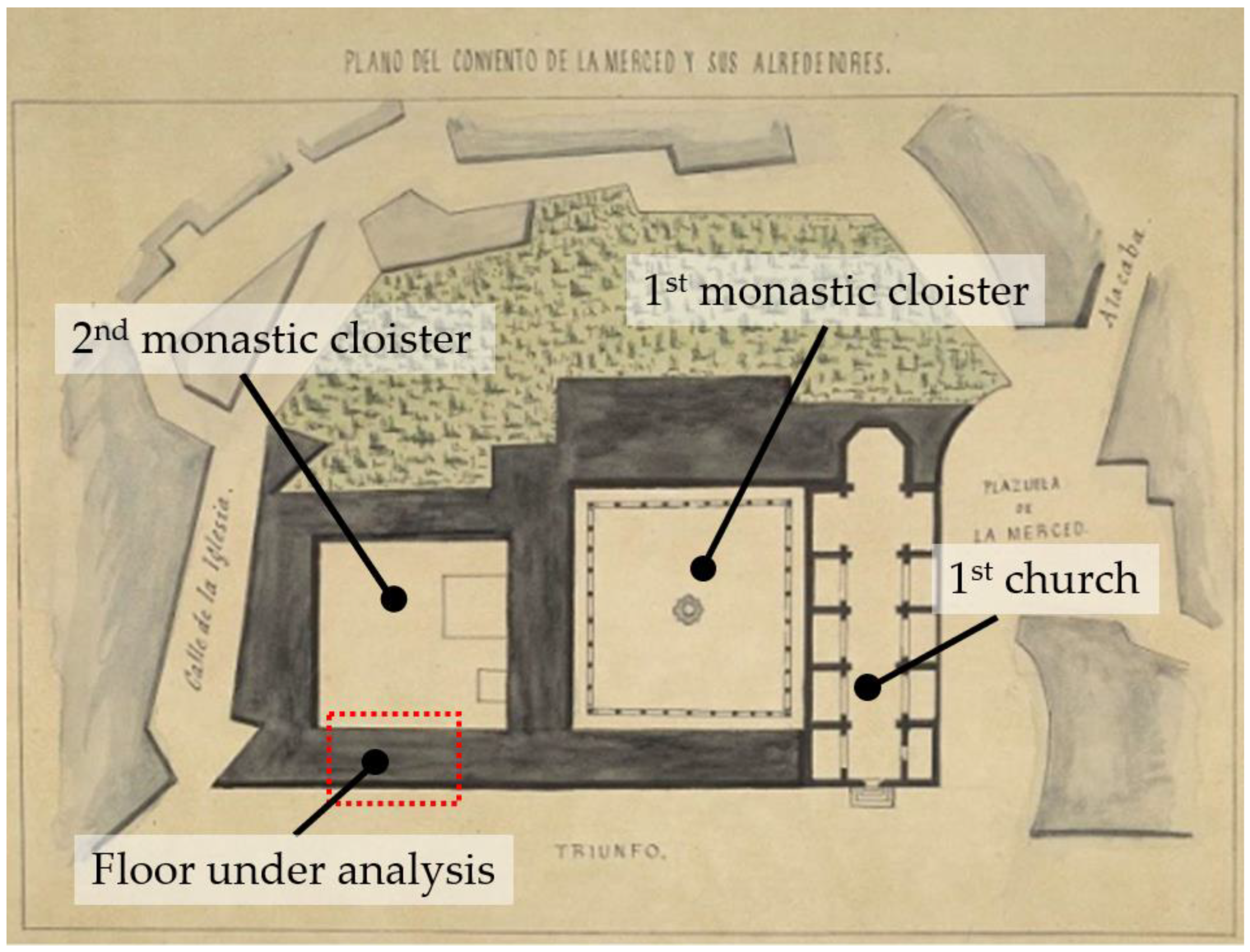
2.1. General Description of the Historical Building (Merced Convent)

In 1492, the Catholic Monarchs of Spain distributed among different ecclesiastical orders the land and houses left behind by exiles. One beneficiary was the Order of Mercy. In 1514, construction began in Granada of the church of La Merced, open and operative in 1530 (Figure 2). The building was designed in the shape of a Latin cross, with a mixture of late Gothic and Renaissance styles. Originally, the building had a set of Hispano-Muslim coffered ceilings, as well as a wood-paneled ceiling of enormous value, partly kept in storage in the famous monument the Alhambra. In 1639, the first monastic cloister with a square patio was inaugurated, whose central cloister features 36 arches in local marble. Between 1843 and 1846, the building had a uniquely military use, entailing extensive works in order to house up to 1000 soldiers. The wooden beams of the study floor that serve as an example of this work were included in this rehabilitation, along the western façade of the building (Figure 2). Since 12th July 1922, the National Monuments Commission has protected the building as a Site of Cultural Interest (BIC).

The floor of the study is located on the Convent’s first floor, and is made of local Sylvestris pine beams supported on lime-earth walls about 800 mm thick. The floor has 16 beams with an average section of 210 × 300 mm and an average length of 6800 mm, the average distance between axes being 77 mm (Figure 3). The beams were in the walls for around 200 mm without being embedded, thus constituting a bi-supported slab. The beams along their length presented variations in section. For this reason, five section measurement points were established, two at the beam heads (S1 and S5) and three more at L/4, L/2 and 3L/4, L being the total length of each element.

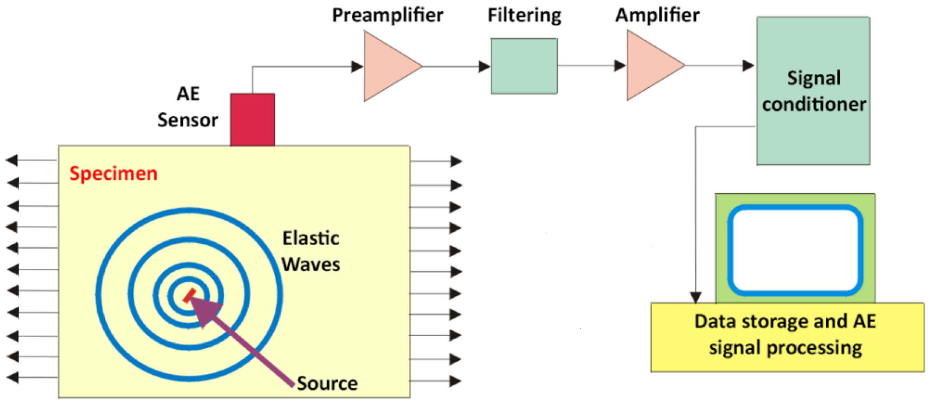
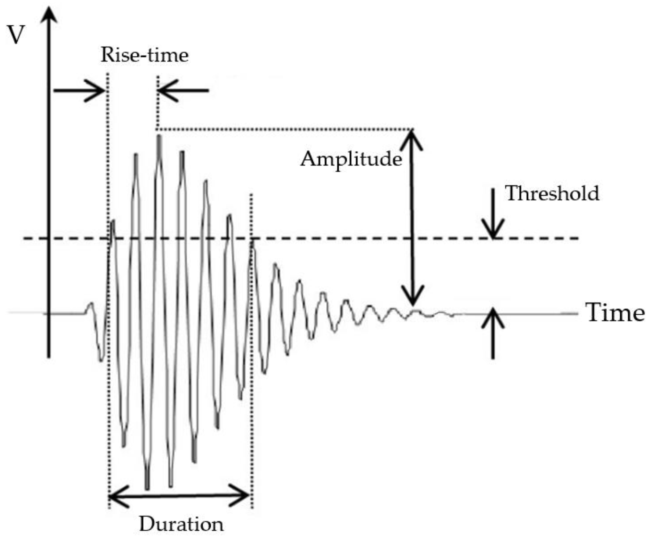
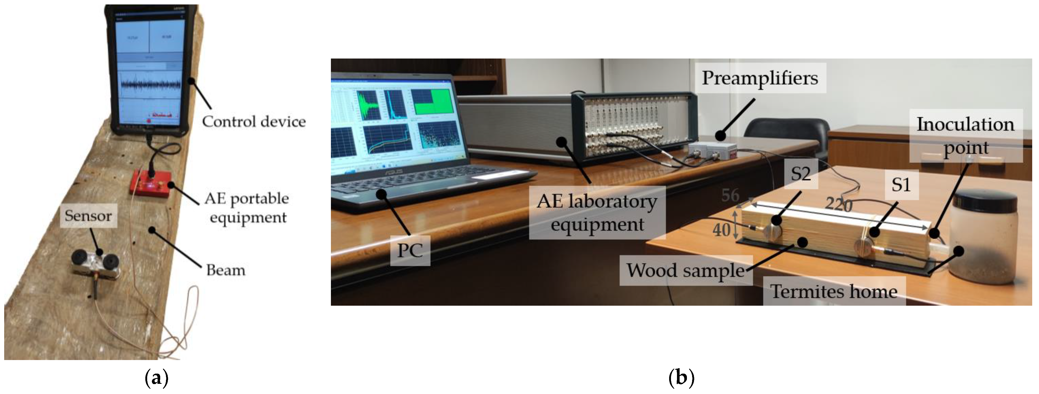
2.2. Acoustic Emission Analysis

Acoustic emission testing is an effective and passive NDT (non-destructive testing) method for monitoring the behavior of materials or structures when they are subjected to a change in the strain field. AE is the means by which energy is released, in the form of elastic waves within a material subjected to changes in the strain field produced by external actions. AE waves travel from the source through the structure and to its surface, where they can be detected by an AE sensor (piezoelectric sensor). The sensor can be mounted at some distance from the source, depending on the material attenuation (Figure 4). Thus, acoustic emission waves can be sourced by deformation processes, crack growth, dislocation movement, impact processes, friction, etc. A main advantage of AE testing, with respect to other NDT methods, is its ability to detect AE signals in real time as they are released from the materials themselves during the progress of the AE sources.

Transient acoustic emission signals can be generically characterized as shown in Figure 5. The traditional characteristics of these signals are the peak amplitude (A, dB) defined as the voltage of the transient, the duration (D, µs) defined by the time interval between the first and the last time the signal crosses the detection threshold, and the rise-time (RT, µs) defined as the interval of time between the first threshold crossing and the maximum amplitude. The threshold is a parameter defined by the user. It must be higher than the background electromagnetic noise existing in the place where the measurements are made.

In this paper, the acoustic emission method was applied to determine the active presence of xylophages in two different types of test: in situ tests carried out on the wooden beams of the floor, and laboratory tests with Reticulitermes termites artificially inoculated in wooden specimens.

The on-site inspection was carried out using single-channel portable equipment from Vallen Systeme^® (Wolfratshausen, Germany) for the acquisition of the acoustic emission signals. The sensors used were VS150H from Vallen Systeme^®, with a resonance frequency of around 150 kHz; they were placed on a base of silicone grease to ensure adequate transmission of acoustic waves between the wood and the sensor. In addition, a clamp was placed to ensure that the coupling remained stable during the test. After placing the sensor, the correct coupling was verified using a Nielsen HSU source (pencil lead break, PLB). A sampling frequency of 10 MHz and filtering in the band (70–300) kHz were established during the acquisition of the signals to avoid mechanical and electromagnetic environmental noise. Acoustic emission measurements were made at the ends of each beam and along every 30 cm of each beam. The photograph in Figure 6a depicts measurement on one of the beams.

For the tests carried out in the laboratory, Reticulitermes termites (Figure 7) were inoculated in a specimen of Sylvestris pine wood measuring 220 × 56 × 40 mm. The termites, specifically 200 workers and 8 soldiers, were stored in a plastic container. It had a small amount of moistened substrate, along with small pieces of wood from the same test tube as the food, to observe how the termites made their way through the connecting tube to the perforation provided in the specimen (Figure 6b). In the part closest to the edge of the specimen, the perforation was 2 cm long and 10 mm in diameter, followed by a second, narrower perforation 5 mm in diameter and 2 cm long.

The acoustic emission activity of termites was recorded continuously for 24 h after 83 days’ inoculation. During that time, to guarantee the survival of the termites, the test was carried out in a closed, ventilated room with little light, a constant temperature of 26 ± 2 °C and a relative humidity higher than 70 ± 5%. The acoustic emission activity in the laboratory tests was recorded by means of Vallen Systeme^® AMSY-6 equipment, as shown in Figure 6b, using VS150H sensors. A threshold of 30.1 dB, a sampling frequency of 5 MHz, preamplifiers with a gain of 34 dB and filters of (35, 800) kHz were chosen.

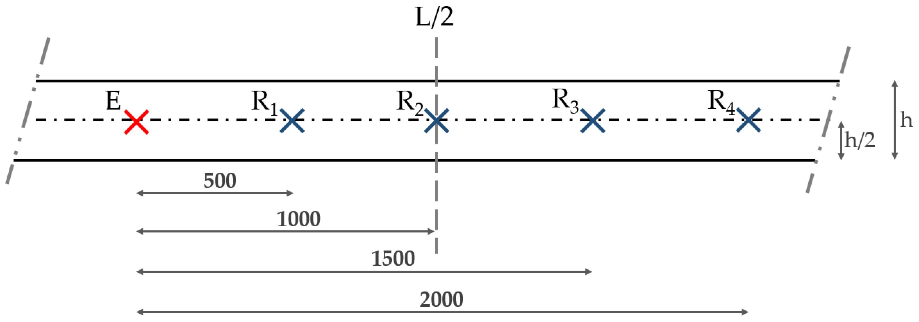
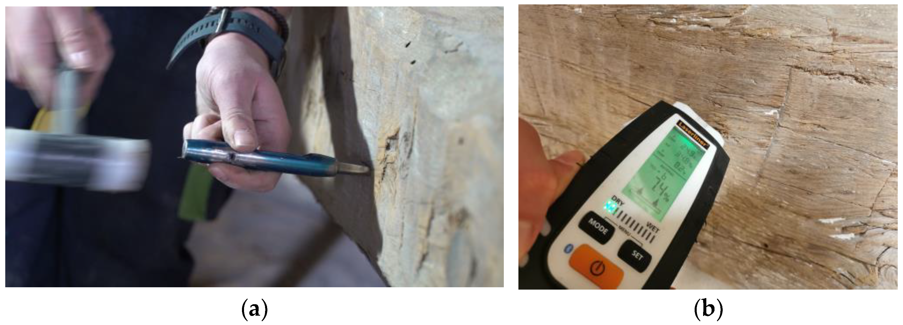
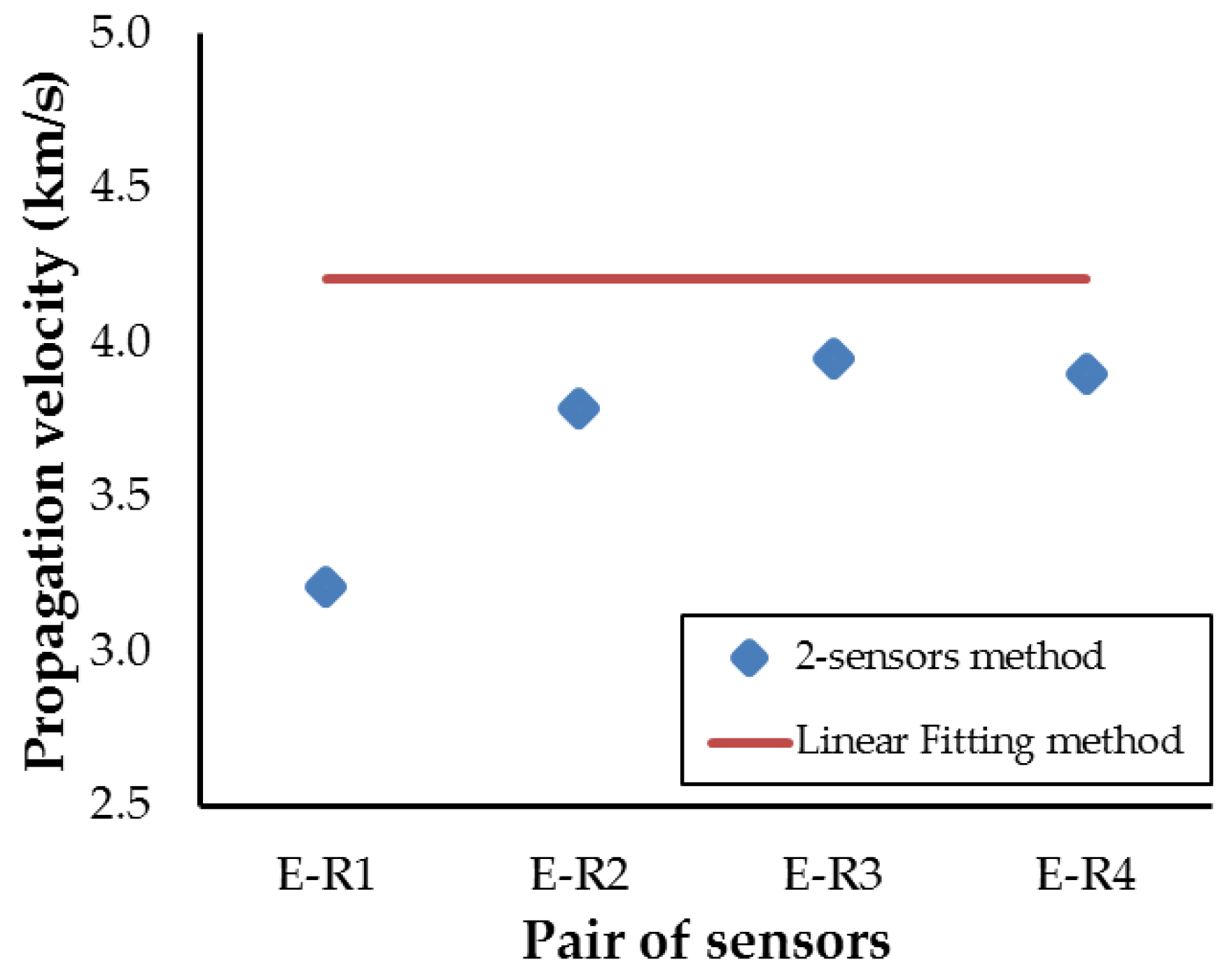
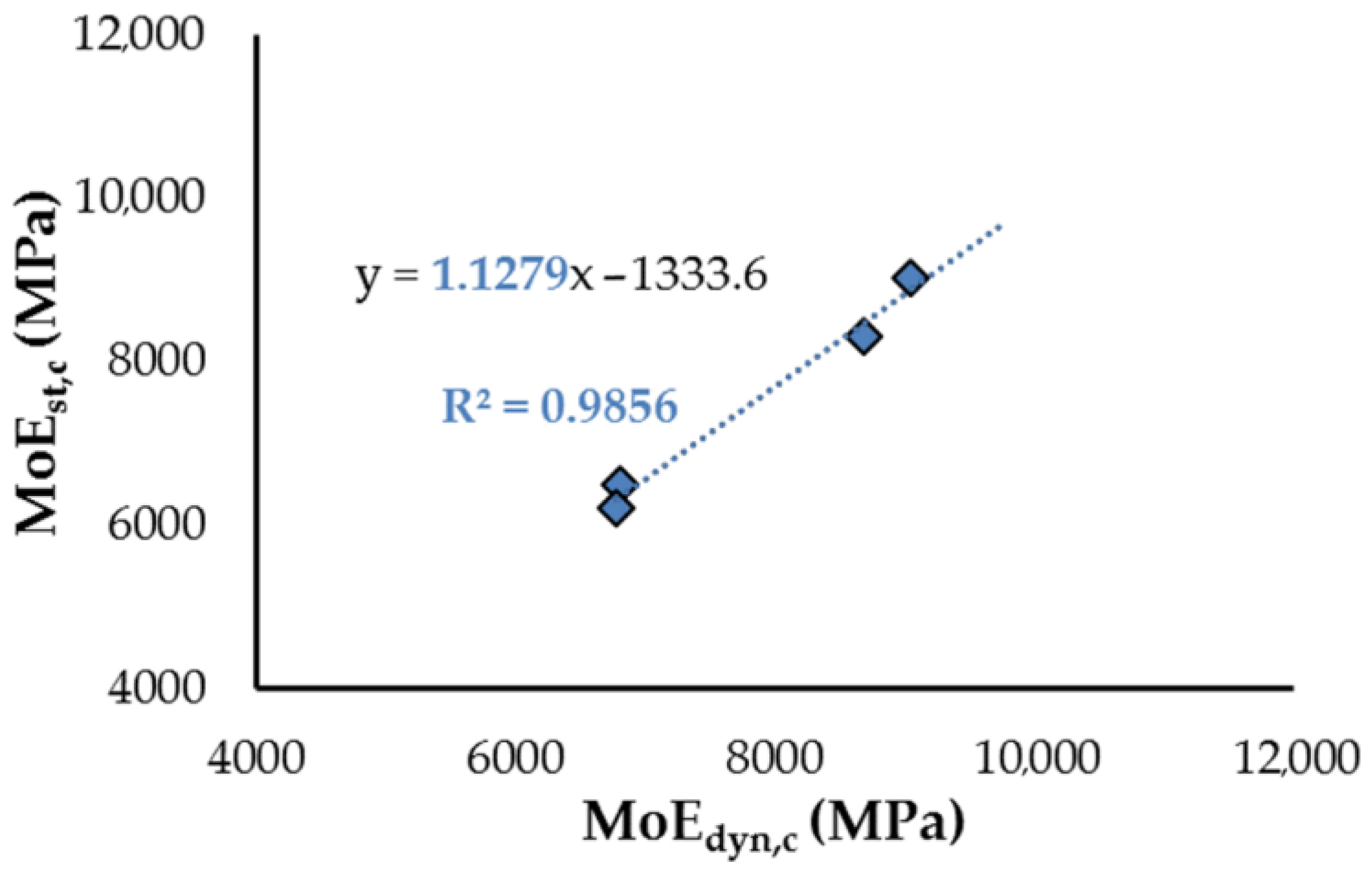
2.3. Elastic Wave Analysis

For each wooden beam of the floor, the dynamic modulus of elasticity (MoE_dyn) was obtained by means of the elastic wave technique. It was applied on a central area of the element, 200 mm long, in which the bending moment is maximum. Fakopp SD-02 sensors were driven into the wood with a pointed end in a 45° direction, in order to properly transmit the P mode of the elastic waves generated with an impact hammer weighing 100 g on the one of the sensors (Figure 8). To record the signals, a Picoscope^® oscilloscope (Saint Neots, UK) with a bandwidth of 20 MHz and a sampling frequency of 80 MS/s was used. The sensor tips were driven to a depth of 15 mm. Using a system of two separate sensors with a separation d, the time of flight of the elastic wave (ToF) was obtained (Δt = t₂ − t₁), where t₁ and t₂ are the arrival times of the wave to each sensor and c = d/Δt is the propagation velocity.

However, due to the heterogeneity of the wood and the presence of defects, the propagation velocity can vary considerably at different distances between sensors. To take this effect into account, a technique was applied by placing an impact sensor that acts as a wave emitter (E) and four receiving sensors (R_i; i: 1–4) spaced 500 mm apart, as depicted in Figure 8. In this way, the propagation velocity could be obtained as the slope of the regression line that best fits the relationship between the distance from sensors E and R_i (d_i) and the arrival times’ difference (Δt_i).

As expected, determining the arrival time of the signal is a critical aspect. Our previous work [33] showed that the Akaike method (AIC) introduces a significant improvement when it comes to obtaining the arrival time of a signal. This method acknowledges the fact that before the arrival of the wave, the recorded signal is purely electromagnetic noise with a high entropy. Yet, after the arrival of the wave, the entropy of the signal must be lower. Therefore, the arrival time can be obtained as the point at which the entropy difference of the time signal becomes its maximum, that is, when the Akaike function reaches the maximum value. This function is defined as:

AIC(k) = k · log (variance (x (1: k)) + N − k − 1) · log (variance (x (k + 1: N))

(1)

where N is the total number of signal data and k is the order of each signal sample, which varies from 1 to N. Thus, the arrival time at each sensor, t_i, is given by the time at which the absolute minimum of the AIC function is obtained.

When the propagation velocity of the elastic wave is known, c, an estimation of the dynamic elasticity modulus of each beam, can be obtained as [39]

MoE_dyn = ρ·c²

(2)

where ρ is the density of the beam. The density was obtained by extractions (micro-cores) carried out with a Trephor35 auger (Figure 9a). The sample was taken from areas of each beam away from knots, cracks and other pathologies. These micro-cores were 4 mm in diameter and 25 mm long. However, according to the EN 384:2016+A:2018 [40] standard, the MoE_dyn must be corrected to a reference relative moisture content of 12%. To do this, it is necessary to determine the actual relative moisture content of each beam when the elastic wave testing is carried out. This was measured by means of the HML701A hygrometer (Figure 9b) at five points on each beam to derive an average value. Accordingly, the corrected elastic modulus is given by:

MoE_dyn,c = MoE_dyn (1 + 0.01 (u − u_ref))

(3)

where u is the actual moisture content of the beam and u_ref is the reference moisture content (12%). Finally, once MoE_dyn,c and the density of each beam were known, its strength grade was assigned following the EN 384:2016+A:2018 [40].

For comparison reasons, the floor owner supplied only four of the 16 beams (beams numbered 1, 2, 14 and 15) when they were removed from the building. It was not possible to obtain more beams. These four beams were subjected to a mechanical four-point bending test in the elastic zone using a multi-testing machine (Figure 10). In this way, the elastic modulus, MoE_st, and its corrected value at 12% moisture content, MoE_st,c, were obtained.

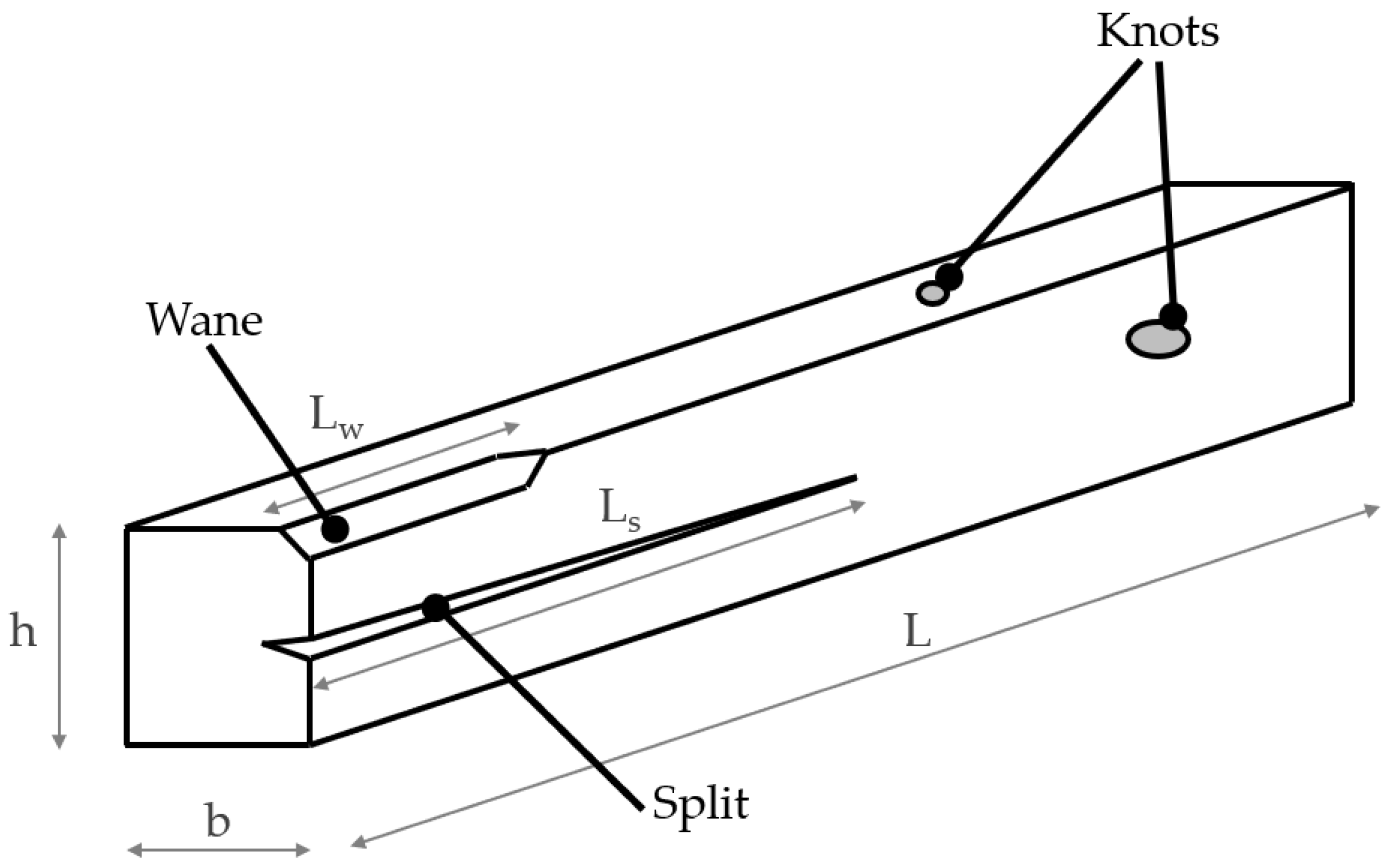
2.4. Visual Analysis

Visual analysis was carried out for each wooden beam to appraise its characteristics and pathologies. Once its density and moisture content were known, the dimensions of the element were measured in five sections to establish possible section losses, as explained in Section 2.1.

Assessment of decay of the material due to biotic attacks (Figure 11a) focused on the presence of galleries generated by xylophages and woodworms. It was not possible to visually determine whether the presence of these galleries owed to current or past activity. However, this analysis was correlated with the acoustic emission activity detected for each element, as described in Section 3.1.

In addition to the diagnosis of pathologies, a visual classification of each element was carried out following the Spanish standard UNE 56544:2022 [41] for coniferous wood, with the aim of assigning it a visual strength grading. The parameters measured were (Figure 12):

• Knots; these are singularities of the wood stemming from the presence of branches of the tree (Figure 11b). All knots were measured, including their diameter and their position on the beam. It was determined if they constituted through knots, edge knots or grouped knots.
• Splits; these are cracks in the radial and axial direction, occurring in wood when the resistance values are exceeded due to growth stresses or drying among other reasons (Figure 11c). Their length and position on the beam were determined. It was also determined whether they were non-passing splits, i.e., passing through the end or not through the end.
• Wanes; this defect appears in solid timber when, on one of its edges, part of the original curvature of the trunk is visible due to the absence of wood (Figure 11d). Wanes were classified according to their length and their relative dimension.

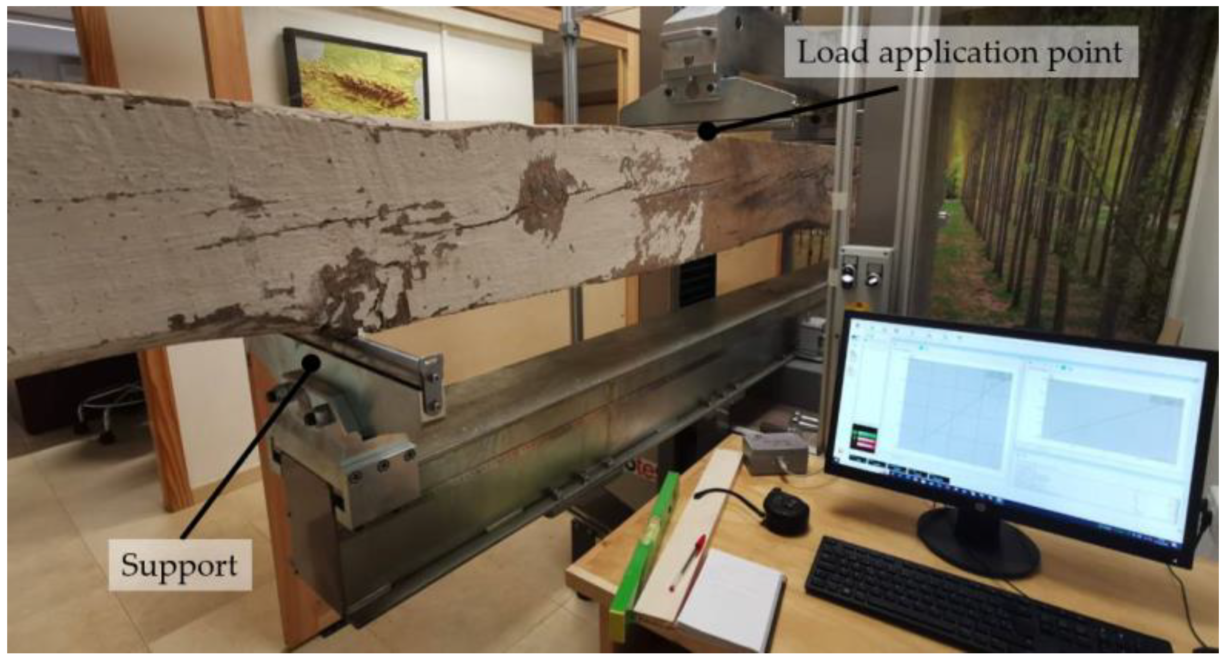
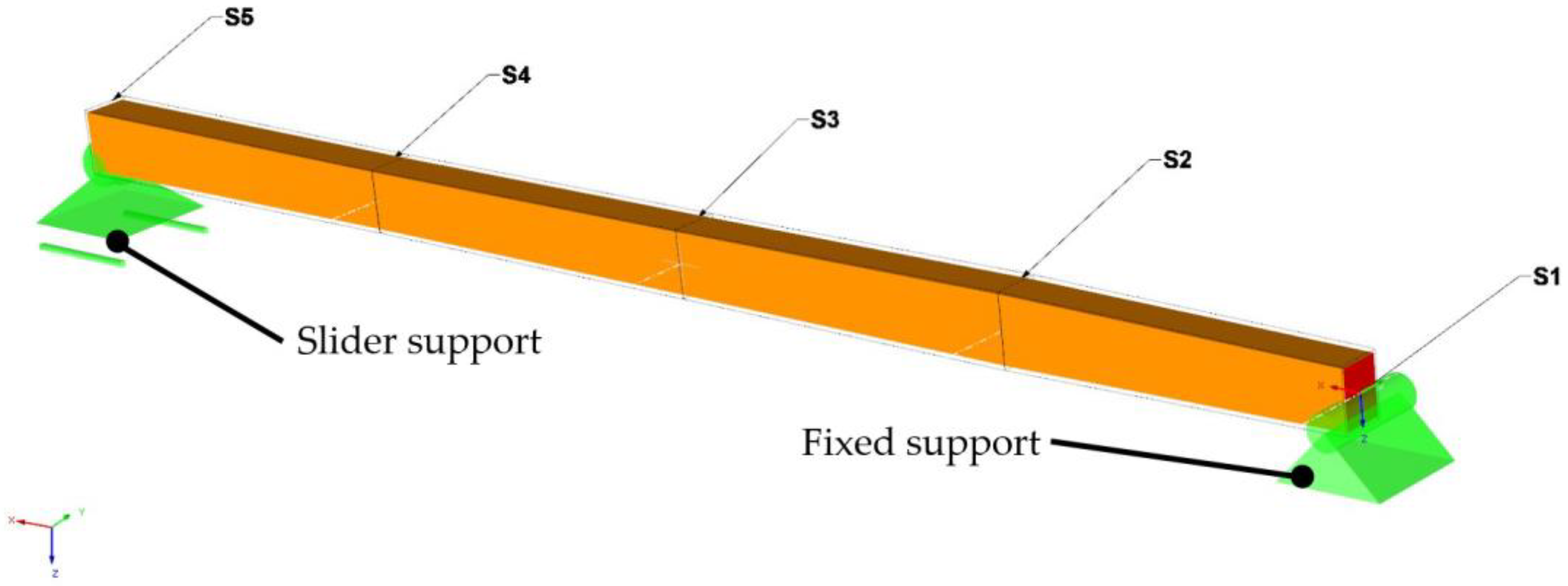
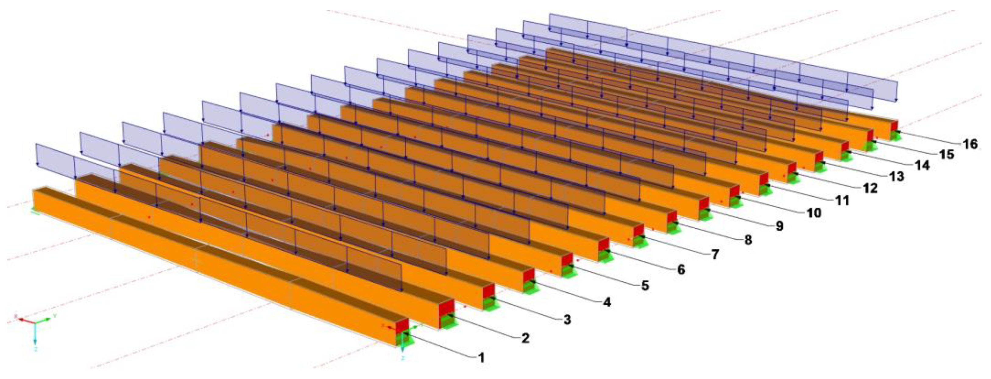
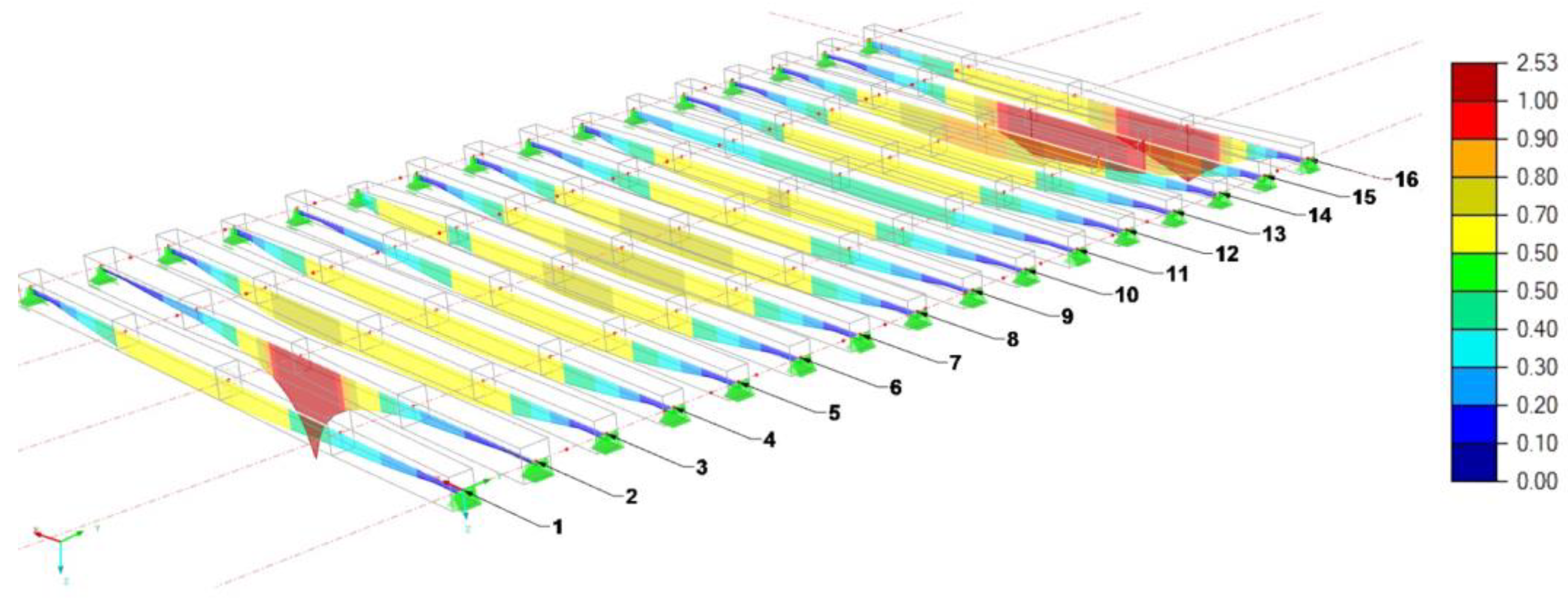
According to the thickness of the study piece (b) and all the characteristics examined, the visual strength class assigned could be MEG or Rejection. MEG is defined as structural wood of coarse squareness, and Rejection means that the element is not suitable for structural use. For Sylvestris pine, the visual strength class MEG corresponds to a strength class of C22.

2.5. Modelling

For each floor beam, numerical modelling was performed using Dlubal RFEM^® 5.27 software (Tiefenbach, Germany). Specifically, the RF-TIMBER-PRO module was used. As previously mentioned, the beams were considered to be bi-supported on the walls; that is, with a fixed support restricting 1 degree of freedom, and a slider restricting 2 degrees of freedom (Figure 13). The beams were three-dimensionally modelled as beam-type bar elements, meeting the criteria of being resistant to bending and capable of transmitting internal forces. The beams were divided into the five groupings, described in Section 2.1 (Figure 3).

For the finite element model, the Dlubal RFEM^® 5.27 software was used. With the model, the behavior of the 16-beam floor was evaluated. First, it was assumed that wood behaves as a linear isotropic material depending on boundary conditions and load configuration. The input parameters used for the constitutive model were the density and dynamic elastic modulus (MoE_dyn) of each element. These parameters were obtained by the elastic wave method described in Section 2.3. A Poisson’s ratio (ν) of 0.3 was used, and the shear modulus was calculated for each element according to the relationship G = MoE_dyn/(2(1 + ν)). The FEM model of each beam with a length of 6.8 m, is formed by 1D bar-type elements with a length of 1.70 m each. This allowed simulation of the variations in cross section that occurred in each structural element. In order to obtain accurate results with a reasonable computational cost, a convergence analysis of the results, based on the size of the elements, was carried out. An optimal mesh size of 100 mm was used, resulting in 68 elements per beam according to its length. This leads to 69 nodes per beam. Due to the fact that the object of the evaluation is of a general size, and to simplify the modelling, the presence of defects such as knots, cracks and resin pockets was not taken into account for a general analysis. According to the parameters introduced in the constitutive model, a strength class was assigned applying the EN 338:2016 standard [42] for timer. Likewise, the floor was assigned to service class 1 as an intermediate floor between habitable spaces included in the EN 1995-1-2:2014/AC:2009 [43]. The beams with an inter-axis around 77 mm were considered to work as a set and not individually; therefore, the coefficient k_sys = 1.1 was applied.

For the simulation, simple load cases were taken into account, including the following loads individually: (1) own weight of all the elements of the structure equal to 0.80 kN/m² (CC1); (2) overload of use expected (CC2), and given future office use, a value of 2.00 kN/m² was assigned; (3) occasional use overload (CC3), assigning a value of 2.00 kN. Figure 14 shows the numerical model of the wooden floor, with the distribution of loads distributed along each beam.

Subsequently, different load combinations were taken into account for different calculation states (

Table 1. Combinations of loads included in the numerical simulation.

Combination	Calculation State
	Ultimate limit state (ULS—fundamental)
CR1	γq CC1	Self weight
CR2	γG CC1 + γQ CC2	Self weight + live load
CR3	γG CC1/p + γQ CC3	Self weight + individual load
	Serviceability limit state (SLS)
CR4	kdef CC1/p + (1+ Ψ2 kdef) CC2	Characteristic/rare
CR5	CC2	Characteristic/quasi-permanent
CR6	(1+ kdef) CC1/p + Ψ2 (1+ kdef) CC2	Quasi-permanent
	Fire resistant (ULS—accidental)
CR7	CC1 + 0.50 CC2	Accidental—psi-1,1
CR8	CC1 + 0.50 CC3	Accidental—psi-1,2

): (1) ultimate limit state or depletion; (2) serviceability limit state; and (3) fire resistance. It is important to mention that the model did not include the remaining deflection, as well as the loss of section due to the wanes, the presence of cracks or knots or the loss of material caused by the presence of woodworm.

For analysis of the ULS, a safety increase coefficient of γ_G = 1.35 was applied for the permanent load or dead load. For the variable load or live load, γ_Q = 1.50 was used, combining the loads in three compositions (CR1, CR2 and CR3).

SLS was divided into three combinations: integrity of construction elements (CR5), comfort of users (CR6) and appearance of the work (CR7). For the calculation, the creep factor k_def = 0.6 was taken into account, in accordance with the provisions of the EN 1995-1-1:2004+A1 [44] standard for solid timber and service class 1. In addition, Ψ₂ = 0.3 was applied, which is a simultaneity coefficient for the quasi-permanent value of the use overload in correspondence with the administrative use of the premises established in the EN 1990:2002/A1:2005/AC:2010 standard [45].

Finally, verification of the fire resistance of the structural elements was analyzed. A resistance R = 60 min was assigned, according to their future administrative use. This calculation was made on the lateral and lower faces, considering that the upper face is protected from fire.

3. Results

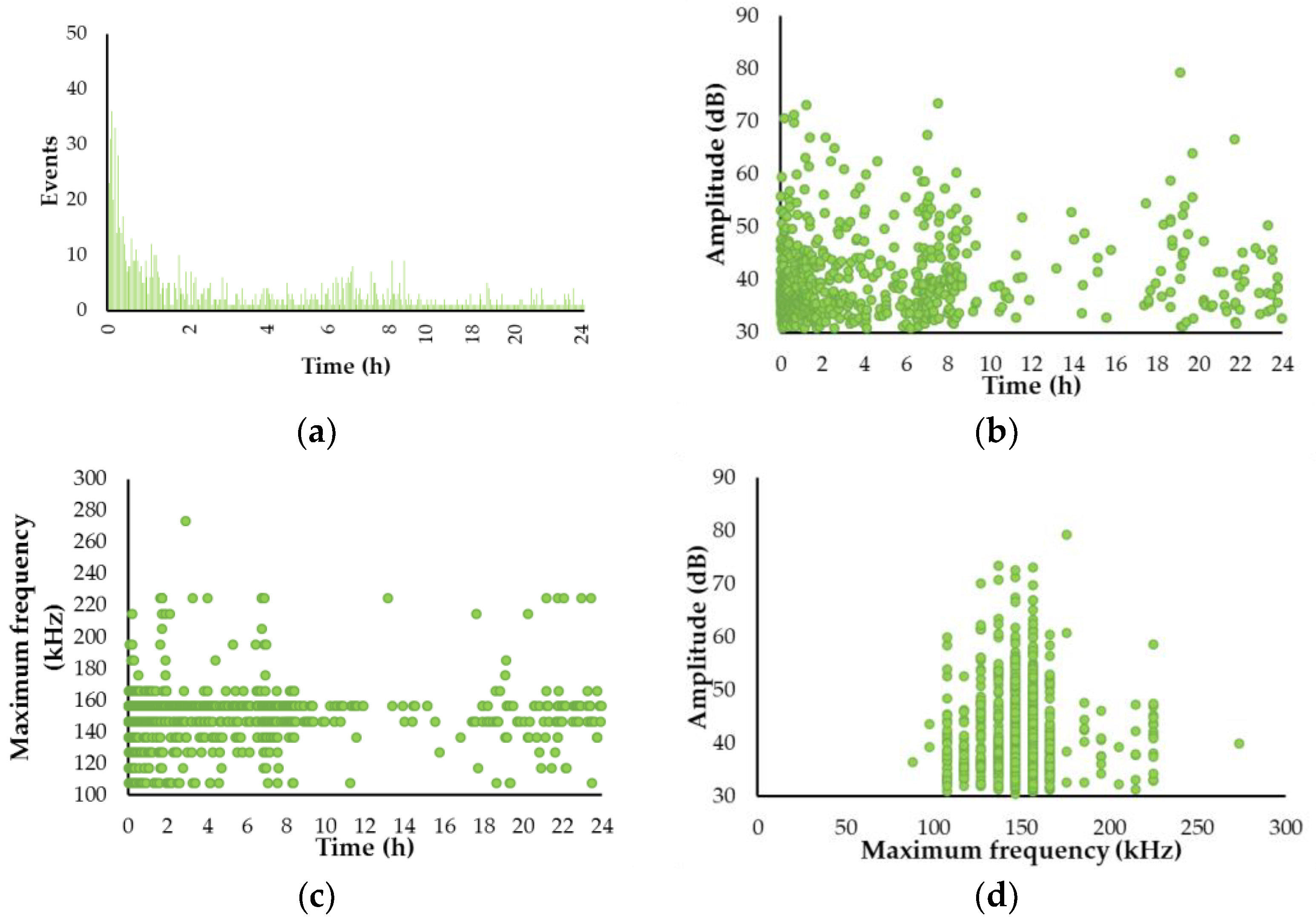
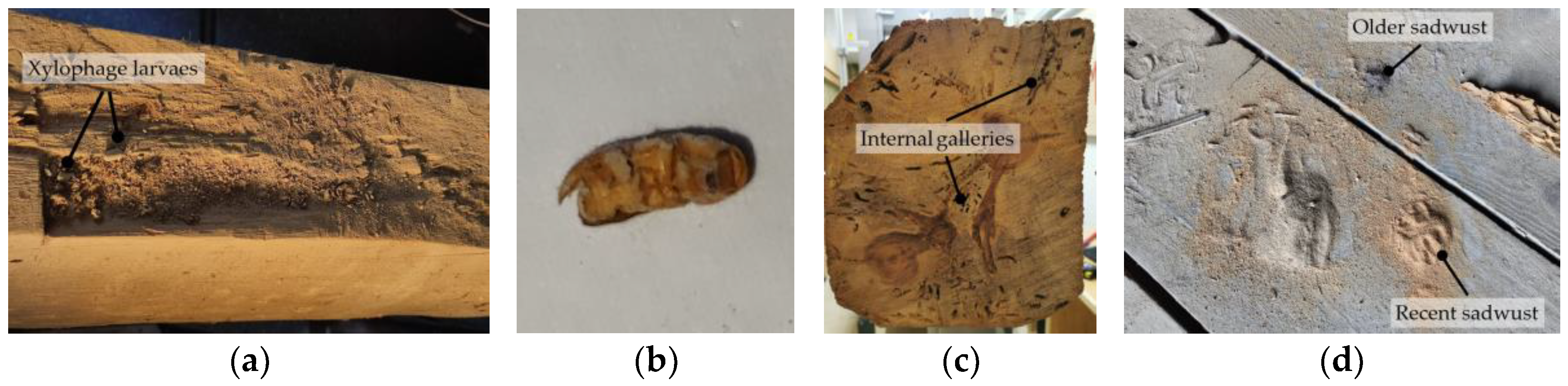
3.1. Detection of Active Xylophages by Means of the Acoustic Emission Method

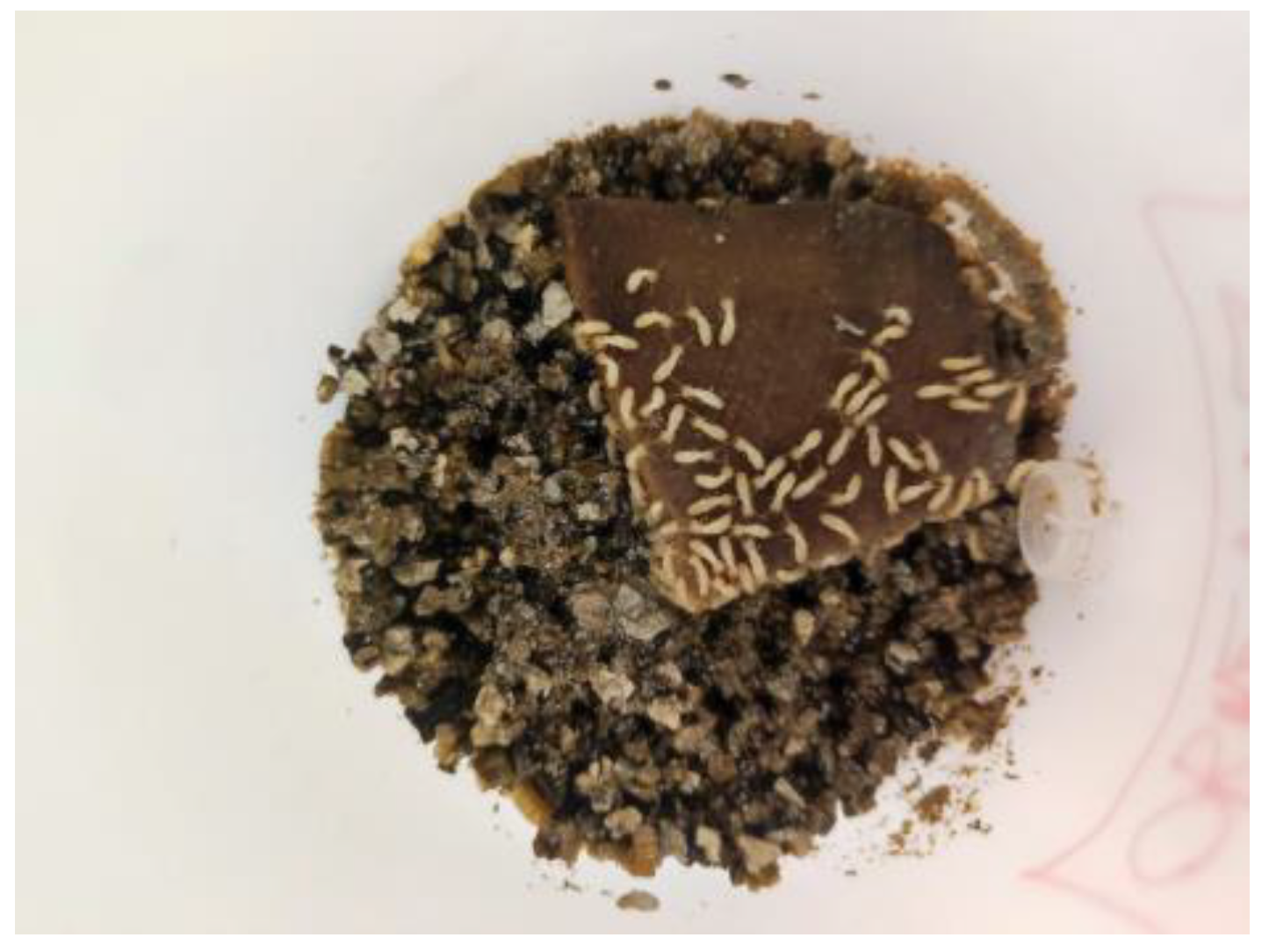
3.1.1. Laboratory Test with Inoculated Reticulitermes Termites

This section shows the results obtained during the test carried out for 24 h after 83 days from the inoculation of termites in a wood sample at the laboratory. A post-processing filter was applied to exclude signals coming from electromagnetic noise, which were previously characterized by D < 21 µs and RT < 5 µs. Figure 15 shows the plots of the number of events against time (a), the peak amplitude against time (b), the maximum frequency of the spectrum of each signal against time (c) and the maximum frequency of the spectrum against peak amplitude (d). Figure 16 shows an example of a recorded transient signal and its frequency spectrum within a time window of (−10, 140) µs.

3.1.2. AE Measured In Situ on the Wooden Floor

Acoustic emission activity associated with the active presence of xylophages was detected in six of the beams, as summarized in Section 3.3. The external deterioration of the beams associated with the presence of xylophages was evident, as can be seen in Figure 11a. After the detection of AE activity, an exhaustive visual inspection was carried out and the affected exterior wood was removed. During this inspection, xylophage larvae were found, as shown in Figure 17a,b. In addition, the appearance of light-colored sawdust was associated with recent galleries, as can be seen in Figure 17d, clearly demonstrating the reason behind the acoustic emission activity.

Figure 18 indicates the amplitude of the signals recorded during 10 s of testing in the six wooden beams with the active presence of xylophages. As an example, Figure 19 shows a particular acoustic emission signal recorded in beam 1 and its frequency spectrum, with the peak around the first resonance of the sensor (150 kHz), as expected.

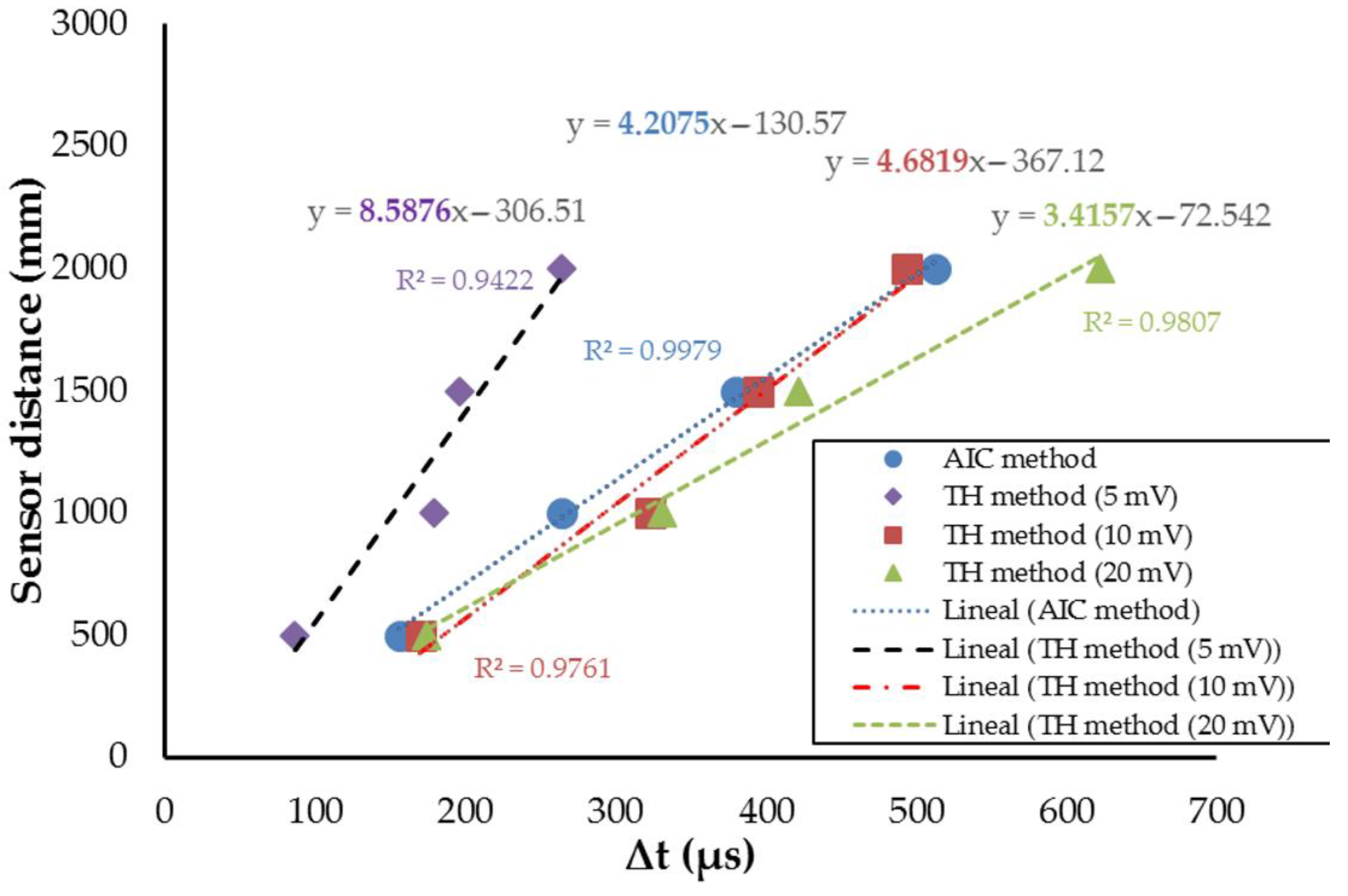
3.2. Acoustic Wave Analysis

Figure 20 shows the results obtained during the measurements of elastic waves carried out in beam 1 using the Akaike method (AIC) and the threshold method (TH) to determine the difference in arrival times between the sensor and the receiver, Δt. In the specific case of the threshold method, three different values were used: 5, 10 and 20 mV. The respective regression lines are shown. The slope is equal to the propagation velocity in km/s. The correlation coefficient (R²) using the Akaike method was 0.9979; meanwhile, when using the threshold method it, was lower, at 0.9422, 0.9761 and 0.9807, respectively. The propagation velocity obtained by means of the AIC technique was 4.20 km/s, while with the TH, the values were 8.58, 4.68 and 3.41 km/s, respectively, for 5, 10 and 20 mV. The variations for these velocities with respect to the one obtained with AIC amounted to 104%, 11% and −19%, respectively.

Alternatively, Figure 21 shows, for beam 1, the velocities obtained using the emitting sensor E and all the receiving sensors R_i (i: 1–4), by means of the arrival time obtained using the Akaike technique. The horizontal line represents the velocity obtained by the linear fitting. There are substantial differences between this average velocity and the individual ones, up to 31%.

Table 2. Non-destructive testing results and strength grading.

Beam	Velocity (km/s)	Density (kg/m3)	MoEdyn (MPa)	Moisture Content (%)	MoEdyn,c (MPa)	Strength Grading
1	4.21	531	9282	9.5	9050	C18
2	3.68	524	7005	9.3	6816	Rejection
3	4.10	516	8549	9.2	8309	C16
4	4.12	484	8066	8.9	7816	C14
5	4.29	444	8068	9.3	7850	C14
6	4.19	463	7999	8.8	7743	C14
7	3.89	599	8943	9.5	8719	C16
8	4.43	485	9360	8.7	9052	C18
9	4.54	496	10,096	8.9	9783	C20
10	3.93	554	8431	9.5	8220	C16
11	3.94	493	7556	9.2	7344	C14
12	4.67	446	9600	9.1	9321	C18
13	3.98	534	8347	9.0	8096	C16
14	4.12	536	8952	9.1	8692	C16
15	4.03	437	6995	9.0	6785	Rejection
16	3.90	498	7484	9.3	7282	C14

summarizes the results of the propagation velocity obtained with the AIC technique, along with density, dynamic elastic modulus, relative moisture content, moisture-corrected dynamic elastic modulus and strength grading, according to the UNE-EN 338 standard, for each of the 16 beams of the wooden floor.

Table 3. MoE_st,c and MoE_dyn,c comparison for the four beams tested to bending.

Beam	MoEst,c (MPa)	MoEdyn,c (MPa)
1	9015	9050
2	6494	6816
14	8300	8692
15	6208	6785

offers a comparison between the MoE_dyn,c and MoE_st,c for the four beams subjected to the bending test. Figure 22 shows the comparison between them and the regression line that fits the four points, resulting in a coefficient relation between the two MoEs of 1.12, with a correlation coefficient of R² = 0.98.

3.3. Visual Analysis

The results of the visual analysis performed on each beam are summarized in

Table 4. Summary of pathologies, and visual strength class according to UNE 56544:2022 [41], including the main cause of rejection for each beam.

Beam	Pathologies	Active Xylophages	Visual Grading	Main Cause of Rejection
1	Woodworm	Yes	Rejection	Wane
2	Reduced cross-section in beam center, woodworm, cracks, twist	Yes	Rejection	Wane
3	High humidity in beam head S1, woodworm, twist in beam head S1	Yes	Rejection	Wane
4	High humidity, woodworm, crack in tensile crack (1400–1700 mm), twist (0–2500 mm)	Yes	Rejection	Knot Wane
5	Woodworm, crack in tensile knot (1400 mm)		Rejection	Wane
6	Woodworm, high humidity in beam head S1, internal cavity, high reduced cross-section in beam head S5, deficient support in beam head S1 (170 mm)		Rejection	Knot Wane
7	Woodworm, crack in tensile crack (4900 mm)		Rejection	Knot Wane
8	Woodworm, twist in beam head S1 (0–2000 mm)		Rejection	Wane
9	Woodworm, crack in tensile knot (5000 mm), high presence of knots in beam center		Rejection	Wane
10	Woodworm, twist in beam head S1 (0–1850 mm), concentration of grouped knots in beam center (diameter = 110 mm)		Rejection	Wane
11	Woodworm, high deflection, reduced cross-section in end of beam	Yes	Rejection	Wane
12	Woodworm, twist in beam head S5		Rejection	Wane
13	Woodworm, twist in beam head S1, large knots in tensile part of beam center, reduced cross-section in beam head S5		Rejection	Wane
14	Woodworm, slight twist (1700–5000 mm)		Rejection	Wane
15	Woodworm		Rejection	Knot
16	Woodworm, twist	Yes	Rejection	Knot Wane

, including the most important pathologies detected, the presence of active xylophages with acoustic emission and the visual strength grading, indicating the main cause of rejection.

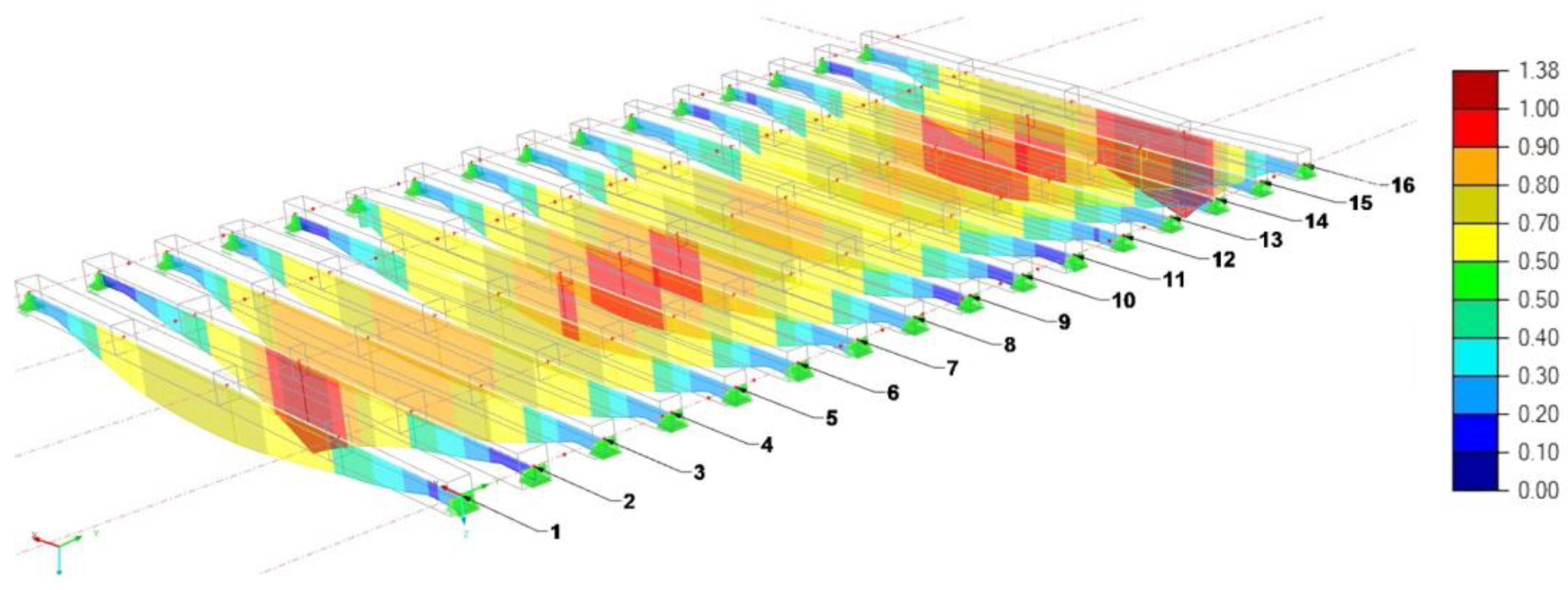
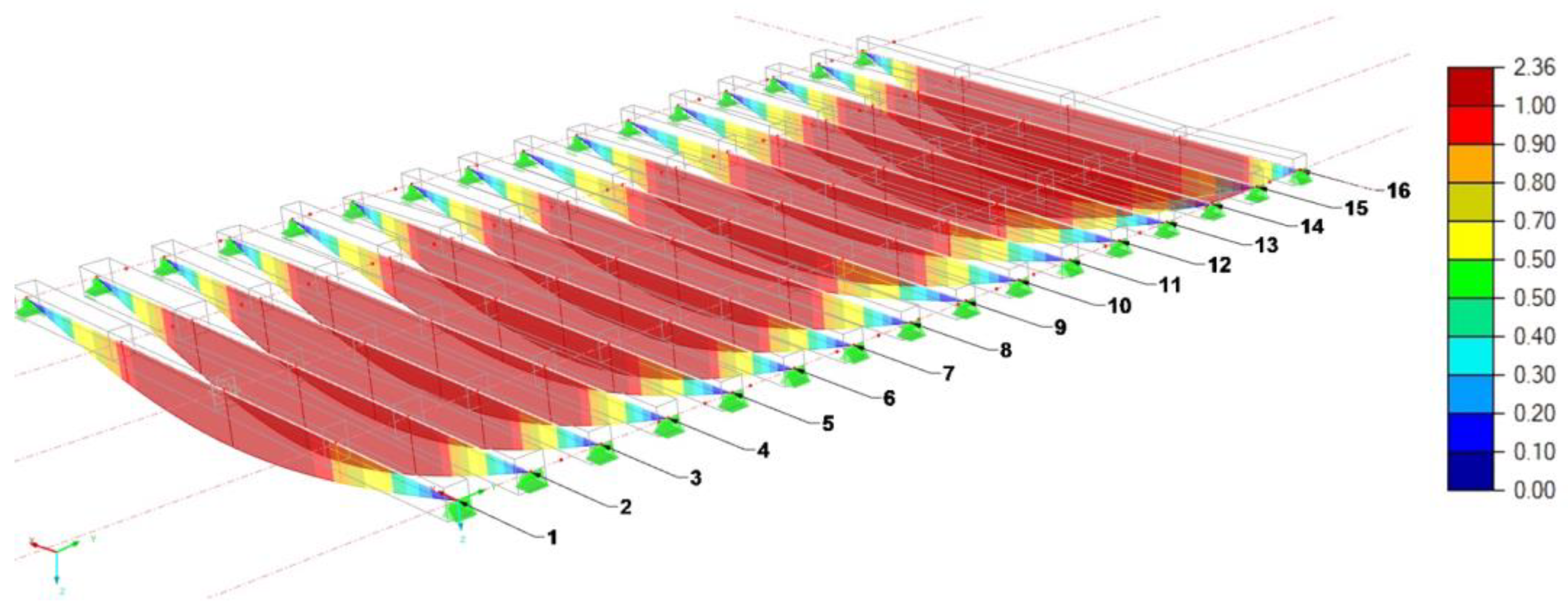
3.4. Numerical Analysis Results

Table 5. Summary of results for each combination and load situation. Cases of almost non-compliance with the minimum required (higher or equal to 90%) under the imposed loads are marked in orange.

Beam	ULS			SLS			Fire Resistance
				Integrity	Comfort	Appearance
	CR1	CR2	CR3	CR4	CR5	CR6	CR7	CR8
1	0.37	0.78	0.48	1.26	0.72	0.90	0.64	0.46
2	0.62	1.24	0.46	1.88	1.04	1.38	2.53	1.44
3	0.43	0.86	0.31	1.78	1.00	1.27	0.73	0.40
4	0.41	0.85	0.30	1.84	1.04	1.31	0.68	0.38
5	0.38	0.80	0.50	1.49	0.84	1.06	0.66	0.48
6	0.43	0.91	0.32	1.92	1.09	1.37	0.74	0.40
7	0.47	0.94	0.35	1.72	0.95	1.27	0.78	0.45
8	0.43	0.91	0.32	1.68	0.95	1.19	0.74	0.41
9	0.38	0.78	0.29	1.22	0.68	0.89	0.60	0.34
10	0.43	0.65	0.32	1.63	0.90	1.19	0.70	0.40
11	0.32	0.64	0.24	1.26	0.70	0.92	0.47	0.27
12	0.38	0.81	0.29	1.35	0.76	0.96	0.64	0.35
13	0.41	0.83	0.31	1.57	0.87	1.15	0.66	0.38
14	0.49	1.00	0.36	1.84	1.03	1.33	0.84	0.47
15	0.44	0.95	0.33	1.88	1.07	1.31	0.99	0.54
16	0.65	1.38	0.48	2.36	1.34	1.66	1.62	0.88

summarizes the numerical results obtained for each combination and load situation of every beam. If a beam reaches its maximum loading capacity, a value equal to 1 (100% exhaustion) is obtained. For example, beam 2 reached 62% of its maximum capacity (0.62) for combination CR1. However, it exceeded its carrying capacity by 24% (1.24) for the CR2 combination. It is observed that the CR4 combination is the most critical, beam 16 being the one with the worst result (an exhaustion of 236%). Figure 23, Figure 24 and Figure 25 show the envelope of the resulting diagrams for the different numerical analyses—specifically, for ULS (CR1, CR2 and CR3), SLS (CR4, CR5, and CR6) and fire resistance (CR7 and CR8). The value 1.0 represents 100% of the total capacity for each variable.

4. Discussion and Conclusions

The high acoustic emission activity of the termites discerned in the controlled laboratory test (Figure 15a) shows that these xylophages are fully detectable with sensors through their non-audible emissions, i.e., through resonant sensors at 150 kHz (Figure 15b). This means that in real situations, detection is possible without the interference of ambient audible noise below 20 kHz. In addition, it was seen that their emissions were up to 75 dB in amplitude. Most of the signals emitted were in the band between 100 and 250 kHz, owing to the resonance of the sensor (150 kHz). It was also deduced that the activity is not constant throughout the day, but changes over time, including periods of inactivity; this is of enormous importance in establishing inspection programs in real buildings using this technique.

In the acoustic emission measurements carried out on the wooden beams of the floor, activity was detected in just six of the 16 beams (1, 2, 3, 4, 11 and 16). According to Figure 19, however, the activity pattern was very different in beams 2, 3 and 4—in which the intensity is homogeneous and always below 40 dB—from that in beams 1, 11 and 16, wherein the activity comprises short periods of silence and a wide range of peak amplitudes, up to about 80 dB. The low amplitude of the activity recorded in beams 2, 3, 4 is most likely due to the fact that the attenuation of the acoustic emission signal can vary considerably from one beam to the next, given their different levels of internal deterioration linked to the existence of galleries associated with xylophage activity. Moreover, in view of Table 4, which indicates that all the beams had visible cavities due to xylophages, it is noteworthy that activity was detected in only six beams. The rest probably no longer had active xylophages, but had in the past. The existing xylophages were possibly woodworms, as, when cutting the beams, some dead larvae were discovered.

From the results of the non-destructive testing of elastic waves, it follows that the Akaike technique is much more stable than the threshold technique for detecting arrival time. The latter technique is highly sensitive to the chosen threshold, which is not known a priori. Likewise, it is shown that (Figure 21) the heterogeneity of the wood makes it impossible to obtain a stable value for propagation speed throughout the beam; rather, it depends on the inspected area and the emitter–sensor distance. For this reason, it is advisable to make measurements at several points and obtain the average velocity through a regression analysis of the difference between the distance and the arrival times.

Regarding the four beams that underwent bending tests in the laboratory, a very good concordance between the dynamic elastic modulus and the static elastic modulus was obtained. A correlation coefficient of 0.986 was derived, though because of the low number of samples, this value is not statistically significant. Still, this good correlation partly validates the experimental results in the field and in the laboratory.

Table 6. Summary of characteristics considered in non-destructive testing multi-analysis. ULS, SLS and Fire resistant indicate the % of load capacity exhausted. A percentage of 90 was established as the admissibility threshold for the ULS, SLS and Fire resistance features. Non-rejection strength class was established as the admissibility threshold for strength grading, both in visual and elastic wave methods.

Beam	Visual Grading	Elastic Waves Grading	ULS (%)	SLS (%)	Fire Resistant (%)
1	Rejection	C18		>90
2	Rejection	Rejection	>90	>90	>90
3	Rejection	C16		>90
4	Rejection	C14		>90
5	Rejection	C14		>90
6	Rejection	C14	>90	>90
7	Rejection	C16	>90	>90
8	Rejection	C18	>90	>90
9	Rejection	C20		>90
10	Rejection	C16		>90
11	Rejection	C14		>90
12	Rejection	C18		>90
13	Rejection	C16		>90
14	Rejection	C16	>90	>90	>90
15	Rejection	Rejection	>90	>90	>90
16	Rejection	C14	>90	>90

shows a summary of the results obtained through non-destructive testing techniques (visual, elastic waves and numerical simulation). Five features were established in this multi-analysis: visual strength class, elastic wave strength class, bearing capacity in ULS, the SLS and fire resistance.

Due to their multiple defects, being very old sawn wood beams without any type of prior selection or grading at the sawmill, all the beams give a visual strength class of rejection. In addition, most likely owing to high deterioration by xylophages, the dynamic elastic modulus of the beams did not exceed 9700 MPa (this value is corroborated by the four flexural tests carried out), which provides a low strength class for this species (most beams are below or equal to C18). However, the number of rejections determined by the elastic wave method was much lower than that determined by visual inspection, as there were only two rejected beams (2 and 15). This finding demonstrates that visual analysis clearly underestimates the strength grading, mainly because the defects (which visually determine the strength grading) mainly affect the maximum stress (modulus of rupture). In addition, the visual classification does not take into account the position of the knots along the element in bending. This is of vital importance, as a knot in compression and close to the supports is practically harmless to the resistance capacity. However, a knot with a smaller diameter located in the zone of greater moment and tension can have a significant influence on the bearing capacity of the element.

In turn, it is seen that all the beams exceeded the limit of 0.9 for SLS, that is, the current deflection restrictions for integrity, safety, comfort and appearance. This is because these beams were put in place without any legislative framework or restrictions, which are currently key for structural design. Meanwhile, seven beams exceeded the limit of 0.9 for SLS. The main reasons for non-compliance would be the substantial variations in the sections throughout the piece and the presence of wanes, together with the low modulus of elasticity. Finally, three beams exceeded the limit of 0.9 for resistance to fire, coinciding with the beams whose section reduction was most pronounced and therefore not meeting the section margins necessary to comply with resistance R60.

As can be seen, only two beams did not comply with the all five analyzed features—beams 2 and 15, which gave very low elastic modulus values below 7000 MPa.

Having obtained the analysis features, attention turned to determining which beams should be replaced by new ones, repaired or reinforced or simply kept without intervention. To this end, the results of this study and the intrinsic heterogeneity of wood as a natural material underline that decision making, involving such an economic and heritage impact, cannot be based on a single feature. On the contrary, it is proposed that criteria should be adopted based on several features (hence the multi-feature analysis). It is necessary to establish categories or groups of deterioration levels and then establish the decision-making criteria.

For the analyzed floor,

Table 7. Rejected beams as a function of the number of non-passing features considered for rejection.

Number of Non-Passing Features Considered for Rejection	Rejected Beams	Number of Rejected Beams
≥1	1–16	16
≥2	1–16	16
≥3	2, 6–8, 14–16	7
≥4	2, 15–16	3
≥5	2, 15	2

presents a first approach to the problem based on establishing a number of features that must not exceed the established admissibility thresholds for the structural element to be considered rejected (and therefore for repair or replacement). The most restrictive case would be to consider that when one of the five variables considered does not meet the established admissibility thresholds, the beam would be automatically rejected. In this case, all 16 beams would be rejected. Similarly, if elimination is decided when at least two features do not meet the established admissibility thresholds, all 16 beams would likewise be rejected. Yet, if three features are required for rejection, only seven beams would be eliminated. The most permissive case would be to eliminate the beam only if the five characteristics are not met. In this case, just two beams would be rejected.

In the particular case of the floor of the Merced Convent, the owner of the building and the engineering office decided to establish as a substitution criterion that at least two characteristics did not meet the established admissibility thresholds. Consequently, all 16 beams were replaced.

An alternative means of proceeding with a multi-feature analysis is that represented in

Table 8. Categories of damaged beams depending of the number of non-passing features. With * are the beams at which acoustic emission associated with active xylophages was detected.

Category	Number of Non-Passing Features	Beams
5	5	2*, 15
4	4	16*
3	3	6, 7, 8, 14
2	2	1*, 3*, 4*, 5, 9, 10, 11*, 12, 13
1	1	-
0	0	-

. It establishes up to six categories for beams, according to the number of characteristics not meeting the required admissibility threshold values. Under this classification, individual decisions can be made for each beam according to the category it pertains to. Here, the owner of the Merced Convent structure and the engineering office decided to replace all the beams that were in category 2 or higher categories, that is, all 16 beams of the floor. In Table 8, the beams in which acoustic emission detected active xylophages are also marked for practical reasons; the infected element requires treatment for xylophage elimination, and a prevention and surveillance protocol is required for the rest of the elements, given the high power of infection extending to nearby elements.

Consequently, it can be concluded that the non-destructive inspection of old wooden structures—conditioned by a high variety of wood, the existence of many natural defects, and the loss of rigidity due to decay and cavities produced by xylophages—through visual, acoustic and numerical methods can be a very powerful tool. The perspective of multi-feature analysis for decision making, aided by artificial intelligence, provides sound criteria and thresholds of acceptance and categorization to be considered by the owner of the structure and the engineering office. In order to obtain a behavior closer to reality, in future works, 3D-FEM modelling will be carried out, introducing the natural defects of wood into the model.

References

1. Faherty, K.F.; Williamson, T.G. Wood Engineering and Construction. Handbook; McGraw-Hill: Oxford, UK, 1998. [Google Scholar]
2. Palma, P.; Steiger, R. Structural health monitoring of timber structures—Review of available methods and case studies. Constr. Build. Mater. 2020, 248, 118528. [Google Scholar] [CrossRef]
3. Ghaly, A.; Edwards, S. Termite damage to buildings: Nature of attacks and preventive construction methods. Am. J. Eng. Appl. Sci. 2011, 4, 187–200. [Google Scholar] [CrossRef]
4. Llana, D.F.; Iñiguez-Gonzalez, G.; Díez, M.R.; Arriaga, F. Nondestructive testing used on timber in Spain: A literature review. Maderas-Cienc. Tecnol. 2020, 22, 133–156. [Google Scholar] [CrossRef] [Green Version]
5. French, J.R.J.; Ahmed, B.M.; Thorpe, J. Deciding the age of subterranean termite damage in buildings. In Proceedings of the 41st Annual International Research Group of Wood Protection Conference, Biarritz, France, 9–13 May 2010. [Google Scholar]
6. Ahmed, B.M.; French, J.R.J. An overview of termite control methods in Australia and their link to aspects of termite biology and ecology. Pak. Entomol. 2008, 30, 101–118. [Google Scholar]
7. Cavaleri, T.; Pelosi, C.; Ricci, M.; Laureti, S.; Romano, F.P.; Caliri, C.; Ventura, B.; De Blasi, S.; Gargano, M. IR Reflectography, Pulse-Compression Thermography, MA-XRF, and Radiography: A Full-Thickness Study of a 16th-Century Panel Painting Copy of Raphael. J. Imaging 2022, 8, 150. [Google Scholar] [CrossRef]
8. Laureti, S.; Colantonio, C.; Burrascano, P.; Melis, M.; Calabrò, G.; Malekmohammadi, H.; Sfarra, S.; Ricci, M.; Pelosi, C. Development of integrated innovative techniques for paintings examination: The case studies of The Resurrection of Christ attributed to Andrea Mantegna and the Crucifixion of Viterbo attributed to Michelangelo’s workshop. J. Cult. Herit. 2019, 40, 1–16. [Google Scholar] [CrossRef]
9. Tavakolian, P.; Shokouhi, E.B.; Sfarra, S.; Gargiulo, G.; Mandelis, A. Non-destructive imaging of ancient marquetries using active thermography and photothermal coherence tomography. J. Cult. Herit. 2020, 46, 159–164. [Google Scholar] [CrossRef]
10. Gavrilov, D.; Maev, R.G.; Almond, D.P. A review of imaging methods in analysis of works of art: Thermographic imaging method in art analysis. Can. J. Phys. 2014, 92, 341–364. [Google Scholar] [CrossRef]
11. Fiocco, G.; Ceccarelli, S.; Albano, M.; Rovetta, T.; Malagodi, M.; Orazi, N.; Paoloni, S. Structural feature investigation of wooden artifacts through imaging techniques: A step forward in the preservation of historical musical instruments. J. Phys. Conf. Ser. 2022, 2204, 012033. [Google Scholar] [CrossRef]
12. Grosse, C.U.; Ohtsu, M. Acoustic Emission Testing; Springer: Berlin, Germany, 2008. [Google Scholar]
13. Mizutani, Y. Practical Acoustic Emission Testing; Springer: Tokyo, Japan, 2016. [Google Scholar]
14. Ono, K. Application of acoustic emission for structure diagnosis. Diagnostyka 2011, 2, 3–18. [Google Scholar]
15. Martínez-Jequier, J.; Gallego, A.; Suarez, E.; Juanes, F.J.; Valea, A. Real-time damage mechanisms assessment in CFRP samples via acoustic emission Lamb wave modal analysis. Compos. Pt. B-Eng. 2015, 68, 317–326. [Google Scholar] [CrossRef]
16. Rescalvo, F.J.; Valverde-Palacios, I.; Suarez, E.; Roldán, A.; Gallego, A. Monitoring of carbon fiber-reinforced old timber beams via strain and multiresonant acoustic emission sensors. Sensors 2018, 18, 1224. [Google Scholar] [CrossRef] [PubMed]
17. Sagasta, F.; Zitto, M.E.; Piotrkowski, R.; Benavent-Climent, A.; Suarez, E.; Gallego, A. Acoustic emission energy b-value for local damage evaluation in reinforced concrete structures subjected to seismic loadings. Mech. Syst. Signal Process. 2018, 102, 262–277. [Google Scholar] [CrossRef]
18. Rescalvo, F.J.; Aguilar-Aguilera, A.; Suarez, E.; Valverde-Palacios, I.; Gallego, A. Acoustic emission during wood-CFRP adhesion tests. Int. J. Adhes. Adhes. 2018, 87, 79–90. [Google Scholar] [CrossRef]
19. Gallego, A.; Benavent-Climent, A.; Suarez, E. Concrete-Galvanized Steel Pull-Out Bond Assessed by Acoustic Emission. J. Mater. Civ. Eng. 2015, 28, 04015109. [Google Scholar] [CrossRef]
20. Nasir, V.; Ayanleye, S.; Kazemirad, S.; Sassani, F.; Adamopoulos, S. Acoustic emission monitoring of wood materials and timber structures: A critical review. Constr. Build. Mater. 2022, 350, 128877. [Google Scholar] [CrossRef]
21. Fujii, Y.; Noguchi, M.; Imamura, Y.; Tokoro, M. Using acoustic emission monitoring to detect termite activity in wood. For. Prod. J. 1990, 40, 34–36. [Google Scholar]
22. Gonzalez de la Rosa, J.J.; Puntonet, C.G.; Lloret, I. An application of the independent component analysis to monitor acoustic emission signals generated by termite activity in wood. Measurement 2005, 7, 63–76. [Google Scholar] [CrossRef]
23. Robbins, W.P.; Mueller, R.K.; Schaal, T.; Ebeling, T. Characteristics of acoustic emission signals generated by termite activity in wood. In Proceedings of the IEEE 1991 Ultrasonics Symposium, Orlando, FL, USA, 9–11 December 1991; pp. 1047–1051. [Google Scholar]
24. Indrayani, Y. Feeding activities of the dry-wood termite Cryptotermes domesticus (Haviland) under various relative humidity and temperature conditions using acoustic emission monitoring. Jpn. J. Environ. Entomol. Zool. 2003, 14, 205–212. [Google Scholar]
25. Indrayani, Y.; Yoshimura, T.; Yanase, Y.; Fujii, Y.; Imamura, Y. Evaluation of the temperature and relative humidity preferences of the western dry-wood termite Incisitermes minor (Hagen) using acoustic emission (AE) monitoring. J. Wood Sci. 2007, 53, 76–79. [Google Scholar] [CrossRef]
26. González de la Rosa, J.J.; Lloret, I.; Moreno, A.; Puntonet, C.G.; Górriz, J.M. Wavelets and wavelet packets applied to detect and characterize transient alarm signals from termites. Measurement 2006, 39, 553–564. [Google Scholar] [CrossRef]
27. González de la Rosa, J.J.; Agüera Pérez, A.; Palomares Salas, J.C.; Sierra Fernández, J.M. A novel measurement method for transient detection based in wavelets entropy and the spectral kurtosis: An application to vibrations and acoustic emission signals from termite activity. Measurement 2015, 68, 58–69. [Google Scholar] [CrossRef]
28. Oliver-Villanueva, J.; Abian-Perez, M. Advanced wireless sensors for termite detection in wood constructions. Wood Sci. Technol. 2013, 47, 269–280. [Google Scholar] [CrossRef]
29. Xue, S.; Zhou, H.; Liu, X.; Wang, W. Prediction of compression strength of wood usually used in ancient timber buildings by using resistograph and screw withdrawal tests. Wood Res. 2019, 64, 249–260. [Google Scholar]
30. Franco, D.; Nunes, L.; Saporiti, J.; Brito, J. Timber in buildings: Estimation of some properties using Pilodyn® and Resistograph®. In Proceedings of the 12th International Conference on Durability of Building Materials and Components, Porto, Portugal, 12–15 April 2011. [Google Scholar]
31. Lenzen, F.; Kim, K.I.; Schäfer, H.; Nair, R.; Meister, S.; Becker, F.; Garbe, C.S.; Theobalt, C. Denoising Strategies for Time-of-Flight Data. In Time-of-Flight and Depth Imaging. Sensors, Algorithms, and Applications; Springer: Berlin, Germany, 2013; pp. 25–45. [Google Scholar]
32. Chauhan, S.; Sethy, A. Differences in dynamic modulus of elasticity determined by three vibration methods and their relationship with static modulus of elasticity. Maderas Cienc. Tecnol. 2016, 18, 373–382. [Google Scholar] [CrossRef]
33. Rescalvo, F.J.; Ripoll, M.A.; Suarez, E.; Gallego, A. Effect of location, clone, and measurement season on the propagation velocity of poplar trees using the Akaike information criterion for arrival time determination. Materials 2019, 12, 356. [Google Scholar] [CrossRef] [Green Version]
34. Li, X.; Shang, X.; Morales-Esteban, A.; Wang, Z. Identifying P phase arrival of weak events: The Akaike Information Criterion picking application based on the Empirical Mode Decomposition. Comput. Geosci. 2017, 100, 57–66. [Google Scholar] [CrossRef]
35. Mborah, C.; Ge, M. Enhancing manual P-phase arrival detection and automatic onset time picking in a noisy microseismic data in underground mines. Int. J. Min. Sci. Technol. 2018, 28, 691–699. [Google Scholar] [CrossRef]
36. Kolassa, S. Combining exponential smoothing forecasts using Akaike weights. Int. J. Forecast. 2011, 27, 238–251. [Google Scholar] [CrossRef]
37. Fonseca, C.; D’Ayala, D.; Fernandez Cabo, J.L.; Díez, R. Numerical modelling of historic vaulted timber structures. Adv. Mater. Res. 2013, 778, 517–525. [Google Scholar]
38. D’Amico, B.; Kermani, A.; Zhang, H.; Pugnale, A.; Colabella, S.; Pone, S. Timber gridshells: Numerical simulation, design and construction of a full scale structure. Structures 2015, 3, 227–235. [Google Scholar] [CrossRef]
39. Wang, X.; Ross, R.J.; Carter, P. Acoustic evaluation of wood quality in standing trees. Part I. Acoustic wave behavior. Wood Fiber Sci. 2007, 39, 28–38. [Google Scholar]
40. EN 384:2016+A1:2018; Structural Timber. Determination of Characteristic Values of Mechanical Properties and Density. Comite Europeen de Normalisation: Brussels, Belgium, 2018.
41. UNE 56544:2022; Clasificación Visual de la Madera Aserrada para USO Estructural. Madera de Coníferas. AENOR: Madrid, Spain, 2022.
42. EN 338:2016; Structural Timber. Strength Classes. Comite Europeen de Normalisation: Brussels, Belgium, 2016.
43. EN 1995-1-2:2004/AC:2009; Eurocode 5: Design of Timber Structures—Part 1-2: General—Structural Fire Design. Comite Europeen de Normalisation: Brussels, Belgium, 2020.
44. EN 1995-1-1:2004+A1; Eurocode 5: Design of Timber Structures—Part 1-1: General—Common Rules and Rules for Buildings. Comite Europeen de Normalisation: Brussels, Belgium, 2008.
45. EN 1990:2002/A1:2005/AC:2010; Eurocode: Basis of Structural Design. Comite Europeen de Normalisation: Brussels, Belgium, 2020.
Figure 1. (a) Termite attack detected in a private home in Albuñuelas (Granada, Spain); (b) Intervention to replace damaged beams.
Buildings 12 02193 g001
Figure 2. Location of the floor under study at the Merced Convent (plan of 1901).
Buildings 12 02193 g002
Figure 3. Scheme of the 16 wooden beams of the floor under analysis. L: Total length of each wooden beam. S1, S2, S3, S4 and S5: Measurements points of the beam section.
Buildings 12 02193 g003
Figure 4. Definition of the acoustic emission method and instrumentation.
Buildings 12 02193 g004
Figure 5. Typical AE transient signal. V: Voltage.
Buildings 12 02193 g005
Figure 6. Acoustic emission setup (a) in situ on the wooden beams of the floor and natural environment conditions (portable acquisition system); (b) in laboratory on wooden samples under controlled conditions (laboratory acquisition system). Distances in mm.
Buildings 12 02193 g006
Figure 7. Reticulitermes termites before inoculation.
Buildings 12 02193 g007
Figure 8. Layout of the sensors for the experimental determination of the MoEdyn of each wooden beam. Distances in mm.
Buildings 12 02193 g008
Figure 9. (a) Micro-core extraction using the Trephor35 auger. (b) Measurement of the moisture content of a beam using a hygrometer.
Buildings 12 02193 g009
Figure 10. Beam subjected to four-point bending test.
Buildings 12 02193 g010
Figure 11. (a) Presence of woodworm; (b) Measurement of a knot; (c) Measurement of a split; (d) Measurement of wane.
Buildings 12 02193 g011
Figure 12. Most important defects in solid timber: knots, wanes and splits.
Buildings 12 02193 g012
Figure 13. 3D numerical modelling of the wooden beams.
Buildings 12 02193 g013
Figure 14. Modelling of the wooden floor with the assigned number and simulated loads of the 16 beams.
Buildings 12 02193 g014
Figure 15. AE results of termites inoculated in the laboratory test. (a) events vs. time; (b) amplitude vs. time; (c) maximum frequency vs. time; (d) maximum frequency vs. amplitude.
Buildings 12 02193 g015
Figure 16. Acoustic emission signal recorded in the laboratory test. (a) transient signal; (b) frequency spectrum calculated in the time window indicated as a green box.
Buildings 12 02193 g016
Figure 17. (a) Damage, residue and larvae in the wooden beams associated with the presence of xylophages; (b) sawdust extracted from the galleries made by the xylophages; (c) lots of internal galleries of xylophages (current and in the past); (d) xylophage larvae found during inspection.
Buildings 12 02193 g017
Figure 18. Amplitude of the signals recorded during 10 s on the beams with the active presence of xylophages as a function of time.
Buildings 12 02193 g018
Figure 19. Acoustic emission signal recorded on the beam 1. (a) temporal signal; (b) frequency spectrum calculated in the time window indicated as a green box.
Buildings 12 02193 g019
Figure 20. Wave propagation velocity obtained using the AIC and the TH techniques with different thresholds: 5, 10 and 20 mV.
Buildings 12 02193 g020
Figure 21. Elastic wave propagation velocity obtained for beam 1 using the AIC technique. In blue rhombuses: obtained individually by means of the pair sensor E-Ri (i:1–4). On a horizontal line: obtained by a linear fitting.
Buildings 12 02193 g021
Figure 22. MoEst,c versus MoEdyn,c.
Buildings 12 02193 g022
Figure 23. ULS diagram of the different beams of the floor (% of the maximum capacity). The sections marked in red among the beams indicate reaching 90% of the structural capacity.
Buildings 12 02193 g023
Figure 24. SLS diagram of the different beams of the floor (% of the maximum capacity). The sections marked in red among the beams indicate reaching 100% of the structural capacity.
Buildings 12 02193 g024
Figure 25. Fire resistant diagram of the different beams of the floor (% of the maximum capacity). The sections marked in red among the beams indicate reaching 100% of the fire capacity.
Buildings 12 02193 g025