Predicting Marshall Flow and Marshall Stability of Asphalt Pavements Using Multi Expression Programming

Abstract

The traditional method to obtain optimum bitumen content and the relevant parameters of asphalt pavements entails time-consuming, complicated and expensive laboratory procedures and requires skilled personnel. This research study uses innovative and advanced machine learning techniques, i.e., Multi-Expression Programming (MEP), to develop empirical predictive models for the Marshall parameters, i.e., Marshall Stability (MS) and Marshall Flow (MF) for Asphalt Base Course (ABC) and Asphalt Wearing Course (AWC) of flexible pavements. A comprehensive, reliable and wide range of datasets from various road projects in Pakistan were produced. The collected datasets contain 253 and 343 results for ABC and AWC, respectively. Eight input parameters were considered for modeling MS and MF. The overall performance of the developed models was assessed using various statistical measures in conjunction with external validation. The relationship between input and output parameters was determined by performing parametric analysis, and the results of trends were found to be consistent with earlier research findings stating that the developed predicted models are well trained. The results revealed that developed models are superior and efficient in terms of prediction and generalization capability for output parameters, as evident by the correlation coefficient (R) (in this case >0.90) for both ABC and AWC.

1. Introduction

The parameters for the Mix Design of Asphalt Concrete are used to grade characteristics of aggregates and the types and percentages of bitumen used. The key methods used for mix designs of asphalt are the Marshall Method, Modified Marshall Method, Hveem Mix Design, and the Superpave Mix Design [1,2]. The most common methods used for mix design of asphalt are the Marshall Mix Design Method (M2DM) and Modified Marshall Mix Design Method (M3DM) as endorsed by the asphalt institute MS-02 [3]. Marshall Stability (MS) and Marshall Flow (MF) are significant features in the Marshall Mix Design. MS is critical in the design of the wearing course. The ability to resist rutting and shoving is known as the stability of the pavement. Flow is regarded as a property that is opposite to stability. Flow determines the elasto-plastic characteristics of asphalt concrete, which is considered as the capability of asphalt concrete to adjust to the gradual movements and settlement in the subgrade without cracking [4,5]. The above parameters are calculated using the trial and error approach.

The tests used for the Marshall mixed design are time consuming, hectic, and need the expertise of a skilled operator to handle test equipment, with zero mathematical relation to predict the mathematical values of MF and MS. To avoid problems and make the process intelligible, easy and straightforward, many researchers have used several techniques of Artificial Intelligence (AI) to determine the values of MS and MF in the M2DM used for asphalt mixtures, which are the major output parameters.

With the advancement in the field of AI techniques, the new, accurate, and updated models for prediction of Marshall parameters have been introduced [6,7,8]. Models based on AI techniques are a great way to model and predict the output parameters of complex engineering problems with high accuracy and reliability [9,10,11]. A broader spectrum of work was performed relating to the development of mathematical and numerical modeling [12,13,14,15,16,17]. Various research studies have used ANN to predict the results of Marshall tests for dense bituminous mixtures modified with polypropylene [8] to model the MS of asphalt concrete for changing temperatures [18]; to model stiffness modulus, MQ and MS of HMA [19]; to model MF, MS, indirect tensile strength, and stiffness of asphalt concrete with progressive conditions of temperature [20]; to determine optimum bitumen content, MS and MQ of asphalt concrete mixtures; to model fluctuation in MS with asphalt content [21]; and to model the MS of expanded clay aggregates used in light asphalt concrete [22]. Morova et al. [23] used ANFIS to model MS for fiber-reinforced asphalt mixtures. Serin et. al. [24] developed models using fuzzy logic to predict MS of expanded clay aggregate used in lightweight asphalt concrete and had varied mix properties. Ozgan [25] predicted the MS of asphalt concrete underlying various temperatures and exposure with statistical method and Fuzzy Logic (FL). Tsompanakis et al. [26] used Multiple Additive Regression Trees to predict MS of asphalt concrete. They compared the results of MART’s model with Multilayer Perception Neural Networks (MLPNN). Nguyen et al. [27] used SVM and hybrid AI techniques to predict the MS of stone matrix asphalt. Khuntia et al. [28] predicted the MS of polyethylene-modified asphalt specimen with the least-square support vector machine (LS-SVM) and ANN. Ghanizadeh et al. [29] developed a Multivariate Adaptive Regression Spline (MARS) model to predict the MF of asphalt mix based on the Marshall parameters. Azarhoosh and Pouresmaeil [6] used Genetic Programming (GP) to model parameters of flexible pavement. Yan et al. [30] used Support Vector Machine (SVM) to compare it with Gene Expression Programming (GEP) and Multiple Lease Square Regression (MLSL) to predict MF. MEP has been used for computing the degree of consolidation [31] for classification of soils [32], for forecasting compression strength of geopolymer concrete [33], for predicting the elastic modulus of concrete [34,35], for predicting the compressive strength of concrete [36,37,38,39], for predicting the parameters of soil compaction [40], and for calculating the uplift capacity of the suction caissons [41]. However, the application of MEP to model the Marshall parameters and its performance evaluation still remains a mystery, and this research gap must be fulfilled.

Inspired by Darwin’s theory of evolution, GP [42,43] is an emerging subclass of Evolutionary Algorithms (EAs) [44]. Generally, GP is a technique of machine learning that explores program space rather than data space [42]. In the previous decade, a certain variant of GP, named Multi-Expression Programming (MEP) was proposed in which linear representation of chromosomes is used [45]. Multiple computer programs can be encoded into a single chromosome, used to solve problems, making it the special ability of MEP. MEP technique has the ability to significantly outperform similar approaches that are based on numerical experiments. MEP can be used as an efficient substitute to the traditional GP (tree-based) approaches [46,47,48].

The MS and MF of asphalt concrete have been modeled widely using the distinctive features of most common technique of AI, i.e., ANN [6,8,18,19,20,21,22,23,24,25,26,27,28,29,30,48,49,50,51,52,53]. These algorithms, with their abilities to recognize patterns, result in simplified engineering problems that are complex in nature [11,54,55,56]. NN are labeled as Black-Box Algorithms (BBA) and can perform well only over a specific set of problems considered for optimization. BBA do not take into consideration any physical phenomenon or data information of the problem under evaluation [57,58,59]. The majority of ANN procedures slack in a way that complex numerical expressions are created for the prediction of output parameters based on input parameters. ANN-based modeling is considered as a correlation of input parameters with that of output parameters, and the relationship in the developed models is either linear or is based on a predefined base function [60]. Acceptable performance of ANN models is the main attraction for their application, but one of the shortcomings is the problem with generalization for traditional ANN-based models [50]. The development of models by ANN have the potential to overfit the data. Moreover, the utmost difficult task to carry out in studies using ANN is to identify the ideal number of neurons and layers in hidden layers with a trial-and-error approach to identify optimal network architecture [8,51]. In the recent decade, the majority of research studies have placed their focus on GEP and NN in order to model the MS and MF, the output parameters of M2DM, although MEP has certain advantages over similar algorithms. Usually, a large database is utilized to model MS and MF of M2DM. In GP, the utilization of a genetic tree cross-over operator results in the creation of a parse tree with a large population, which in turn, leads to increased simulation time and a requirement for large memory [42]. Additionally, the non-linear structure of GP works as a phenotype and genotype, which makes it challenging for the algorithm to devise a suitable mathematical expression needed for the desired properties. [61]. However, the MEP’s inclusion of a linear variant enables it to easily differentiate between the phenotype and genotype of an individual [34]. There is a threshold limit in the rate of success rate in GP, by increasing the number of genes in the chromosomes. Overfitting is likely to appear beyond the threshold, limiting the applications of the model in the construction industry [62,63,64]. However, when the intricacy of the targeting model expression is undefined, which is major problem in material engineering, MEP is predominantly more beneficial, where a slight variation in input parameters has a significant impact on the output parameters [46]. In MEP, the encoding of numerous solutions in a single chromosome and the linearity in the chromosomes allows the model to search in a broader space for the prediction of output parameters [59,65]. The obvious benefits of MEP over EAs mentioned above would result in the creation of more precise models in the field of pavement engineering. Despite the fact that MEP has significant advantages over other approaches, it has been hardly been utilized in civil engineering tasks, and in the field of pavement engineering, its applications are near to none in predicting the output parameters of M2DM, i.e., MF and MS, despite its obvious advantages.

In the current research study, to predict the output parameters of M2DM, i.e., MS and MF, models have been developed utilizing the MEP technique. The modeling is combined with detailed statistical analysis and external validation, in conjunction with parametric study to warrant the accuracy, precision and effectiveness of the model. The availability of reliable and consistent models will endorse the utilization of the MEP technique in the construction sector, in general, and the pavement industry specifically, as it will bypass the hectic and time-consuming experimental procedures used for M2DM. This would contribute toward the reduction of time for testing and promote the use of the MEP technique. Additionally, the current methodology for modeling will pave the way for similar and accurate complex modeling of engineering phenomena.

2. Experimental Database

An enormous database was collected from the construction industry in Pakistan. The data for M2DM was compiled from various construction companies working on various road projects in Pakistan. The comprehensive dataset was compiled, using values from 25 different road projects in Pakistan for Asphalt Base Course (ABC) and Asphalt Wearing Course (AWC). The database consists of 253 datasets for ABC and 343 datasets for AWC. To ensure accurate and universal models, all variable datasets were collected. The Marshall Tests were conducted in established laboratories of various construction companies in Pakistan and were duly approved by the Pakistan Engineering Council (PEC) in accordance with standard ASTM D6927-96.

2.1. Data Division and Preprocessing

A dataset of 253 samples for ABC and 343 for AWC was collected for the development of models employing the MEP approach. The model’s efficiency is dependent on the distribution of the datasets [66]. The accuracy of newly constructed models for prediction mainly depends on (a) size of the data, (b) characteristics of the data, and (c) the relationship between input and output parameters [67]. From the literature, it is observed that if input parameters are considered in excess, which have low correlation with output parameters, then it can escalate the complexity of the model, placing adverse effects on the performance of the models [68]. The datasets contain information about Aggregates, Ps (%), Asphalt Content, Pb (%), Bulk Specific Gravity of Compacted Aggregate (Gmb), Bulk Specific Gravity of Aggregate (Gsb), Max Specific Gravity Paving Mix (Gmm), Air Voids, Va (%), Voids in Mineral Aggregate, VMA (%), Voids Filled by Bitumen, VFA (%), Corrected Stability (Kg), and Flow (0.25 mm).

Finally, eight input parameters were selected for the development of the MEP models. For training of MS and MF of ABC, 70% of the data (177 data points) was used, while 15% (38 data points) was used for testing and 15% (38 data points) was used for validation of the developed models, whereas for training of MS and MF of AWC, 70% of data (241 data points) was used, while 15% (51 data points) was used for testing and 15% (51 data points) was used for validation of the developed models.

2.2. Multi-Collinearity

The multi-collinearity problem, which developed owing to the inter-dependence of the input parameters, is a predominant issue in the applications related to machine learning algorithms [12,69,70]. It has the ability to raise the strength of relationships between variables, thus dropping the efficiency of the models being developed. It has advocated that the R between two input values of parameters should be less than 0.8 to prevent this problem [71]. R is calculated for all input parameter combinations, and

Table 1. Correlation of input parameters for ABC.

	Ps (%)	Pb (%)	Gmb	Gsb	Gmm	Va (%)	VMA (%)	VFA (%)
Ps (%)	1.00	−1.00	−0.15	0.01	0.59	0.76	−0.28	−0.84
Pb (%)	−1.00	1.00	0.15	−0.01	−0.59	−0.76	0.28	0.84
Gmb	−0.15	0.15	1.00	0.68	0.50	−0.48	−0.65	0.32
Gsb	0.01	−0.01	0.68	1.00	0.63	−0.03	−0.01	0.03
Gmm	0.59	−0.59	0.50	0.63	1.00	0.52	−0.40	−0.64
Va (%)	0.76	−0.76	−0.48	−0.03	0.52	1.00	0.24	−0.96
VMA (%)	−0.28	0.28	−0.65	−0.01	−0.40	0.24	1.00	0.02
VFA (%)	−0.84	0.84	0.32	0.03	−0.64	−0.96	0.02	1.00

and

Table 2. Correlation of input parameters for AWC.

	Ps (%)	Pb (%)	Gmb	Gsb	Gmm	Va (%)	VMA (%)	VFA (%)
Ps (%)	1.00	−1.00	−0.37	0.09	0.68	0.93	−0.09	−0.95
Pb (%)	−1.00	1.00	0.37	−0.09	−0.68	−0.93	0.09	0.95
Gmb	−0.37	0.37	1.00	0.68	0.35	−0.50	−0.30	0.46
Gsb	0.09	−0.09	0.68	1.00	0.70	0.08	0.31	−0.02
Gmm	0.68	−0.68	0.35	0.70	1.00	0.64	−0.09	−0.65
Va (%)	0.93	−0.93	−0.50	0.08	0.64	1.00	0.16	−0.99
VMA (%)	−0.09	0.09	−0.30	0.31	−0.09	0.16	1.00	0.00
VFA (%)	−0.95	0.95	0.46	−0.02	−0.65	−0.99	0.00	1.00

show that whether positive or negative, R is smaller than the stipulated limit, i.e., 0.8, indicating that there would be no risk of multi-collinearity among input parameters during modeling. The only parameters that have direct relations with each other have values of 1 or near to 1, e.g., the relationship between Ps (%) and Pb (%).

2.3. Data Statistical Information

The generalization ability of the developed models is influenced by the distribution of their input variables. The frequency histograms are provided in Figure 1 and Figure 2 for the ABC and AWC datasets, respectively. The distribution of input parameters is not uniform, and the frequencies of the input parameters are adequately high, as shown in Figure 1 and Figure 2. It is vital to recall that if variables have high frequencies, the chances of obtaining a better model are increased.

Table 3. Statistical range of input and output data of ABC.

Parameters	MS	MF	Ps (%)	Pb (%)	Gmb	Gsb	Gmm	Va (%)	VMA (%)	VFA (%)
Unit	Kg	0.25 mm	%	%	g/cm3	g/cm3	g/cm3	%	%	%
Mean	2630	14.50	96.50	3.50	2.400	2.677	2.542	5.58	13.48	58.57
Standard Error	11.07	0.22	0.04	0.04	0.003	0.002	0.003	0.10	0.07	0.73
Median	2670	14.40	96.50	3.50	2.401	2.676	2.540	5.25	13.37	59.73
Mode	2680	16.60	96.50	3.50	2.368	2.689	2.545	6.27	15.21	61.92
Standard Deviation	176.15	3.51	0.62	0.62	0.042	0.031	0.045	1.64	1.12	11.66
Sample Variance	31,027.69	12.31	0.39	0.39	0.002	0.001	0.002	2.70	1.26	135.97
Coefficient of Variation	6.70	24.20	0.65	17.79	1.731	1.164	1.769	29.41	8.34	19.91
Kurtosis	−0.816	−0.46	−0.57	−0.57	−0.578	−0.625	0.608	0.64	0.46	0.62
Skewness	−0.433	−0.04	−0.14	0.14	0.199	0.783	0.139	0.59	0.73	−0.42
Range	752	16.80	2.50	2.50	0.177	0.097	0.240	9.33	5.67	69.41
Minimum	2220	6.00	95.00	2.50	2.306	2.641	2.418	1.27	11.23	19.89
Maximum	2972	22.80	97.50	5.00	2.483	2.738	2.658	10.60	16.89	89.30

and

Table 4. Statistical range of input and output data of AWC.

Parameters	MS	MF	Ps (%)	Pb (%)	Gmb	Gsb	Gmm	Va (%)	VMA (%)	VFA (%)
Unit	Kg	0.25 mm	%	%	g/cm3	g/cm3	g/cm3	%	%	%
Mean	1358	10.97	95.94	4.06	2.363	2.660	2.501	5.50	14.79	62.81
Standard Error	5.91	0.09	0.04	0.04	0.002	0.002	0.002	0.08	0.04	0.54
Median	1372	10.90	95.90	4.10	2.355	2.655	2.495	5.25	14.68	63.89
Mode	1410	10.40	96.00	4.00	2.340	2.625	2.462	5.18	14.31	63.81
Standard Deviation	109.40	1.70	0.66	0.66	0.032	0.033	0.038	1.53	0.72	10.06
Sample Variance	11,968.28	2.88	0.43	0.43	0.001	0.001	0.001	2.34	0.52	101.21
Coefficient of Variation	8.06	15.46	0.68	16.16	1.344	1.238	1.507	27.82	4.87	16.02
Kurtosis	0.838	−0.48	−0.47	−0.47	−0.474	1.744	−0.212	−0.15	1.19	−0.36
Skewness	−0.129	−0.06	0.08	−0.08	0.413	1.486	0.497	0.65	0.69	−0.50
Range	656	8.70	3.00	3.00	0.141	0.126	0.172	7.65	4.14	48.84
Minimum	1024	6.40	94.50	2.50	2.290	2.625	2.427	2.20	13.24	34.82
Maximum	1680	15.10	97.50	5.50	2.431	2.751	2.599	9.85	17.39	83.65

provide a statistical range of input data for the datasets ABC and AWC, respectively, in order to make the presentation of the data more comprehensible. Table 3 and Table 4 show the units of the parameters, the data center (mean and median), most frequent values (mode), dispersion (standard deviation, sample variance and coefficient of variance), data extremes (minimum and maximum), and shapes of the distribution (kurtosis and skewness), making data interpretation relatively straightforward. Table 3 and Table 4 show that Pb (%) ranges from 2.5–5.0 and from 2.5–5.5 for ABC and AWC, respectively. The statistics of the datasets demonstrate that the proposed machine learning models are applicable to a wide range of data inputs, enhancing their utility. Only few research studies have predicted MS and MF separately for ABC and AWC. As a result, distinct datasets have been compiled for ABC and AWC and have been considered for the respective development of models.

3. Model Development and Evaluation Criteria

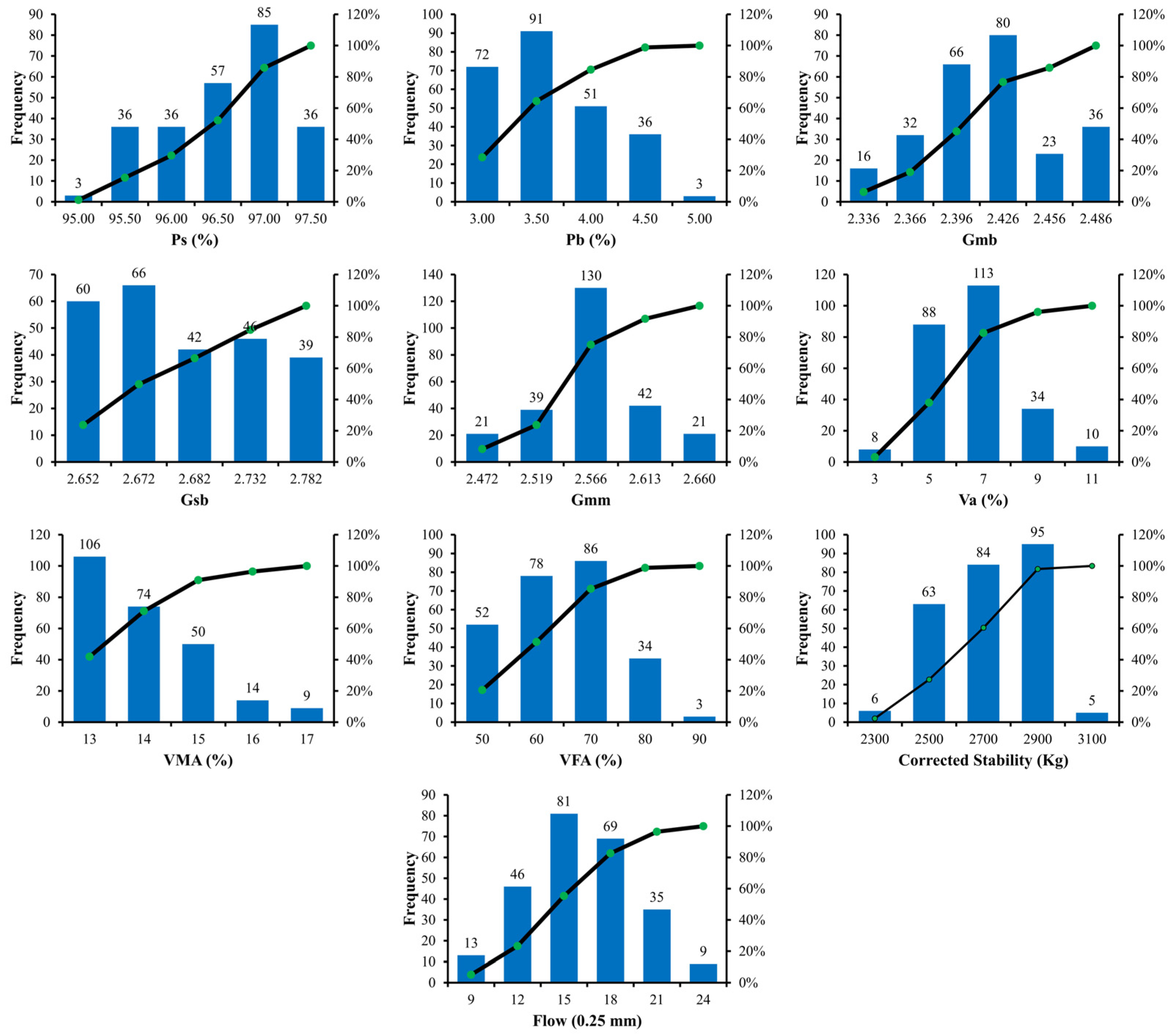
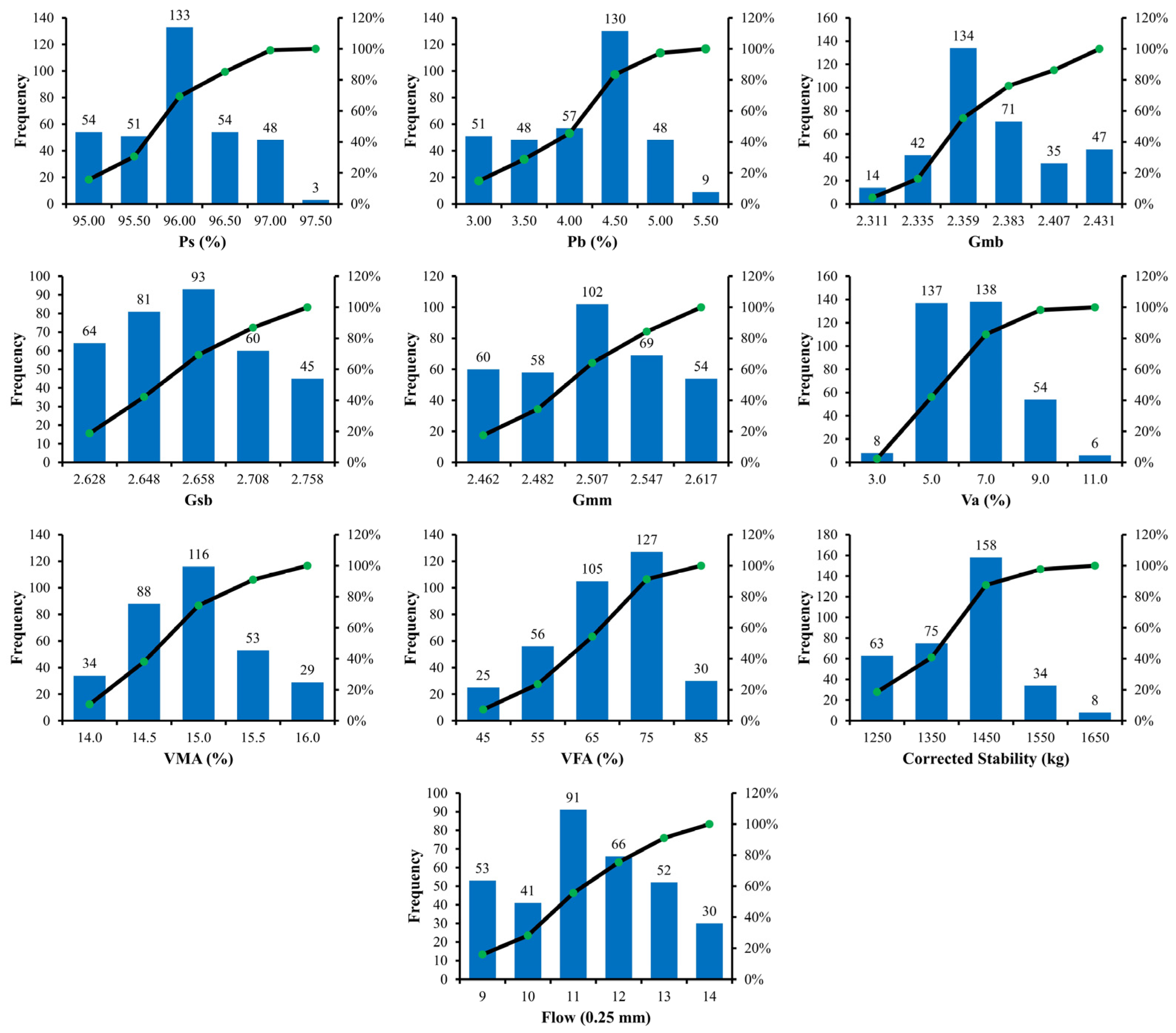
The selection of influential input parameters for the prediction of output parameters is the starting step in the development of a model. In order to develop the model, the parameters affecting MS and MF were selected. Numerous trials were made, and the results were calculated to assess the best and simplest influencing parameters for the development of the model. The equations below are used for the calculations of MS and MF of ABC and AWC of asphalt pavements.

MS = f(Ps (%), Pb (%), Gmb, Gsb, Gmm, Va (%), VMA (%), VFA (%))

MF = f(Ps (%), Pb (%), Gmb, Gsb, Gmm, Va (%), VMA (%), VFA (%))

Several fitting input parameters are required in MEP, which need to be identified before model development for a generalized and robust model. The fitting input parameters are carefully chosen, considering the previous recommendations and the trial-and-error approach [72]. The size of the population specifies the number of programs that are to be evolved. A model developed with large population size might be relatively accurate but it would be more complex and might take longer time to converge. Although, as size increases beyond a threshold limit, issues may arise regarding the overfitting of the model.

At the beginning, a subpopulation size of 10 and 100 generations were considered for the initiation of the project, with basic mathematical parameters, i.e., subtraction, addition, division, and multiplication. The parameters, including subpopulation and number of generations, were gradually increased in trials by addition of mathematical parameters in the models to reduce error size. The final selection of parameters for the four models, based on an acceptable error range, is shown in

Table 5. Parameters settings for MEP models.

Number of Subpopulations	50
Subpopulation Size	100
Code Length	50
Crossover Probability	0.9
Crossover Type	Uniform
Error Measure	MAE
Mathematical Operators	$+,-,\times , ÷, \mathrm{Power}, \mathrm{Sqrt}, \mathrm{Exp}, \mathrm{Sin}, \mathrm{Cos}, \mathrm{Tan}$
Mutation Probability	0.01
Tournament Size	2
Functions	0.5
Variables	0.5
Number of Generations	1000

.

The accuracy level that the model’s algorithm should achieve is determined by the number of generations prior to its termination. The larger the number of generations in a run, the less the statistical errors will be. Likewise, crossover and mutation rates indicate the offspring’s probability of undergoing these genetic operations. The range for the rate of crossover lies between 50–95%. Various combinations of the settings shown in Table 5 were tested on the data sample, and the optimum set of combinations was chosen based on the model’s overall performance attributes, which are shown in Table 5. Overfitting of the data is one of major challenges in AI-based modeling. The model’s efficiency is high, when using the original data, however, the efficiency reduces considerably when unseen data is used. To avoid this issue, it is recommended that the training model be tested on a testing or unseen dataset [73,74]. Consequently, the entire dataset was randomly divided into sets of training, validation and testing. In modeling, datasets of training and validation were processed. The validation model was then tested on the testing dataset, which was not included in the development of the model. The data distribution of all three datasets was assured to be consistent. For the current research study, 70%, 15%, and 15% of the data were used as training, testing, and validation, respectively. On all three datasets, the final developed models outperformed the competition. MEPX v 2021.08.05.0-beta, a commercially available computing tool, was used to implement the MEP algorithm.

The algorithm begins by creating a population of the most possible solutions. The process of the algorithm is iterative, and with each generation, it arrives closer to the solution. Within the solution population, each generation’s fitness is assessed. The algorithm of MEP continues to advance until the function for pre-specified fitness, such as root mean squared error (RMSE) or R, remains unchanged. For each trained model, the objective function (OF) was also assessed in this research study because it reflects the influence of R, RMSE and frequency of data points to quantify the overall efficiency. If the results of the model for all datasets, i.e., training, validation, and testing, are not accurate, the process is repeated, increasing the size and number of subpopulations incrementally. After that, the model is finalized based on the minimum value OF. It was determined that certain models performed better on the dataset of training than on the testing set, indicating overfitting of the proposed model, which ought to be avoided. The number of generations it takes for a model to evolve has an in impact on the mode’s accuracy. A model would keep evolving indefinitely in these types of algorithms due to induction of additional variables into the system. All the models in this research study were terminated at 1000 generations. Furthermore, an ideal model should meet the criteria for several performance indicators, as elaborated in the following discussion.

The effectiveness of the models was assessed by calculating several statistical error metrics. These statistical errors included for the assessment of the models were R, mean absolute error (MAE), RMSE, relative squared error (RSE), relative root mean square error (RRMSE), and the performance index (ρ). Moreover, another strategy to prevent the model’s overfitting was to choose an optimal model by reducing the value of OF, as advocated by Azim et al. [69], which is referred to as the fitness function. These statistical measures have the following Expressions (1)–(7):

$$\mathrm{R}=\frac{{{\displaystyle \sum }}_{\mathrm{i}=1}^{\mathrm{n}}\left({\mathrm{x}}_{\mathrm{i}}-{\overline{\mathrm{x}}}_{\mathrm{i}}\right)\left({\mathrm{p}}_{\mathrm{i}}-{\overline{\mathrm{p}}}_{\mathrm{i}}\right)}{\sqrt{{{\displaystyle \sum }}_{\mathrm{i}=1}^{\mathrm{n}}{\left({\mathrm{x}}_{\mathrm{i}}-{\overline{\mathrm{x}}}_{\mathrm{i}}\right)}^2{{\displaystyle \sum }}_{\mathrm{i}=1}^{\mathrm{n}}{\left({\mathrm{p}}_{\mathrm{i}}-{\overline{\mathrm{p}}}_{\mathrm{i}}\right)}^2}}$$

(1)

$$\mathrm{MAE}=\frac{{{\displaystyle \sum }}_{\mathrm{i}=1}^{\mathrm{n}}\left|{\mathrm{x}}_{\mathrm{i}}-{\mathrm{p}}_{\mathrm{i}}\right|}{\mathrm{n}}$$

(2)

$$\mathrm{RMSE}=\sqrt{\frac{{{\displaystyle \sum }}_{\mathrm{i}=1}^{\mathrm{n}}{\left({\mathrm{x}}_{\mathrm{i}}-{\mathrm{p}}_{\mathrm{i}}\right)}^2}{\mathrm{n}}}$$

(3)

$$\mathrm{RSE}=\frac{{{\displaystyle \sum }}_{\mathrm{i}=1}^{\mathrm{n}}{\left({\mathrm{p}}_{\mathrm{i}}-{\mathrm{x}}_{\mathrm{i}}\right)}^2}{{{\displaystyle \sum }}_{\mathrm{i}=1}^{\mathrm{n}}{\left({\overline{\mathrm{x}}}_{\mathrm{i}}-{\mathrm{x}}_{\mathrm{i}}\right)}^2}$$

(4)

$$\mathrm{RRMSE}=\frac{1}{\left|\overline{\mathrm{x}}\right|}\sqrt{\frac{{{\displaystyle \sum }}_{\mathrm{i}=1}^{\mathrm{n}}{\left({\mathrm{x}}_{\mathrm{i}}-{\mathrm{p}}_{\mathrm{i}}\right)}^2}{\mathrm{n}}}$$

(5)

$$\mathsf{\rho }=\frac{\mathrm{RRMSE}}{1+\mathrm{R}}$$

(6)

$$\mathrm{OF}=\left(\frac{{\mathrm{n}}_{\mathrm{T}}-{\mathrm{n}}_{\mathrm{TE}}}{\mathrm{n}}\right){\mathsf{\rho }}_{\mathrm{T}}+2\left(\frac{{\mathrm{n}}_{\mathrm{TE}}}{\mathrm{n}}\right){\mathsf{\rho }}_{\mathrm{TE}}$$

(7)

where p_i, x_i, ${\overline{\mathrm{p}}}_{\mathrm{i}}$ and ${\overline{\mathrm{x}}}_{\mathrm{i}}$, denote the ith predicted, experimental, mean predicted and mean experimental values, respectively, and the symbol n denotes the total number of values in the dataset used for the development of the models. The training and testing sets are denoted by abbreviations T and TE, respectively. An accurate model has a high R value, while the statistical errors are low. R has been recommended by the researchers to assess the linear dependency among input and output parameters [75], with a value greater than 0.8 indicating a decent correlation between experimental and predicted values [41,76]. Due to the insensitivity of R with the division and multiplication of outputs with a constant, it could not be considered solely as a measure for overall model efficiency. The average magnitude of errors can be measured using MAE and RMSE. Both parameters, however, have their own implication. In RMSE, errors are squared before average is estimated, giving larger errors more weight. A high RMSE value indicates that the amount of high-error predictions is significantly more than the expected and should be excluded. MAE, however, gives large errors a low weight and is always smaller than RMSE. Likewise, Despotovic et al., (2016) recommended that a model is considered to be outstanding if RRMSE values are between 0 and 0.10 and fair if the value is between 0.11 and 0.20 [77]. The range of values for OF and ρ is 0–infinity. If the values of ρ and OF are less than 0.2, the model can be considered as good [66]. While using OF, it considers three factors at the same time, i.e., R and RRMSE with relative percentage of data in various datasets (training and testing). As a result, a low value of OF indicates that the model’s overall performance is superior. As stated previously, numerous trial runs were carried out, and the models with the lowest values of OF stated in this research study. Additionally, the validation of developed models was also carried out using criteria suggested by various researchers, which are described in

Table 6. External validation criteria.

S. No.	Equation	Condition	Suggested by
1	$k=\frac{{{\displaystyle \sum }}_{\mathrm{i}=1}^{\mathrm{n}}\left({\mathrm{x}}_{\mathrm{i}}\times {\mathrm{p}}_{\mathrm{i}}\right)}{{{\displaystyle \sum }}_{\mathrm{i}}^{\mathrm{n}}{\mathrm{p}}_{\mathrm{i}}^2}$	0.85 < k < 1.15	Golbraikh and Tropsha, 2002
2	$k^{\prime }=\frac{{{\displaystyle \sum }}_{\mathrm{i}=1}^{\mathrm{n}}\left({\mathrm{x}}_{\mathrm{i}}\times {\mathrm{p}}_{\mathrm{i}}\right)}{{{\displaystyle \sum }}_{\mathrm{i}=1}^{\mathrm{n}}{\mathrm{x}}_{\mathrm{i}}^2}$	0.85 < k′ < 1.15	Golbraikh and Tropsha, 2002
3	$R_m={R^{\prime }}_0^2\times \left(1-\left|\sqrt{{R^{\prime }}_0^2-R_0^2}\right|\right)$	Rm > 0.5	Roy and Roy, 2008
	$R_0^2=1-\frac{{{\displaystyle \sum }}_{\mathrm{i}=1}^{\mathrm{n}}{\left({\mathrm{p}}_{\mathrm{i}}-{\mathrm{x}}_{\mathrm{i}}^{\mathrm{r}0}\right)}^2}{{{\displaystyle \sum }}_{\mathrm{i}=1}^{\mathrm{n}}{\left({\mathrm{p}}_{\mathrm{i}}-\overline{{\mathrm{p}}_{\mathrm{i}}}\right)}^2}$ ${R^{\prime }}_0^2=1-\frac{{{\displaystyle \sum }}_{\mathrm{i}=1}^{\mathrm{n}}{\left({\mathrm{x}}_{\mathrm{i}}-{\mathrm{p}}_{\mathrm{i}}^{\mathrm{r}0}\right)}^2}{{{\displaystyle \sum }}_{\mathrm{i}=1}^{\mathrm{n}}{\left({\mathrm{x}}_{\mathrm{i}}-\overline{{\mathrm{x}}_{\mathrm{i}}}\right)}^2}$ ${\mathrm{x}}_{\mathrm{i}}^{\mathrm{r}0}=\mathrm{k}\times {\mathrm{p}}_{\mathrm{i}}$ ${\mathrm{p}}_{\mathrm{i}}^{\mathrm{r}0}={\mathrm{k}}^{\prime }\times {\mathrm{e}}_{\mathrm{i}}$	$R_0^2 \cong 1$ ${R^{\prime }}_0^2 \cong 1$

.

4. Discussions

The models for MS and MF of ABC and AWC, respectively, were developed using MEP programming in MEPX v 2021.08.05.0-beta as already explained in Section 3. The results obtained from the equations obtained from the developed models and their analysis is described in this chapter.

Formulation of Mechanical Properties

The decoded mathematical equations for the calculation of corresponding properties based on eight input parameters are taken from MEP for ABC and AWC. The explicit expressions for MS and MF of ABC and MS and MF of AWC, respectively, are shown in Equations (8)–(11).

$$\mathrm{ABC}-\mathrm{MS}= \left(\mathrm{a}+\left(\left(\mathrm{a}+ \left(\left(\left(2\mathrm{d}\times \surd 2\mathrm{d}\right) + \mathrm{b}\right) - \left(\left(\left(2\mathrm{f}\right) + \left(\left(\sin \left(2\mathrm{d}\right) - \sin \left(\mathrm{d}\right)\right) \times 2\mathrm{d}\right)\right)- \tan \left(2\mathrm{f}\right)\right)\right)\right)-\left(\mathrm{e}\times \tan \left(\mathrm{d}^2\right)\right)\right)\right) + \mathrm{a}$$

(8)

where

$$\mathrm{a}=\tan \left({\mathrm{e}}^{{\mathrm{e}}^{\left(\sin \left(\mathrm{Ps} \left(\%\right)\right) -\sin \left(2\mathrm{Ps}\left(\%\right)\right)\right)}}\right)$$

$$\mathrm{b}=\tan \left(\tan \left(\tan \left(\mathrm{Ps}\left(\%\right) \times \mathrm{Ps}\left(\%\right)\right)\right)\right)$$

$$\mathrm{c}=\mathrm{Va} \left(\%\right) - \mathrm{VFA} \left(\%\right)$$

$$\mathrm{d}=\mathrm{Ps}\left(\%\right)$$

$$\mathrm{e}=\mathrm{Pb}\left(\%\right)$$

$$\mathrm{f}= \left(2\mathrm{d} + \sin \left(2\mathrm{d}\right)\right) + \left(\mathrm{c}\right)$$

$$\mathrm{ABC}-\mathrm{MF}= \left(\left(\left(\mathrm{e}^\left(\mathrm{a}/\mathrm{c}\right) + \cos \left(\mathrm{a}\right) + \mathrm{b}+\mathrm{d}\right)/\left(\mathrm{e} + \sin \left(\mathrm{b}\right)\right) - \sin \left(\cos \left(\mathrm{a}\right)\times \mathrm{a}\right)\right) -\left(\mathrm{f}/\left(\cos \left(\mathrm{a}\right) \times \mathrm{a} + \mathrm{a}\right)\right)/\left(\cos \left(\mathrm{a}\right) \times \mathrm{a}\right)\right)- \sin \left(\mathrm{b}\right)$$

(9)

where

$$\mathrm{a}={\mathrm{Gsb}}^{\mathrm{Gsb}}+{ \mathrm{Gsb}}^{\mathrm{Gsb}}$$

$$\mathrm{b}={\mathrm{e}}^{\cos \left(\mathrm{a}\right)}{}^{\mathrm{Gmm}}$$

$$\mathrm{c}=\frac{\mathrm{VFA} \left(\%\right)}{\mathrm{Gmm}}$$

$$\mathrm{d}=\mathrm{VFA} \left(\%\right) \times \mathrm{Pb} \left(\%\right)$$

$$\mathrm{e}=\sqrt{\mathrm{VFA} \left(\%\right) \times \mathrm{Pb} \left(\%\right)}$$

$$\mathrm{f}=\mathrm{VFA} \left(\%\right) + \mathrm{Gmm}$$

$$\mathrm{AWC}-\mathrm{MS} = \left(\cos \left(\mathrm{c}\right) \times \mathrm{h}\right)+\left(\left(\left(2\mathrm{i} - \mathrm{a}\right) + \left(\left(\cos \left(\mathrm{f}\right)\times \mathrm{g}\right) + \left(\left(\mathrm{c} \times \mathrm{d}\right) + \tan \left(\mathrm{c}\right)\right)\right)\right) + \cos \left(\mathrm{f}\right) \times \mathrm{h}\right)$$

(10)

where

$$\mathrm{a}= \mathrm{Ps} \left(\%\right) + \cos \left(\mathrm{VMA} \left(\%\right)\right)$$

$$\mathrm{b}=\cos \left(\mathrm{VMA} \left(\%\right)\right) + \cos \left(\mathrm{VMA} \left(\%\right)\right)$$

$$\mathrm{c}={\mathrm{e}}^{\mathrm{Gsb}}$$

$$\mathrm{d}=\mathrm{Ps} \left(\%\right) + \sin \left(\mathrm{a} - \mathrm{b}\right)$$

$$\mathrm{e}=\mathrm{Pb} \left(\%\right)$$

$$\mathrm{f}=\mathrm{VMA} \left(\%\right)$$

$$\mathrm{g}=\mathrm{Ps} \left(\%\right)$$

$$\mathrm{h}=\mathrm{e} \times \left(\mathrm{a} - \left(\mathrm{d} - \mathrm{f}\right)\right)$$

$$\mathrm{i}= \left(\sin \left(\mathrm{g}\right)\times \mathrm{d}\right) + \sqrt{\mathrm{b}}$$

$$\mathrm{AWC}-\mathrm{MF}= \left(\left(\mathrm{b} - \left(\sin \left(\mathrm{a}\right) - \mathrm{c}\right)\right)- \mathrm{d}\right) + \frac{\sin \left(\sin \left(\mathrm{c}\right)\right)}{{\left(\tan \left(\sin \left(\mathrm{a}\right)\right) + \mathrm{e}\right)}^{\left(\mathrm{b} + \sin \left(\mathrm{a}\right)\right) - \mathrm{f}}}$$

(11)

where

$$\mathrm{a}={\mathrm{e}}^{\mathrm{Gsb}}$$

$$\mathrm{b}={\mathrm{Gmb}}_{}$$

$$\mathrm{c}=\mathrm{VMA} \left(\%\right)$$

$$\mathrm{d}=\mathrm{Va} \left(\%\right)$$

$$\mathrm{e}=\mathrm{Gmm}$$

$$\mathrm{f}={\mathrm{e}}^{\sin \left({\mathrm{e}}^{{\mathrm{e}}^{\mathrm{Gsb}}}\right)}$$

For Equations (8)–(11):

ABC–MS = Marshall Stability of Asphalt Base Course;

ABC–MF = Marshall Flow of Asphalt Base Course;

AWC–M = Marshall Stability of Asphalt Wearing Course;

AWC–MF = Marshall Flow of Asphalt Wearing Course;

Ps (%) = Aggregates;

Pb (%) = Asphalt Content;

Gmb = Bulk Specific Gravity of Compacted Aggregate;

Gsb = Bulk Specific Gravity of Aggregate;

Gmm = Maximum Specific Gravity Paving Mix;

Va (%) = Air Voids;

VMA (%) = Voids in Mineral Aggregate;

VFA (%) = Voids Filled by Bitumen.

The comparison between experimental and predicted values of MS and MF of ABC and MS and MF of AWC are shown in Figure 3 and Figure 4 below for all of the datasets, i.e., training, validation and testing. Additionally, regression line expression is also displayed in these graphs. For an ideal scenario, the slope of the regression line should be close to 1. It can be considered from Figure 3 and Figure 4 below that the developed models have a significant correlation between the values of predicted and experimental data as manifested by the slopes of 0.9742, 0.9759, and 0.9624 for training, validation, and testing, respectively, for MS of ABC; 0.9742, 0.9759, and 0.9624 for training, validation, and testing, respectively, for MF of ABC; 0.9530, 0.9714, and 0.9029 for training, validation, and testing, respectively, for MS of AWC; and 0.9581, 0.9783, and 0.9727 for training, validation, and testing, respectively, for MF of AWC. The developed models have been trained thoroughly on the input parameters in order to effectively predict the values of MS and MF for ABC and AWC, respectively. Furthermore, for the data points for all three datasets, the results are quite comparable to one another and close to an ideal fit, showing that the models have been well trained and possess strong generalization capability, i.e., the performance of the models on unseen data will be equally well. The models have performed exceptionally well on the testing data. This demonstrates that the problem regarding the overfitting of the data points employed for modeling has been greatly removed in all the models. Moreover, the number of data points employed for such empirical models has a significant impact on the applicability and accuracy of such models [78]. The largest number of points, i.e., 241, have been chosen in the collated database for MS and MF of AWC; hence, minimum errors with high accuracy have been achieved.

5. Results

5.1. Performance Evaluation of MEP Models

The volume of datasets used in developing the models are also important because the reliability of developed models is dependent on these. The literature recommends a ratio of greater than 5 for the number of data points to the number of input parameters used in both unseen and training (testing and validation) stages [66,79,80]. For the training stage, the ABC and AWC models have a ratio of 22.13 and 30.13, respectively. While in the testing stage, the ABC and AWC models have values of 5.75 and 6.38, respectively. Statistical measures such as R, MAE, RSE, RMSE, RRMSE, OF, and ρ are used to evaluate the performance of the developed models, as explained in Section 3.

Table 7. Statistical measures for training, testing, and validation.

Model	Dataset	R	MAE	RMSE	RSE	RRMSE	ρ	OF
ABC–MS	Training	0.96	36.30	46.62	0.07	0.01	0.004	0.033
	Validation	0.96	33.51	41.39	0.08	0.03	0.017
	Testing	0.97	36.94	46.71	0.06	0.03	0.017
ABC–MF	Training	0.97	0.62	0.80	0.05	0.01	0.004
	Validation	0.98	0.53	0.73	0.05	0.04	0.018
	Testing	0.96	0.71	0.90	0.09	0.03	0.017
AWC–MS	Training	0.95	26.65	33.72	0.13	0.01	0.003	0.046
	Validation	0.97	24.64	30.55	0.07	0.02	0.012
	Testing	0.90	29.59	43.32	0.29	0.03	0.015
AWC–MF	Training	0.96	0.37	0.47	0.09	0.01	0.003
	Validation	0.98	0.34	0.40	0.05	0.02	0.012
	Testing	0.97	0.31	0.41	0.06	0.03	0.013

below shows the results of these statistical measures for training, testing, and validation for the ABC and AWC models.

It is seen from Table 7 that experimental and predicted values have a strong correlation, as evident by an R of 0.96, 0.97, 0.95, and 0.96 for training; 0.96, 0.98, 0.97, and 0.98 for validation; and 0.97, 0.96, 0.90, and 0.97 for testing datasets of ABC–MS (MS of ABC), ABC–MF (MF of ABC), AWC–MS (MS of AWC), and AWC–MF (MF of AWC) models, respectively.

The results of MAE, RMSE, and RSE for all three of the datasets are considerably low and close, which indicates the model’s strong generalization capacity and high accuracy. The MAE is 36.30, 33.5, and 36.94 for ABC–MS; 0.62, 0.53, and 0.71 for ABC–MF; 26.65, 24.64, and 29.59 for AWC–MS; and 0.37, 0.34, and 0.31 for AWC–MF for all three datasets, respectively. The values of RMSE for ABC–MS are 46.62, 41.39 and 46.71; for ABC–MF are 0.80, 0.73, and 0.90; for AWC–MS are 33.72, 30.55, and 43.22; and for AWC–MF are 0.47, 0.40, and 0.41, respectively for all three datasets. The results of the data revealed that the values of MAE are lower than RMSE, indicating that the criteria of analysis described in Section 3 is satisfied. The models developed for estimation of ABC–MS, ABC–MF, AWC–MS and AWC–MF can be labeled as excellent based on RRMSE estimates, as values are less 0.10, i.e., 0.01, 0.03, and 0.03 for ABC–MS; 0.01, 0.04, and 0.03 for ABC–MF; 0.01, 0.02, and 0.03 for AWC–MS; and 0.01, 0.02, 0.03, respectively, for the three datasets of all models.

The results of ρ is less than 0.20 for all three datasets for all four developed models, demonstrating that all four developed models are reliable and have the capability to predict output parameters.

For the ABC and AWC models, the values of OF are 0.033 and 0.046, respectively. These values are almost near to zero, verifying overall performance and demonstrating that the problems regarding the overfitting for the proposed models has been addressed properly.

To analyze the statistics of absolute errors, the datasets for all four developed models are plotted in Figure 5, Figure 6, Figure 7 and Figure 8 below, together with absolute errors in their respective points of the datasets. The mean error of predicted values for ABC–MF and AWC–MF is 0.62 and 0.35, with a maximum error of 3.59 and 1.64, respectively. Out of 253 data points for ABC–MS, only four points have a value greater than 100 kg, which accounts for 1.58% of the total data points, while for AWC–MS, only eight points have a value greater than 80 kg out of 343 data points, which accounts for 2.33% of the total data points. According to the findings, it was concluded that for ABC–MS, ABC–MF, AWC–MS, and AWC–MF, 85% of the results have errors less than 67 kg, 1.05 (0.25 mm) and 48 kg, 0.63 (0.25 mm), respectively.

5.2. External Validation

Table 8. Results of external validation.

Model	k	k′	Rm	R20	R’20
ABC–MS	1.0008	0.9989	0.9887	0.9999	0.9997
ABC–MF	0.9996	0.9975	0.9894	1.0000	0.9999
AWC–MS	0.9994	1.0000	0.9913	0.9999	1.0000
AWC–MF	0.9985	1.00	1.0000	1.0000	1.0000

below shows the results of the additional criteria utilizing external validation of the developed models. The slopes of the regression lines (k or k′) running from the origin have been suggested to be close to one [81]. A confirmed indicator (Rm) was proposed by Roy and Roy (2008) as a measure of the model’s external predictability. When Rm > 0.5, this criteria is satisfied [82]. Table 8 below indicates the all four models have satisfied the criteria considered in the external validation of the models, indicating that the all the developed models are credible, and these are not a mere correlation between input and output parameters.

5.3. Parametric Analysis

In the case of model development based on AI, numerous analyses are required to guarantee that models are strong and that their performance is well across a variety of datasets. A higher performance of the current datasets, i.e., training, testing, and validation, does not imply that the models are superior overall. Numerous research has advocated for the use of parametric analysis, and it is used in this research study to determine whether the models are well trained and not only a correlation of the input and output parameters. All the input parameters are set to their mean value, and the output variation is plotted against the change in one of the input parameters over its entire range. This procedure is carried out for each of the input parameters separately. The results of the parametric analysis for MS of ABC and AWC and MF of ABC and AWC for their respective developed models are shown in Figure 9 and Figure 10, respectively.

The equations of MS and MF of ABC and AWC as developed by MEP does not use all the input parameters in each equation. The MEP algorithms have chosen the input parameters that have given the best results. Based on the developed equations of MEP models, only the parameters drawn in Figure 9 and Figure 10 are used in the equations developed by MEP and have a significant impact on the output parameters.

5.3.1. Marshall Stability Analysis

Figure 9 shows that as Ps (%), Pb (%), and Va (%) increases, MS increases to a point and subsequently drops. Additionally, it has been witnessed in the collected datasets that when Ps (%), Pb (%), and Va (%) increase, MS first increases and then drops. MS is likewise seen to decrease linearly when Gsb and VMA (%) increase. The collected dataset also shows that as Gsb and VMA (%) increases, MS decreases. MS increases linearly as VFA (%) increases. In addition, it has been observed in the collected datasets that when VFA (%) increases, MS increases as well. Previous research studies have found similar trends in the parametric analysis of MS [8].

5.3.2. Marshall Flow Analysis

MF increases with increasing Pb (%), Gmb, and VFA (%), as shown in Figure 10. In the collected datasets, it was also discovered that when Pb (%), Gmb, and VFA (%) increases, MF increase as well. MF decreases linearly when Gsb, Gmm, Va (%), and VMA (%) increase. The collected datasets also show that as Gsb, Gmm, Va (%), and VMA (%) increase, MF decreases. Previous research studies have found similar trends in the parametric analysis of MS [8].

6. Conclusions

This research study utilizes MEP, an innovative AI technique in the area of pavement engineering to develop predictive models for MS and MF of M2DM for the ABC and AWC of flexible pavements. For this reason, wide and comprehensive datasets were produced from various projects in Pakistan. The researchers developed high-precision models, and the following are the main conclusions of this research study:

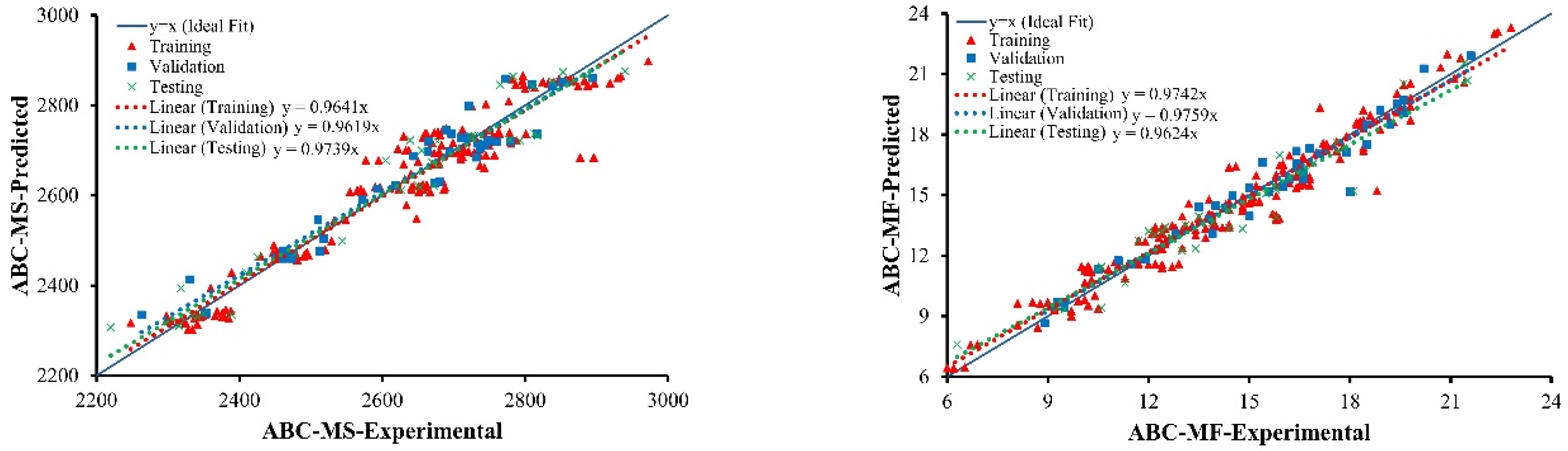
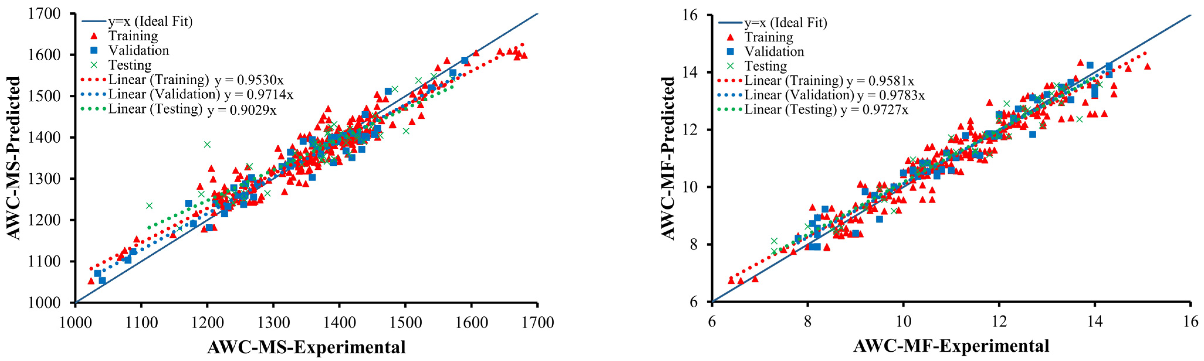
• The developed models have produced results that are consistent with the experimental data and function equally well for unknown data.
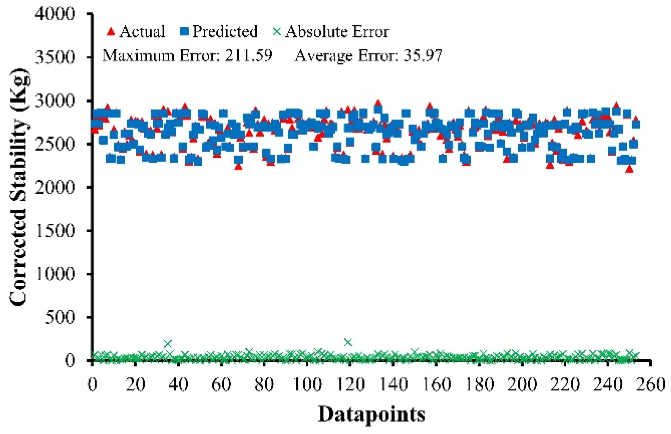
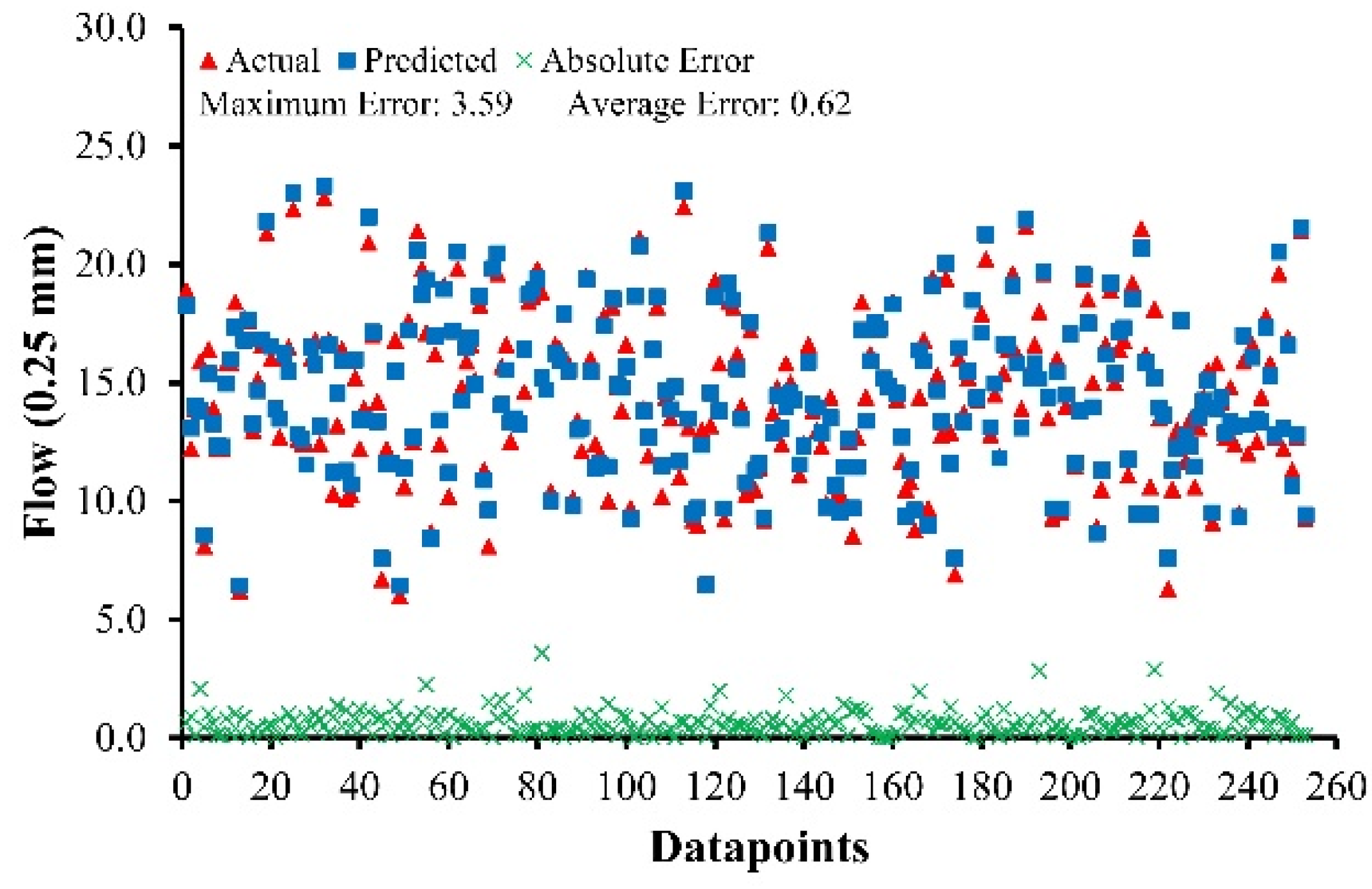
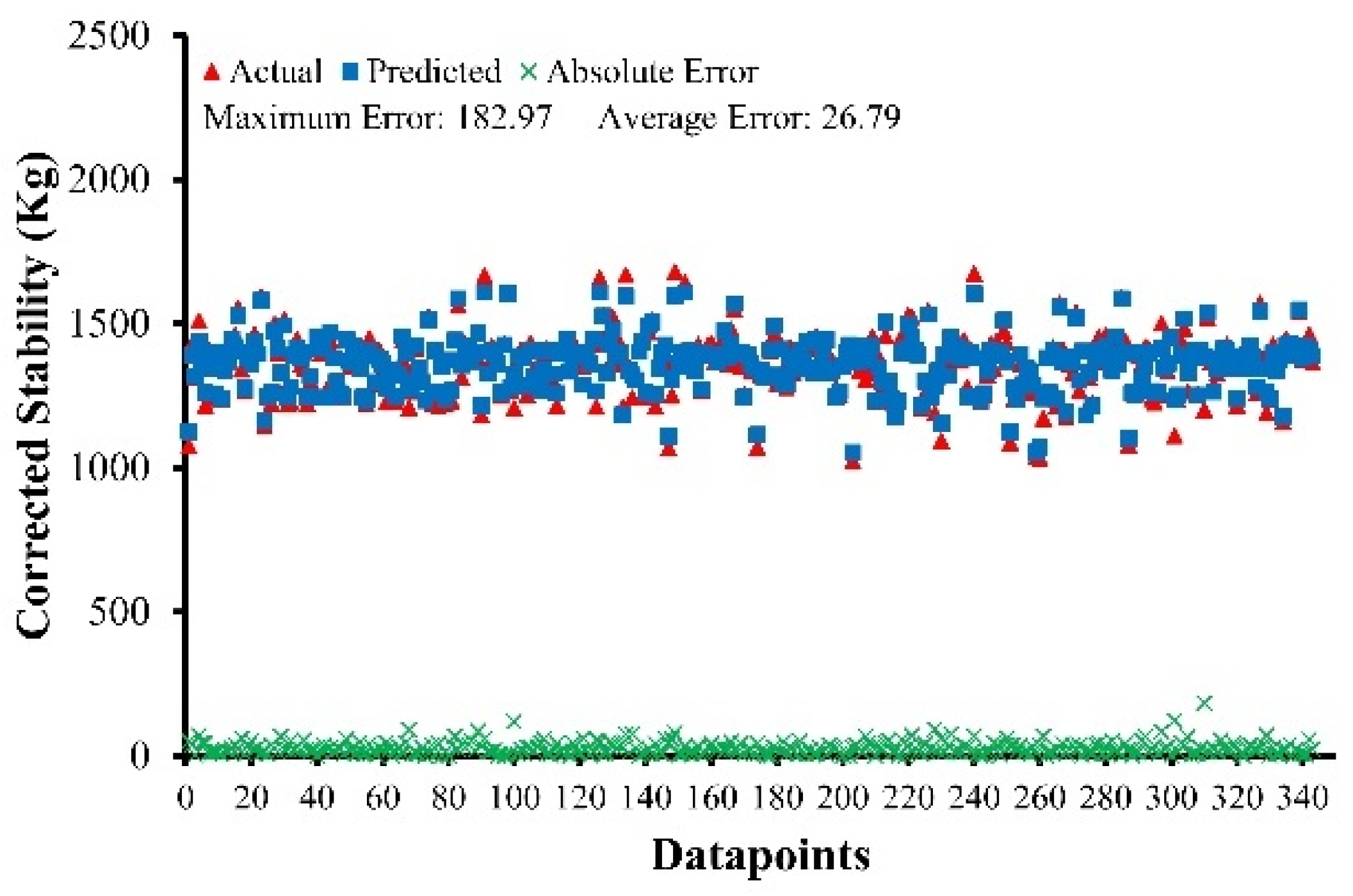
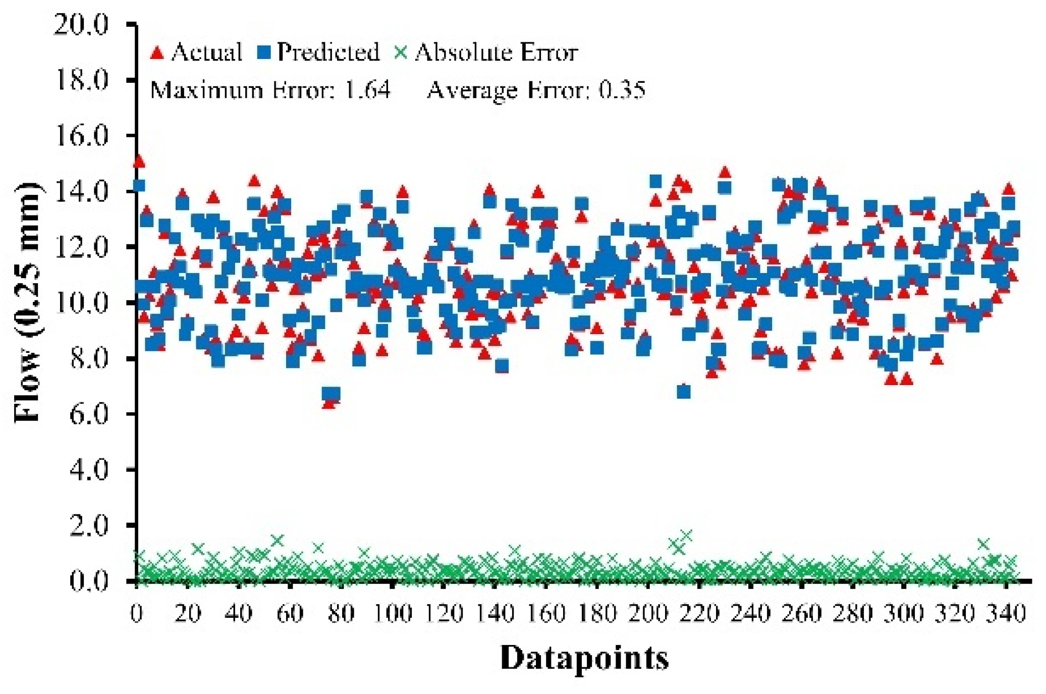
• Various performance measures such as R, RRMSE, RSE, RMSE, MAE were used to assess the reliability and correction of the developed models. Furthermore, OF and ρ showed highly generalization capability of the developed models, with the issue of overfitting effectively addressed. The results of the statistical parameters validated the accuracy of the proposed MEP developed models.
• The value of R lies in between 0.90 and 0.98 for MS and MF of ABC and AWC. MAE ranges from 24.64 to 36.94 kg for MS of ABC and AWC, while it ranges from 0.31 (0.25 mm) to 0.71 (0.25 mm) for MF of ABC and AWC.
• The developed models also met a number of external validation criteria taken from the literature.
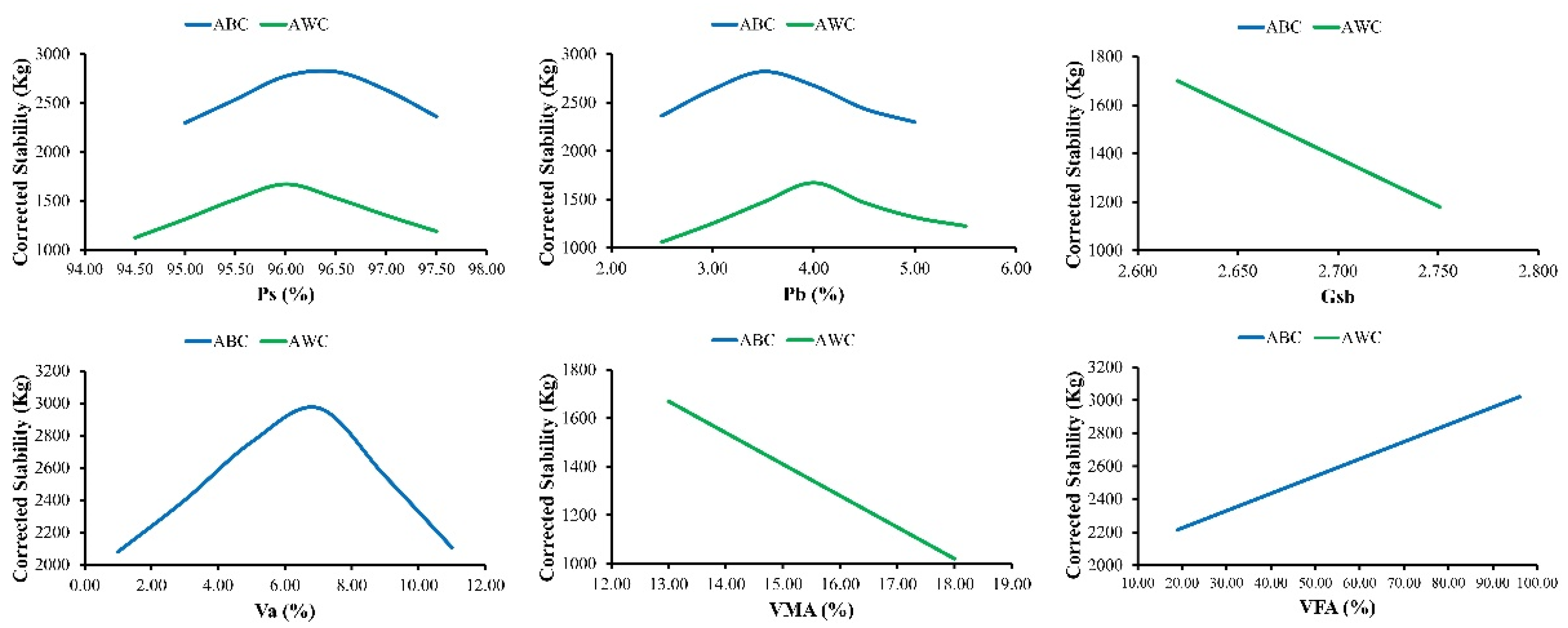
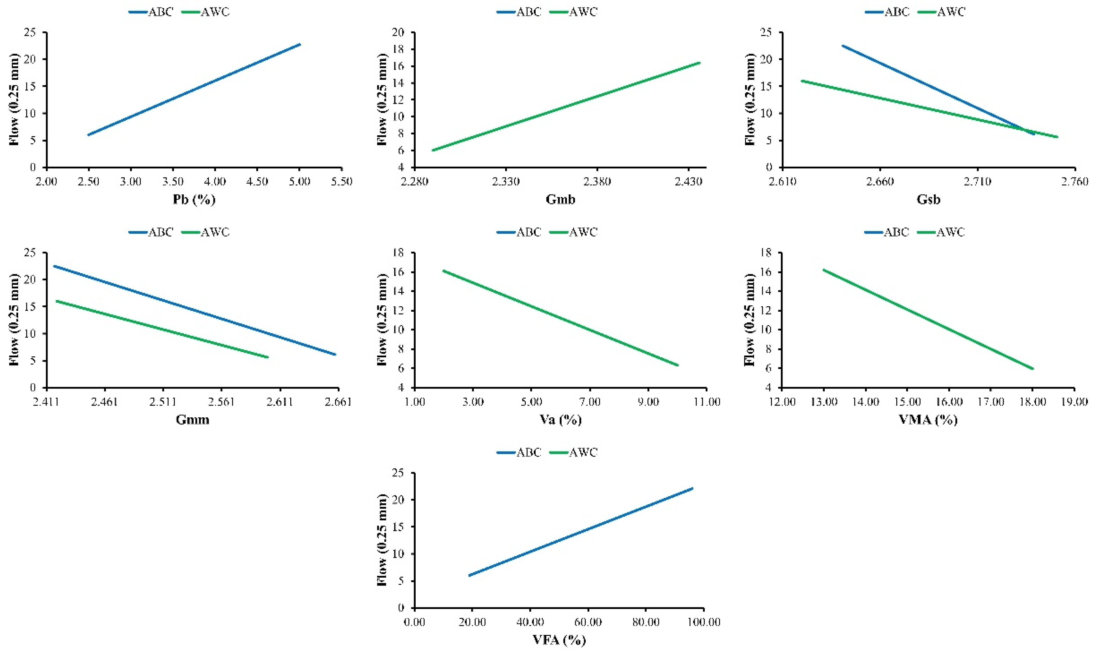
• The models developed have successfully incorporated input parameters and have the capability to predict the trends of MS and MF for flexible pavements, as revealed from the parametric study.
• It is convincing from the modeling approach being proposed, i.e., MEP in conjunction with validation parameters, that MEP can be utilized for predicting the Marshall parameters.

It is suggested that different AI techniques such as SVM, Ensemble random forest regression, eXtreme gradient boosting (XGBoost), GEP, and ANFIS should be used to predict MS and MF and should then be compared to each other to see which AI technique is more efficient in predicting MS and MF.

It is recommended that bitumen with different penetration grades such as 85/100 and 45/50 be tested on AI-based Marshall parameter modeling.

The most influential parameter in M2DM is the grading of aggregates, whereas the impact of grading on M2DM has to be discussed by various researchers. Hence, finding the influence of different types of grading on Marshall parameters using various AI methods is also recommended.

References

1. Asphalt Institute. MS-2 Asphalt Mix Design Methods; Asphalt Institute: Lexington, KY, USA, 2014. [Google Scholar]
2. Zumrawi, M.M.; Edrees, S.A.S. Comparison of Marshall and Superpave asphalt design methods for Sudan pavement mixes. Int. J. Sci. Tech. Adv. 2016, 2, 29–35. [Google Scholar]
3. Ministry of Communications. National Highway Authority, Government of Pakistan; Ministry of Communications: Islamabad, Pakistan, 2009; pp. 301-1–301-3d.
4. Kuloǧlu, N. Effect of astragalus on characteristics of asphalt concrete. J. Mater. Civ. Eng. 1999, 11, 283–286. [Google Scholar] [CrossRef]
5. Hınıslıoğlu, S.; Ağar, E. Use of waste high density polyethylene as bitumen modifier in asphalt concrete mix. Mater. Lett. 2004, 58, 267–271. [Google Scholar] [CrossRef]
6. Azarhoosh, A.; Pouresmaeil, S. Prediction of Marshall Mix Design Parameters in Flexible Pavements Using Genetic Programming. Arab. J. Sci. Eng. 2020, 45, 8427–8441. [Google Scholar] [CrossRef]
7. Alsugair, A.M.; Al-Qudrah, A.A. Artificial neural network approach for pavement maintenance. J. Comput. Civ. Eng. 1998, 12, 249–255. [Google Scholar] [CrossRef]
8. Tapkın, S.; Çevik, A.; Uşar, Ü. Prediction of Marshall test results for polypropylene modified dense bituminous mixtures using neural networks. Expert Syst. Appl. 2010, 37, 4660–4670. [Google Scholar] [CrossRef]
9. Milad, A.A. Development of a Hybrid Machine Learning Model for Asphalt Pavement Temperature Prediction. IEEE Access 2021, 9, 158041–158056. [Google Scholar] [CrossRef]
10. Aslam, F. Compressive strength prediction of rice husk ash using multiphysics genetic expression programming. Ain Shams Eng. J. 2021, 13, 101593. [Google Scholar] [CrossRef]
11. Zhao, T.H.; Khan, M.I.; Chu, Y.M. Artificial neural networking (ANN) analysis for heat and entropy generation in flow of non-Newtonian fluid between two rotating disks. Math. Methods Appl. Sci. 2021. [Google Scholar] [CrossRef]
12. Zha, T.-H. A fuzzy-based strategy to suppress the novel coronavirus (2019-NCOV) massive outbreak. Appl. Comput. Math. 2021, 20, 160–176. [Google Scholar]
13. Chu, H.-H.; Zhao, T.-H.; Chu, Y.-M. Sharp bounds for the Toader mean of order 3 in terms of arithmetic, quadratic and contraharmonic means. Math. Slovaca 2020, 70, 1097–1112. [Google Scholar] [CrossRef]
14. Zhao, T.-H.; He, Z.-Y.; Chu, Y.-M. On some refinements for inequalities involving zero-balanced hypergeometric function. AIMS Math 2020, 5, 6479–6495. [Google Scholar] [CrossRef]
15. Zhao, T.-H.; Wang, M.-K.; Chu, Y.-M. A sharp double inequality involving generalized complete elliptic integral of the first kind. AIMS Math 2020, 5, 4512–4528. [Google Scholar] [CrossRef]
16. Zhao, T.-H. Quadratic transformation inequalities for Gaussian hypergeometric function. J. Inequalities Appl. 2018, 2018, 251. [Google Scholar] [CrossRef] [PubMed] [Green Version]
17. Zhao, T.-H. On approximating the quasi-arithmetic mean. J. Inequalities Appl. 2019, 2019, 42. [Google Scholar] [CrossRef]
18. Ozgan, E. Artificial neural network based modelling of the Marshall Stability of asphalt concrete. Expert Syst. Appl. 2011, 38, 6025–6030. [Google Scholar] [CrossRef]
19. Baldo, N.; Manthos, E.; Miani, M. Stiffness modulus and marshall parameters of hot mix asphalts: Laboratory data modeling by artificial neural networks characterized by cross-validation. Appl. Sci. 2019, 9, 3502. [Google Scholar] [CrossRef] [Green Version]
20. Shah, S.A.R. Marshall stability and flow analysis of asphalt concrete under progressive temperature conditions: An application of advance decision-making approach. Constr. Build. Mater. 2020, 262, 120756. [Google Scholar] [CrossRef]
21. Saffarzadeh, M.; Heidaripanah, A. Effect of asphalt content on the marshall stability of asphalt concrete using artificial neural networks. Sci. Iran. 2009, 16, 98–105. [Google Scholar]
22. Morova, N. Modeling Marshall Stability of light asphalt concretes fabricated using expanded clay aggregate with Artificial Neural Networks. In Proceedings of the 2012 International Symposium on Innovations in Intelligent Systems and Applications, Trabzon, Turkey, 2–4 July 2012. [Google Scholar]
23. Morova, N. Modelling Marshall Stability of fiber reinforced asphalt mixtures with ANFIS. In Proceedings of the 2017 IEEE International Conference on Innovations in Intelligent Systems and Applications (INISTA), Gdynia, Poland, 3–5 July 2017. [Google Scholar]
24. SERİN, S. The Fuzzy Logic Model for the Prediction of Marshall Stability of Lightweight Asphalt Concretes Fabricated using Expanded Clay Aggregate. Süleyman Demirel Üniversitesi Fen Bilimleri Enstitüsü Derg. 2013, 17, 163–172. [Google Scholar]
25. Ozgan, E. Fuzzy logic and statistical-based modelling of the Marshall Stability of asphalt concrete under varying temperatures and exposure times. Adv. Eng. Softw. 2009, 40, 527–534. [Google Scholar] [CrossRef]
26. Tsompanakis, Y. Stability Prediction of Asphaltic Concrete Mixes Using Multiple Additive Regression Trees. In Proceedings of the Fourth International Conference on Soft Computing Technology in Civil, Structural and Environmental Engineering; Civil-Comp Press: Prague, Czech Republic, 2015. [Google Scholar]
27. Nguyen, H.-L. Development of hybrid artificial intelligence approaches and a support vector machine algorithm for predicting the marshall parameters of stone matrix asphalt. Appl. Sci. 2019, 9, 3172. [Google Scholar] [CrossRef] [Green Version]
28. Khuntia, S. Prediction of Marshall parameters of modified bituminous mixtures using artificial intelligence techniques. Int. J. Transp. Sci. Technol. 2014, 3, 211–227. [Google Scholar] [CrossRef] [Green Version]
29. Ghanizadeh, A.R. Predicting flow number of asphalt mixtures based on the marshall mix design parameters using multivariate adaptive regression spline (MARS). Int. J. Transp. Eng. 2020, 7, 433–448. [Google Scholar]
30. Yan, K.-Z.; Ge, D.-D.; Zhang, Z. Support vector machine models for prediction of flow number of asphalt mixtures. Int. J. Pavement Res. Technol. 2014, 7, 31. [Google Scholar]
31. Sharifi, S.; Abrishami, S.; Gandomi, A.H. Consolidation assessment using multi expression programming. Appl. Soft Comput. 2020, 86, 105842. [Google Scholar] [CrossRef]
32. Alavi, A.H. Multi expression programming: A new approach to formulation of soil classification. Eng. Comput. 2010, 26, 111–118. [Google Scholar] [CrossRef]
33. Chu, H.-H. Sustainable use of fly-ash: Use of gene-expression programming (GEP) and multi-expression programming (MEP) for forecasting the compressive strength geopolymer concrete. Ain Shams Eng. J. 2021, 12, 3603–3617. [Google Scholar] [CrossRef]
34. Gandomi, A.H. New design equations for elastic modulus of concrete using multi expression programming. J. Civ. Eng. Manag. 2015, 21, 761–774. [Google Scholar] [CrossRef] [Green Version]
35. Iqbal, M.F. Sustainable utilization of foundry waste: Forecasting mechanical properties of foundry sand based concrete using multi-expression programming. Sci. Total Environ. 2021, 780, 146524. [Google Scholar] [CrossRef]
36. Zhang, Q. Predicting cement compressive strength using double-layer multi-expression Programming. In Proceedings of the 2012 Fourth International Conference on Computational and Information Sciences, Chongqing, China, 17–19 August 2012. [Google Scholar]
37. Abdalla, A.; Salih, A. Implementation of multi-expression programming (MEP), artificial neural network (ANN), and M5P-tree to forecast the compression strength cement-based mortar modified by calcium hydroxide at different mix proportions and curing ages. Innov. Infrastruct. Solut. 2022, 7, 153. [Google Scholar] [CrossRef]
38. Heshmati, A. A multi expression programming application to high performance concrete. World Appl. Sci. J. 2008, 5, 215–223. [Google Scholar]
39. Amin, M.N. Multigene Expression Programming Based Forecasting the Hardened Properties of Sustainable Bagasse Ash Concrete. Materials 2021, 14, 5659. [Google Scholar] [CrossRef] [PubMed]
40. Wang, H.-L.; Yin, Z.-Y. High performance prediction of soil compaction parameters using multi expression programming. Eng. Geol. 2020, 276, 105758. [Google Scholar] [CrossRef]
41. Gandomi, A.H.; Alavi, A.H.; Yun, G.J. Formulation of uplift capacity of suction caissons using multi expression programming. KSCE J. Civ. Eng. 2011, 15, 363–373. [Google Scholar] [CrossRef]
42. Koza, J.R. Genetic Programming: On the Programming of Computers by Means of Natural Selection; MIT Press: Cambridge, MA, USA, 1992; Volume 1. [Google Scholar]
43. Banzhaf, W. Genetic Programming: An Introduction: On the Automatic Evolution of Computer Programs and Its Applications; Morgan Kaufmann Publishers Inc.: Burlington, MA, USA, 1998. [Google Scholar]
44. Back, T. Evolutionary Algorithms in Theory and Practice: Evolution Strategies, Evolutionary Programming, Genetic Algorithms; Oxford University Press: Oxford, UK, 1996. [Google Scholar]
45. Oltean, M.; Dumitrescu, D. Multi expression programming. J. Genet. Program. Evolvable Mach. Kluwer Second. Tour Rev. 2002. [Google Scholar] [CrossRef]
46. Oltean, M.; Grosan, C. A comparison of several linear genetic programming techniques. Complex Syst. 2003, 14, 285–314. [Google Scholar]
47. Khan, M.A. Simulation of Depth of Wear of Eco-Friendly Concrete Using Machine Learning Based Computational Approaches. Materials 2022, 15, 58. [Google Scholar] [CrossRef]
48. Ceylan, H. Backcalculation of full-depth asphalt pavement layer moduli considering nonlinear stress-dependent subgrade behavior. Int. J. Pavement Eng. 2005, 6, 171–182. [Google Scholar] [CrossRef]
49. Ceylan, H. Accuracy of predictive models for dynamic modulus of hot-mix asphalt. J. Mater. Civ. Eng. 2009, 21, 286–293. [Google Scholar] [CrossRef] [Green Version]
50. Vapnik, V. The Nature of Statistical Learning Theory; Springer Science & Business Media: Berlin/Heidelberg, Germany, 2013. [Google Scholar]
51. Alavi, A.H. Formulation of flow number of asphalt mixes using a hybrid computational method. Constr. Build. Mater. 2011, 25, 1338–1355. [Google Scholar] [CrossRef]
52. Alawi, M.; Rajab, M. Determination of optimum bitumen content and Marshall stability using neural networks for asphaltic concrete mixtures. In Proceedings of the 9th WSEAS International Conference on Computers, World Scientific and Engineering Academy and Society (WSEAS), Athens, Greece, 11–13 July 2005. [Google Scholar]
53. Serin, S. Determining amount of bituminous effects on asphalt concrete strength with artificial intelligence and statistical analysis methods. In Proceedings of the 2011 International Symposium on Innovations in Intelligent Systems and Applications, Istanbul, Turkey, 15–18 June 2011. [Google Scholar]
54. Bagheri, M. Investigating plant uptake of organic contaminants through transpiration stream concentration factor and neural network models. Sci. Total Environ. 2021, 751, 141418. [Google Scholar] [CrossRef] [PubMed]
55. Abdolrasol, M.G. Artificial Neural Networks Based Optimization Techniques: A Review. Electronics 2021, 10, 2689. [Google Scholar] [CrossRef]
56. Nazeer, M. Theoretical study of MHD electro-osmotically flow of third-grade fluid in micro channel. Appl. Math. Comput. 2022, 420, 126868. [Google Scholar] [CrossRef]
57. Oltean, M.; Groşan, C. Evolving evolutionary algorithms using multi expression programming. In Proceedings of the European Conference on Artificial Life, Dortmund, Germany, 14–17 September 2003. [Google Scholar]
58. Khan, M.A. Geopolymer Concrete Compressive Strength via Artificial Neural Network, Adaptive Neuro Fuzzy Interface System, and Gene Expression Programming with K-Fold Cross Validation. Front. Mater. 2021, 8, 621163. [Google Scholar] [CrossRef]
59. Khan, S. Predicting the Ultimate Axial Capacity of Uniaxially Loaded CFST Columns Using Multiphysics Artificial Intelligence. Materials 2022, 15, 39. [Google Scholar] [CrossRef]
60. Faris, H.; Mirjalili, S.; Aljarah, I. Automatic selection of hidden neurons and weights in neural networks using grey wolf optimizer based on a hybrid encoding scheme. Int. J. Mach. Learn. Cybern. 2019, 10, 2901–2920. [Google Scholar] [CrossRef]
61. Ferreira, C. Gene Expression Programming: Mathematical Modeling by an Artificial Intelligence; Springer: Berlin/Heidelberg, Germany, 2006; Volume 21. [Google Scholar]
62. Azim, I. Semi-analytical model for compressive arch action capacity of RC frame structures. In Structures; Elsevier: Amsterdam, The Netherlands, 2020. [Google Scholar]
63. Azim, I. Prediction of catenary action capacity of RC beam-column substructures under a missing column scenario using evolutionary algorithm. KSCE J. Civ. Eng. 2021, 25, 891–905. [Google Scholar] [CrossRef]
64. Chu, Y.-M. Combined impact of Cattaneo-Christov double diffusion and radiative heat flux on bio-convective flow of Maxwell liquid configured by a stretched nano-material surface. Appl. Math. Comput. 2022, 419, 126883. [Google Scholar] [CrossRef]
65. Khan, M.A. Compressive strength of fly-ash-based geopolymer concrete by gene expression programming and random forest. Adv. Civ. Eng. 2021, 2021, 6618407. [Google Scholar] [CrossRef]
66. Gandomi, A.H.; Roke, D.A. Assessment of artificial neural network and genetic programming as predictive tools. Adv. Eng. Softw. 2015, 88, 63–72. [Google Scholar] [CrossRef]
67. Maeda, T. How to rationally compare the performances of different machine learning models? PeerJ Prepr. 2018. [Google Scholar] [CrossRef]
68. Abunama, T. Leachate generation rate modeling using artificial intelligence algorithms aided by input optimization method for an MSW landfill. Environ. Sci. Pollut. Res. 2019, 26, 3368–3381. [Google Scholar] [CrossRef] [PubMed]
69. Azim, I. Prediction Model for Compressive Arch Action Capacity of RC Frame Structures under Column Removal Scenario Using Gene Expression Programming. In Structures; Elsevier: Amsterdam, The Netherlands, 2020. [Google Scholar]
70. Li, P. Sustainable Use of Chemically modified Tyre Rubber in Concrete: Machine Learning based Novel Predictive Model. Chem. Phys. Lett. 2022, 793, 139478. [Google Scholar] [CrossRef]
71. Smith, G.N. Probability and statistics in civil engineering. In Collins Professional and Technical Books; Collins: London, UK, 1986; Volume 244. [Google Scholar]
72. Mousavi, S. A data mining approach to compressive strength of CFRP-confined concrete cylinders. Struct. Eng. Mech. 2010, 36, 759. [Google Scholar] [CrossRef]
73. Pyo, J. Estimation of heavy metals using deep neural network with visible and infrared spectroscopy of soil. Sci. Total Environ. 2020, 741, 140162. [Google Scholar] [CrossRef]
74. Qiu, R. Water temperature forecasting based on modified artificial neural network methods: Two cases of the Yangtze River. Sci. Total Environ. 2020, 737, 139729. [Google Scholar] [CrossRef]
75. Nguyen, T. Deep neural network with high-order neuron for the prediction of foamed concrete strength. Comput. Aided Civ. Infrastruct. Eng. 2019, 34, 316–332. [Google Scholar] [CrossRef]
76. Gandomi, A.H. Nonlinear genetic-based models for prediction of flow number of asphalt mixtures. J. Mater. Civ. Eng. 2011, 23, 248–263. [Google Scholar] [CrossRef]
77. Despotovic, M. Evaluation of empirical models for predicting monthly mean horizontal diffuse solar radiation. Renew. Sustain. Energy Rev. 2016, 56, 246–260. [Google Scholar] [CrossRef]
78. Gholampour, A.; Gandomi, A.H.; Ozbakkaloglu, T. New formulations for mechanical properties of recycled aggregate concrete using gene expression programming. Constr. Build. Mater. 2017, 130, 122–145. [Google Scholar] [CrossRef]
79. Ali Khan, M. Application of Gene Expression Programming (GEP) for the Prediction of Compressive Strength of Geopolymer Concrete. Materials 2021, 14, 1106. [Google Scholar] [CrossRef] [PubMed]
80. Khan, M.A. Application of random forest for modelling of surface water salinity. Ain Shams Eng. J. 2021, 13, 101635. [Google Scholar] [CrossRef]
81. Golbraikh, A.; Tropsha, A. Beware of q2! J. Mol. Graph. Model. 2002, 20, 269–276. [Google Scholar] [CrossRef]
82. Roy, P.P.; Roy, K. On some aspects of variable selection for partial least squares regression models. QSAR Comb. Sci. 2008, 27, 302–313. [Google Scholar] [CrossRef]
Figure 1. Distribution of input parameters for ABC.
Buildings 12 00314 g001
Figure 2. Distribution of input parameters for AWC.
Buildings 12 00314 g002
Figure 3. Comparison between experimental and predicted values of ABC.
Buildings 12 00314 g003
Figure 4. Comparison between experimental and predicted values of AWC.
Buildings 12 00314 g004
Figure 5. Absolute errors of ABC–MS.
Buildings 12 00314 g005
Figure 6. Absolute errors of ABC–MF.
Buildings 12 00314 g006
Figure 7. Absolute errors of AWC–MS.
Buildings 12 00314 g007
Figure 8. Absolute errors of AWC–MF.
Buildings 12 00314 g008
Figure 9. Parametric analysis of MS–ABC–AWC.
Buildings 12 00314 g009
Figure 10. Parametric analysis of MF–ABC–AWC.
Buildings 12 00314 g010