Abstract
In this work, analytical pushover curves for concentric braced steel frames with active tension diagonal bracings (X-CBF) are proposed. A pushover “spindle”, characterized by two trilinear analytical capacity curves defined for an X-CBF system subjected to prefixed lateral forces distribution, is defined. The curves are able to grasp the elasto-plastic behavior of the X-CBFs. The reliability of this analytical proposal is verified by a series of numerical comparisons obtained through an accurate finite element model, calibrated on the basis of experimental results. The proposal is extended to whole single- and multi-storey structures, showing a good correspondence with the numerical results of the analyzed case studies.
1. Introduction
It is known that the use of X-CBF systems with active tension diagonal bracings is widespread in the seismic areas because of their great efficiency against horizontal actions. In particular, during an earthquake, the energy is dissipated through the diagonals that have high plasticization in tension and buckling phenomena in compression, while beams and columns remain in general elastics [1,2,3].
This type of bracing is particularly used in steel buildings, both for single-floor systems (industrial buildings) and multi-storey residential and office buildings, due to its high dissipative capacity and cheapness of realization.
As is well known, the hysteretic behavior of the X-CBF is strongly influenced by buckling in compression, plasticization in tension and pinching phenomenon when there is the inversion of the seismic actions. Current codes treat differently the buckling phenomena of the brace in compression. The EN1998-1 (also referred to as Eurocode 8 or EC8, [1]), in a seismic elastic analysis, requires to consider the contributions of the in-tension diagonals only. This design methodology of X-CBF steel structures may lead to uneconomical and poorly efficient structures, as underlined in several past studies [4,5,6]. If the designer wants to consider also the compressed members, it is necessary to perform non-linear static or dynamic analyses, more accurate and complete but surely more complex than the elastic ones [7]. The American AISC 341-16 [2] requires to consider also the compressed diagonal. Two separate analyses are requested: one elastic, in which all braces are assumed to resist the seismic action with their expected strength in tension or compression (pre-buckling phase), and a second one, plastic, in which the in-tension diagonal is with its expected strength and the compressed one with its expected post-buckling strength [2,8]. The Canadian [9] and Japanese [10] codes, in a similar way, require two different checks for the two behavior phases, with different relationships. In [11], a simplified design method based on a linear elastic response spectrum analysis is presented, by considering both the braces and using a modified stiffness of the system, as obtained by an appropriate reduction of the braces area.
The hysteretic behavior of the CBF has been deeply analyzed in the last thirty years, both theoretically and experimentally. Many studies, as in [12,13,14,15], have demonstrated that an X-CBF subjected to monotonic or cyclic horizontal increasing actions is characterized by a three-phase behavior (Figure 1). In the first phase (“Pre-Buckling phase”), the braces are both active; in the second one (“Post-Buckling phase”), the compressed braces are buckled; in the third one (“Plastic phase”), the braces in tension plasticize.
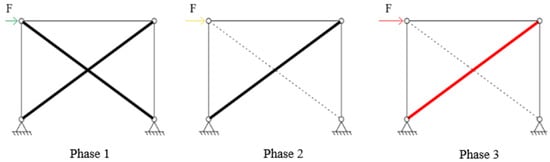
Figure 1.
Schematization of the three phases of a X-CBF response under an increasing load; phase 1: elastic behavior with both diagonals active; phase 2: elastic behavior with a single active diagonal; phase 3: plastic phase.
The modelization of the non-linear behavior for the different phases is complex and may lead to errors of assessment [12,16]. In particular, three different categories of modeling have been developed [7,17]: phenomenological models; beam–column elements with different approaches to describing the interaction between axial forces and second-order effects; and three-dimensional finite element models. The first ones are the simplest, but they need a calibration on experimental data. In contrast, the last ones are not generally used in structural engineering applications because of their complexity in terms of computational effort. Thus, commonly, the second ones are the most used and allow obtaining accurate results without an excessive computational load. In these cases, the X-CBF is modeled through frame elements connected by hinges. The plasticity can be concentrated or distributed along the element, according to a fiber modeling.
If we want to perform a pushover analysis on an X-CBF, it is required to adequately consider the three different behavior phases. In this work, a method to get a trilinear pushover “spindle” is proposed and described in Section 2. Then, an X-CBF model is validated through a real experimental test [12] by considering a beam-elements model with distributed plasticity, according to a fiber modeling (Section 3). The accuracy of the proposal is demonstrated on different X-CBFs by varying the slenderness of the brace (Section 4). Finally, the proposal is extended to mono- and multi-storey steel buildings (Section 5), by analyzing different case studies (Section 6).
2. Trilinear Proposed Curves
As seen in the introduction, a one-floor X-CBF has a three-phase behavior (Figure 1):
- In phase 1, the X-CBF has a high lateral stiffness ( ), everything remains elastic, and there are no buckling phenomena;
- In phase 2, the structure loses about half of its lateral stiffness because of the buckling of the compressed diagonal; by neglecting the contribution of this one, the lateral stiffness becomes ;
- In phase 3, the system loses all its stiffness () because of the yielding of the diagonal in tension.
For the presence of these different phases, the cyclic behavior is characterized by important phenomena of pinching in and out of the plane of the X-CBF. The second-phase stiffness of an X-CBF, under the hypothesis of neglecting the post-critical contribution of the compressed diagonal, can be easily calculated on the basis of the configuration reported in Figure 2. This solution is obtained, by omitting intermediate steps, as:
with:
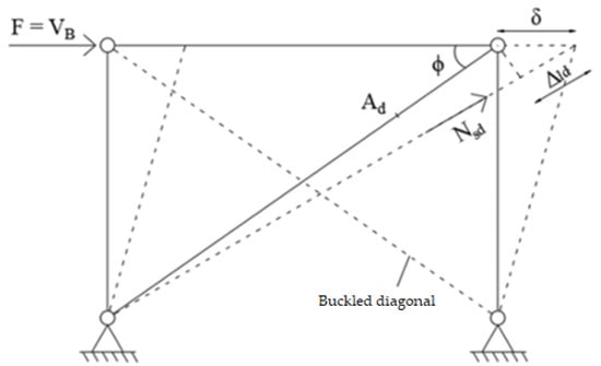
Figure 2.
Calculation scheme for the second-phase stiffness .
- : shear base force;
- : top displacement;
- : Young’s modulus;
- : diagonal cross-section;
- : beam–column angle;
- : diagonal length.
The stiffness of the first-phase can be considered as two times the one of the second-phase :
Furthermore, it is possible to calculate the critical load for the entire system with two diagonals (that divide the first from the second phase):
where is the critical load for a single compressed diagonal, calculable as defined in [1]:
with:
- : reduction coefficient for stability problems;
- : normalized slenderness of the diagonal;
- : imperfection coefficient;
- : reduction coefficient for local buckling.
The shear value that brings the diagonal in tension at the yielding is:
By considering the compressed diagonal contributor, three different post-critical behaviors are, in general, identifiable (Figure 3):
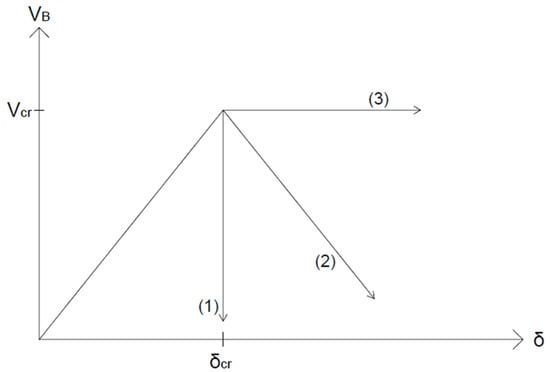
Figure 3.
Possible post-critical behavior of the compressed diagonal.
- (1)
- Instantaneous loss of load;
- (2)
- Relevant softening after the elastic phase;
- (3)
- Plastic behavior caused by relevant post-critical resources of the compressed diagonal.
It can be observed that:
- A squat diagonal () will show a behavior similar to that of curve (3);
- A slender diagonal () will show a behavior like curve (1), typical of cables, for example;
- A medium-slender diagonal () will show an intermediate behavior, like curve (2).
The behavior of the whole CBF is the sum of both compressed and in-tension diagonals. The global behavior can be seen in Figure 4, where new parameters are defined:
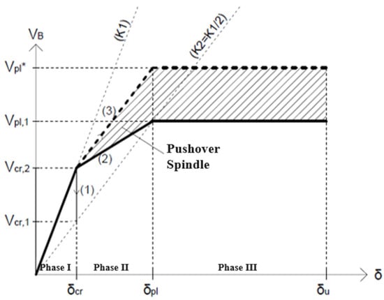
Figure 4.
Pushover global graph, sum of the curves of the single members.
: critical shear for the single-diagonal system
: plastic shear obtained by considering the plastic contributor of the in-tension diagonal with the critical contributor of the compressed one
: story drift corresponding to the yielding state in a single-diagonal CBF model
The initial part of the capacity curve (phase I) is characterized by slope until the critical load . The behavior in phase II depends on the post-critical trend of the compressed diagonal. Three types of behavior can be identified:
- If the load discharge is instantaneous (line (1) in Figure 4), a vertical line is followed, until the intersection with the line with stiffness in correspondence to the shear value ;
- If the compressed diagonal has a pseudo-plastic behavior, line (3) is followed, with a slope equal to =/2, reaching the third phase in correspondence to shear value and displacement;
- If the compressed diagonal has medium slenderness (), it is possible to reach the third phase with curve (2) characterized by a plastic shear lower than .
Trend (1), which is an extreme case typical of cables, is neglected, including for the restrictions imposed by the current regulations. Therefore, it is expected that the response of an X-CBF will be included between the two analytical limit curves (see Figure 4):
- The “Lower-bound” curve, characterized by a second phase with a stiffness less than half of , and achievable by connecting the point in correspondence to with the one with
- The “Upper-bound” curve, characterized by a higher second-phase stiffness, equal to , and with a plastic shear value equal to .
The field between the two curves represents a “spindle” in which the solutions are possible. The “lower-bound” curve can be then selected as a capacity curve by operating in a safe way.
Limit values such as those given in the FEMA274 [18] can be taken as the ultimate displacement of phase III (Table 1).

Table 1.
FEMA274 drift limits.
3. Numerical Validation
As previously said, the correct modeling of a single-storey X-CBF is generally complex because of the many variables involved. For this purpose, the X-CBF of Wakabayashi’s experimental test [12] was analyzed. The test consists of a cyclic imposed displacement (Figure 5) on an unloaded X-CBF, identified as BC0. The single-storey X-CBF (represented in Figure 6; the geometric and mechanic characteristics are given in Table 2) is composed of an H 175 × 175 × 7.5 × 11 column fixed at the base and connected with an H 250 × 125 × 6 × 9 beam. Beam–column nodes are rigid and with complete resistance because they are welded and stiffened with diagonal plates. Diagonals are H 100 × 50 × 4 × 6 profiles, connected in the middle; one is continuous, and the other is broken into two parts. The connections on the corners are not explained in Wakabayashi’s report; thus, the geometries given in [19] were considered (Figure 7).
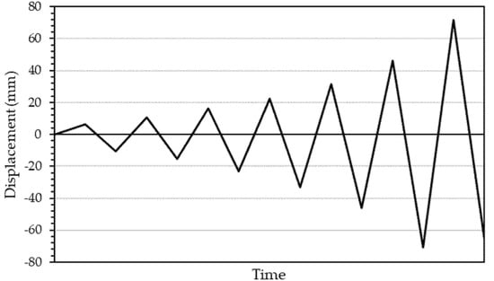
Figure 5.
Experimental loading protocol of Wakabayashi’s test.
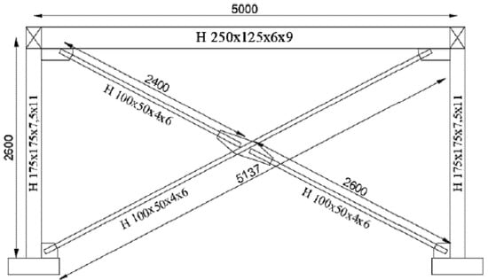
Figure 6.
Representation of the X-CBF used in Wakabayashi’s test (measurements in mm). Some like “x” means “×”.
Table 2.
Geometric and mechanic features of the steel profiles used in the test.
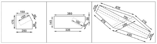
Figure 7.
Details of connection plates (in order: base, top and diagonal intersection; measurements in mm).
The modeling was performed with the SAP2000 code [20] using fiber frame elements with diffuse plasticity. The initial modeling of the X-CBF follows what is reported in [19]: a frame fixed to the base, with rigid column–beam nodes, hinged diagonals at the ends and initial geometric imperfections equal to L/1000, applied in the plane of the CBF, in the middle of each diagonal semi-length L (Figure 8). The imperfection value was taken from the Dicleli and Calik relationship [21].
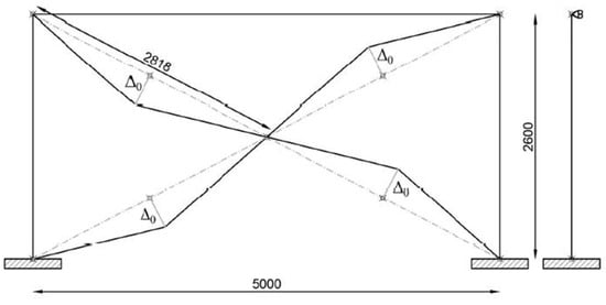
Figure 8.
Representation of the initial imperfections (measurements in mm).
The semi-diagonals were divided into eight equal elements and beams and columns into four (Figure 9). Fiber plastic hinges were then assigned to each element by considering their entire length.
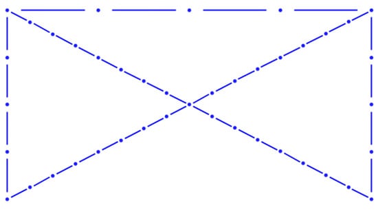
Figure 9.
Representation of the discretization of the elements.
With this modeling, the experimental cycles showed a pinching slightly higher than the experimental results. For this reason, a second model was adopted, with rigid parts in correspondence to the nodal zones (Figure 10).
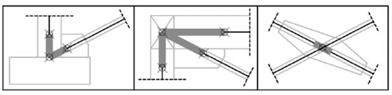
Figure 10.
Definition of the rigid parts on the nodal zones.
As can be seen in Figure 11, the cyclic numerical response (red continuous line) results very close to the experimental one (black continuous line); thus, the model is considered validated.
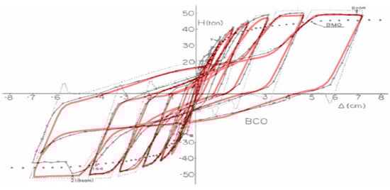
Figure 11.
Comparison between the results of the numerical model implemented with SAP2000 (red continuous line) and the experimental test (BC0 curve—black continuous line; background image taken from [12]).
4. Numerical Comparisons
Once the model was validated, several pushover analyses were carried out using different profiles for the diagonals (Table 3). A model with all pinned joints was considered.
Table 3.
Different profiles and normalized slenderness of the diagonals.
The pushover analysis results are given below (Figure 12, Figure 13, Figure 14, Figure 15 and Figure 16), compared with the proposed analytical curves. It can be clearly observed that the higher the normalized slenderness of the diagonal is, the tighter the analytical spindle is. However, the numerical curves are always inside the proposed pushover spindle. The analytical curves are therefore generally able to accurately describe the real three-phase behavior of the single X-CBF.
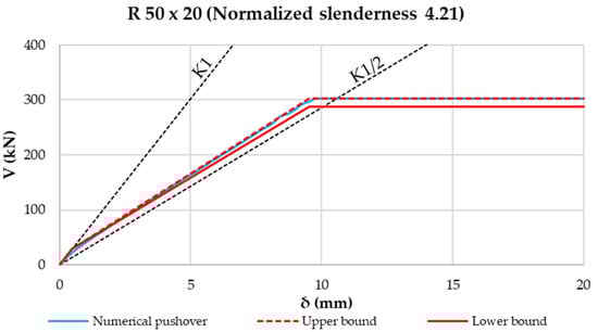
Figure 12.
Comparison between analytical pushover curves and numerical one for the profile R 50 × 20. Some like “x” means “×”.
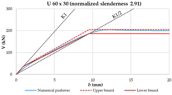
Figure 13.
Comparison between analytical pushover curves and numerical one for the profile U 60 × 30. Some like “x” means “×”.
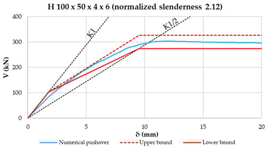
Figure 14.
Comparison between analytical pushover curves and numerical one for the profile H 100 × 50 × 4 × 6. Some like “x” means “×”.
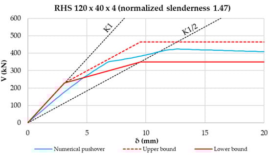
Figure 15.
Comparison between analytical pushover curves and numerical one for the profile RHS 120 × 40 × 4. Some like “x” means “×”.
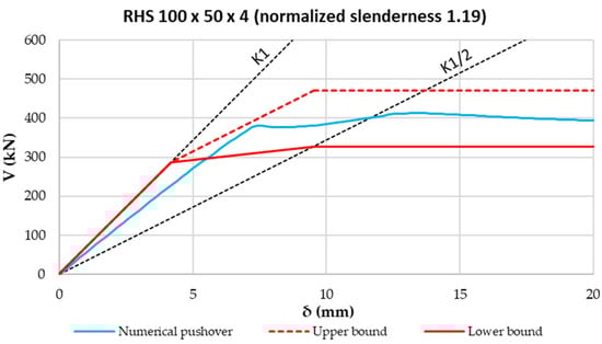
Figure 16.
Comparison between analytical pushover curves and numerical one for the profile RHS 100 × 50 × 4. Some like “x” means “×”.
5. Application to Mono- and Multi-Storey Buildings
Consequent to what was just carried out, it was possible to obtain an estimation of the overall behavior of an entire structure.
For the mono-floor building case, assuming equal and symmetrical X-CBFs, critical and plastic shear of the whole structure are calculated by multiplying the quantities of the single X-CBFs by the number of X-CBFs in the analyzed direction.
The corresponding critical and plastic displacements are the same as the single X-CBF:
The resulting upper-bound curve is obtained by substituting in the previous relationships, for each X-CBF, the shear value with .
For the multi-storey building, an optimal design condition, for which buckling and plasticization occur simultaneously at each level of the building, is assumed. Thus, critical and plastic shear of the whole-building lower-bound curve is considered equal to the corresponding values of the first level only (L1; values calculated as in the mono-storey building case):
Like in the one-floor building case, the upper-bound curve is obtained by substituting the plastic shear with .
For a multi-storey building, stiffnesses are determined by adding in series the individual stiffnesses of all levels. Then and displacements are obtained with Equations (17) and (18).
The summary of the proposed approach is presented in Table 4.
Table 4.
Summary table of the relationships defining the proposed analytical curves.
6. Case Studies
Four case studies with different X-CBF dispositions were analyzed, considering:
- Mono- or multi-storey buildings;
- Behavior factor equal to 1 or 4.
The structures were considered to be located in Tolmezzo (Udine, Italy), on a class B ground, with topographic class T1 and a 5% damping coefficient (according to the NTC2018 classification, [22]). The nominal design life was considered equal to 50 years, and the category of use was II. The collapse limit state (SLC) was adopted as an ultimate limit state. The normalized slenderness of diagonals was guaranteed between 1.3 and 2, as indicated in §7.5.5 of the NTC2018 [22]. In addition, for multi-storey buildings, the ratio between maximum and minimum over-strength must be less or equal to 25%.
6.1. One-Floor Case Studies
The geometrical characteristics (Figure 17, Figure 18 and Figure 19), the loads (Table 5) and the profiles used (Table 6) for the analyzed case studies are given below.
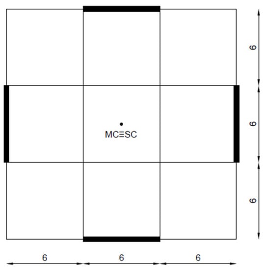
Figure 17.
Plan of the one-floor building (measurements in m).
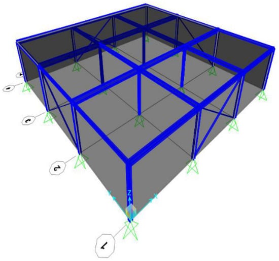
Figure 18.
Mono-story building model with SAP2000.
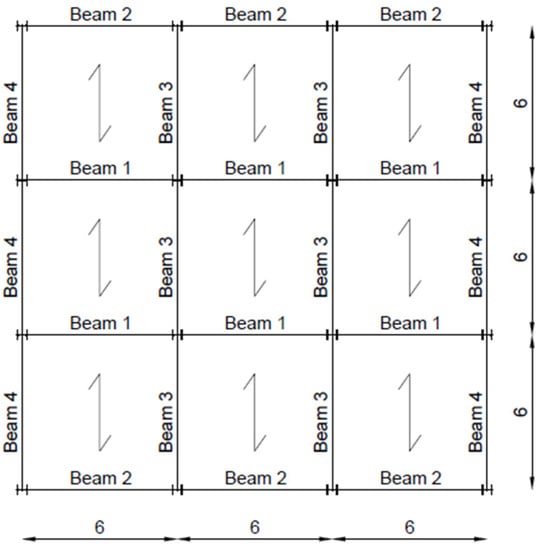
Figure 19.
Warping of the floors and numbering of the beams (valid for all case studies; measurements in m).
Table 5.
Loads applied to the one-floor case studies.
Table 6.
Beam and column cross-sections of the one-floor case studies after vertical static analysis design.
The results, given in Figure 20 and Figure 21, show a good correspondence between the numerical curve and the analytical spindle in terms of both stiffness and strength. The numerical curve is in both cases inside the spindle, with initial stiffness similar to the analytical one and the value of the plastic strength intermediate to the limit curves.
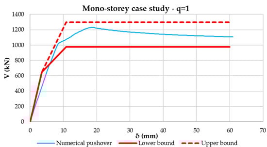
Figure 20.
Comparison between numerical pushover curve and analytical spindle for the mono-storey building case study with structure factor equal to 1.
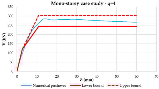
Figure 21.
Comparison between numerical pushover curve and analytical spindle for the mono-storey building case study with structure factor equal to 4.
6.2. Multi-Story Case Studies
The geometrical characteristics (Figure 22 and Figure 23), the loads (Table 7) and the profiles used (Table 8, Table 9 and Table 10) for the multi-storey case studies are given below. The characteristics of floors and the numbering of the beams are the same as the mono-storey cases (Figure 19). The structural design was made considering spectral plateau acceleration.
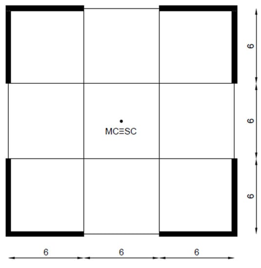
Figure 22.
Plan of the multi-storey building (measurements in m).
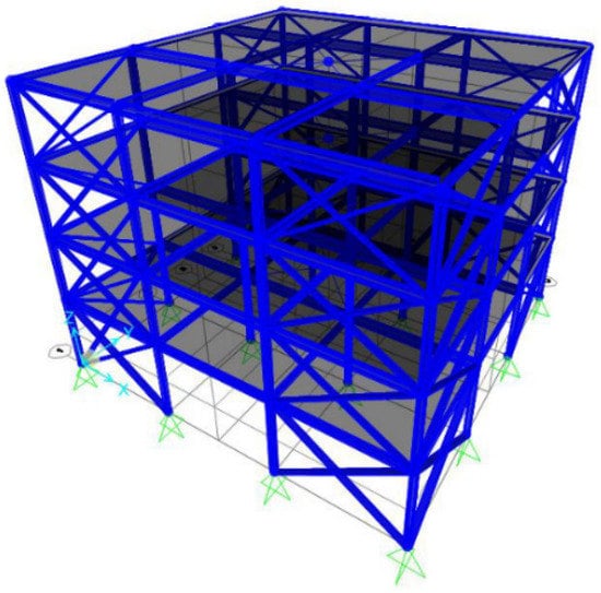
Figure 23.
Multi-storey building model with SAP2000.
Table 7.
Loads applied to the multi-storey case studies.
Table 8.
Beam and column cross-sections of the multi-storey case studies after vertical static analysis design.
Table 9.
Diagonal cross-sections of the multi-storey case study with structure factor equal to 1.
Table 10.
Diagonal cross-sections of the multi-storey case study with structure factor equal to 4.
The numerical curves fall well within the analytical pushover spindle also for the multi-story cases, as can be seen in Figure 24 and Figure 25. The stiffness values and strength limits correctly caught the real behavior of the structures. The lower-bound curve can be then assumed as the capacity curve for the design of the structure.
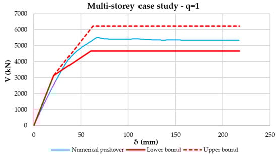
Figure 24.
Comparison between numerical pushover curve and analytical spindle for the multi-storey building case study with structure factor equal to 1.
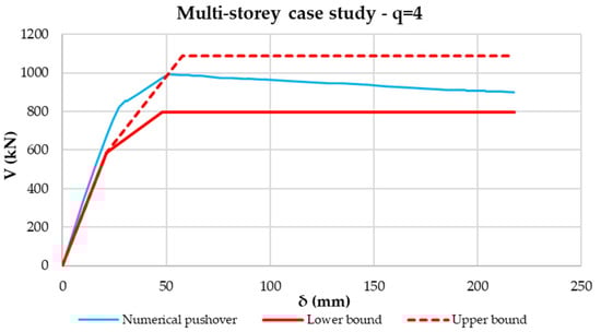
Figure 25.
Comparison between numerical pushover curve and analytical spindle for the multi-storey building case study with structure factor equal to 4.
7. Conclusions
In the paper, the elasto-plastic behavior of X-concentric braced steel frames with active tension diagonal bracings was analyzed. The construction of a pushover “spindle”, characterized by two trilinear analytical capacity curves, was defined. The proposal proved to be capable of grasping the real monotonic elasto-plastic behavior of the X-CBFs.
The main points developed in the work are listed below:
- It was first observed that the lateral stiffness of the X-CBFs in the Post-Buckling phase is not equal to half of the Pre-Buckling phase stiffness but is smaller and variable with the normalized slenderness of the diagonal.
- Taking these aspects into account, the construction of an analytical pushover “spindle” was proposed, characterized by lower- and upper-bound curves. Such limit curves form a field in which numerical pushover curves have to fall. This was proven by using a model validated through experimental tests. By varying the diagonal profiles with different normalized slenderness, it was shown that numerical curves fall always inside the proposed pushover spindle. In addition, the higher the normalized slenderness of the diagonal is, the tighter the analytical spindle is.
- The proposal was then extended to whole structures by analyzing mono- and multi-storey buildings. The numerical response of all the analyzed case studies falls back inside the spindle, which represents a strict strength domain and allows correctly evaluating the behavior of these types of structures.
- The proposed approach can be directly used in the design phase within the pushover method and allows a possible analytical control on the results obtained with the numerical model.
Author Contributions
Conceptualization, C.A. and L.B.; methodology, C.A. and L.B.; software, L.B.; validation, C.A., L.B. and S.N.; formal analysis, C.A. and L.B.; investigation, C.A. and L.B.; resources, C.A., L.B. and S.N.; data curation, L.B. and S.N.; writing—original draft preparation, L.B.; writing—review and editing, C.A., L.B. and S.N.; visualization, C.A., L.B. and S.N.; supervision, C.A., L.B. and S.N.; project administration, C.A., L.B. and S.N. All authors have read and agreed to the published version of the manuscript.
Funding
This research was funded by DPC-ReLUIS project 2019-2021 (WP12), Italy.
Data Availability Statement
The authors have all the data.
Conflicts of Interest
The authors declare no conflict of interest.
References
- British Standards Institution, European Committee for Standardization, British Standards Institution, and Standards Policy and Strategy Committee. Eurocode 8, Design of Structures for Earthquake Resistance; British Standards Institution: London, UK, 2005. [Google Scholar]
- American Institute of Steel Construction. Seismic Provisions for Structural Steel Buildings; American Institute of Steel Construction: Chicago, IL, USA, 2016. [Google Scholar]
- Goggins, J.; Salawdeh, S. Validation of nonlinear time history analysis models for single-storey concentrically braced frames using full-scale shake table tests. Earthq. Eng. Struct. Dyn. 2013, 42, 1151–1170. [Google Scholar] [CrossRef]
- Costanzo, S.; D’Aniello, M.; Landolfo, R. Proposal of design rules for ductile X-CBFS in the framework of EUROCODE 8. Earthq. Eng. Struct. Dyn. 2019, 48, 124–151. [Google Scholar] [CrossRef]
- Elghazouli, A.Y. Assessment of European seismic design procedures for steel framed structures. Bull. Earthq. Eng. 2010, 8, 65–89. [Google Scholar] [CrossRef]
- Costanzo, S.; Raffaele, L. Concentrically Braced Frames: European vs. North American Seismic Design Provisions. TOCIEJ Open Civ. Eng. J. 2017, 11, 453–463. [Google Scholar] [CrossRef][Green Version]
- D’Aniello, M.; Ambrosino, G.l.; Portioli, F.; Landolfo, R. Modelling aspects of the seismic response of steel concentric braced frames. Steel Compos. Struct. 2013, 15, 539–566. [Google Scholar] [CrossRef]
- Uang, C.-M.; Bruneau, M. State-of-the-Art Review on Seismic Design of Steel Structures. J. Struct. Eng. 2018, 144, 03118002. [Google Scholar] [CrossRef]
- Canadian Standards Association; Standards Council of Canada. Design of Steel Structures; Canadian Standards Association: Toronto, ON, Canada; Standards Council of Canada: Toronto, ON, Canada, 2019. [Google Scholar]
- Marino, E.M.; Nakashima, M.; Mosalam, K.M. Comparison of European and Japanese Seismic Design of Steel Building Structures. Eng. Struct. 2005, 27, 827–840. [Google Scholar] [CrossRef]
- Amadio, C.; Bomben, L.; Noè, S. Design of X-Concentric Braced Steel Frame Systems Using an Equivalent Stiffness in a Modal Elastic Analysis. Buildings 2022, 12, 359. [Google Scholar] [CrossRef]
- Wakabayashi, M.; Matsui, C.; Minami, K.; Mitani, I. Inelastic Behavior of Full-Scale Steel Frames with and without Bracings. Bull. Disaster Prev. Res. Inst. 1974, 24, 1–23. [Google Scholar]
- Black, R.G.; Wenger, W.A.; Popov, E.P. Inelastic Buckling of Steel Struts under Cyclic load Reversals; Report No. UCB/EERC-80/40; Earthquake Engineering Research Center: Berkeley, CA, USA, 1980. [Google Scholar]
- Kanyilmaz, A. Role of Compression Diagonals in Concentrically Braced Frames in Moderate Seismicity: A Full Scale Experimental Study. J Constr. Steel Res. 2017, 133, 1–18. [Google Scholar] [CrossRef]
- Zhao, B.; Zhou, T.; Chen, Z.; Yu, J. Experimental seismic behavior of SCFRT column chevron concentrically braced frames. J Constr. Steel Res. 2017, 133, 141–155. [Google Scholar] [CrossRef]
- Zhao, Z.; Liu, H.; Liang, B. Novel numerical method for the analysis of semi-rigid jointed lattice shell structures considering plasticity. ADES Adv. Eng. Softw. 2017, 114, 208–214. [Google Scholar] [CrossRef]
- Uriz, P.; Filippou, F.C.; Mahin, S.A. Model for Cyclic Inelastic Buckling of Steel Braces. J. Struct. Eng. 2008, 134, 619–628. [Google Scholar] [CrossRef]
- Applied Technology Council, United States, Federal Emergency Management Agency, and Building Seismic Safety Council (U.S.). NEHRP Guidelines for the Seismic Rehabilitation of Buildings; Applied Technology Council, United States, Federal Emergency Management Agency, and Building Seismic Safety Council (U.S.): Washington DC, USA, 1997. [Google Scholar]
- Faggiano, B.; Formisano, A.; Vaiano, G.; Mazzolani, F.M. Numerical Study on Concentric Braced X Frames under Monotonic and Cyclic Loads. Key Eng. Mater. 2018, 763, 633–641. [Google Scholar] [CrossRef]
- I. Computers and Structures. In SAP2000: Integrated Software for Structural Analysis and Design; CSI: Berkeley, CA, USA, 2006.
- Dicleli, M.; Calik, E.E. Physical Theory Hysteretic Model for Steel Braces. J. Struct. Eng. 2008, 134, 1215. [Google Scholar] [CrossRef]
- Ministero delle Infrastrutture e dei Trasporti, Italia. Norme Tecniche per le Costruzioni 2018: Decreto 17 Gennaio 2018 ‘Aggiornamento delle Norme Tecniche per le Costruzioni’; Ministero delle Infrastrutture e dei Trasporti, Italia: Rome, Italy, 2018.


Publisher’s Note: MDPI stays neutral with regard to jurisdictional claims in published maps and institutional affiliations. |
© 2022 by the authors. Licensee MDPI, Basel, Switzerland. This article is an open access article distributed under the terms and conditions of the Creative Commons Attribution (CC BY) license (https://creativecommons.org/licenses/by/4.0/).