Efficient Reliability Analysis of Structures Using Symbiotic Organisms Search-Based Active Learning Support Vector Machine

Abstract

Reliability-based design optimization considers the uncertainties that lie in the designing process of resilient buildings and structures. To model uncertainty, the major challenge is to lower the high computational expense incurred by the double-loop approach, where the design optimization (outer loop) repeatedly calls the reliability analysis of each structural design (inner loop). An alternative is to convert the reliability constraints to deterministic constraints by using optimality conditions. Yet, the approximated results are often inaccurate when constraint functions are highly non-linear, non-continuous, or non-differentiable. To achieve better accuracy while attaining sufficient flexibility, the present study proposes a new framework to classify the structural designs into feasible/infeasible designs. The proposed framework is called SOS-ASVM by integrating the symbiotic organism search (SOS) and the active-learning support vector machine (ASVM). ASVM is adopted as the surrogate model, while SOS is used to seek more representative samples to improve the classification accuracy of ASVM. The SOS-ASVM was validated by comparisons with popular classification tools: conventional support vector machine, artificial neural network, and Kriging model. Three practical engineering cases are used to demonstrate the performance of the SOS-ASVM: a cantilever beam, a bracket structure, and a 25-bar space truss. The comparison results confirm the superiority of the proposed framework to other tools.

1. Introduction

Structural design must comply with safety standards and minimize cost. Deterministic design optimization (DDO) is usually the preferred method for obtaining an optimal strategy. In DDO, the design variables and parameters are considered deterministic values. However, the structure is always affected by uncertainties in real-world applications, e.g., loading conditions, material properties, and manufacturing tolerances. DDO takes account of these uncertainties indirectly by using partial safety factors that are specified in design codes. Nonetheless, the solution may be close to the constraints because of this simplification, thereby increasing the probability of failure [1].

One method for addressing these problems is reliability-based design optimization (RBDO). RBDO is computationally expensive, and therefore, numerous studies have attempted to improve its efficiency. One approach to increase the computational efficiency of RBDO involves using a more efficient method to calculate structural reliability. The most probable point (MPP) concept is commonly used to calculate failure probability. However, MPP-based methods such as the first-order reliability method (FORM) and second-order reliability method (SORM) are suboptimal for practical and complex limit state functions [2]. Separately, Monte Carlo simulation (MCS) and other simulation methods are commonly used to estimate failure probability. In contrast to MPP-based methods, MCSs do not depend on the shape of the limit state function, but they require extensive computation to simulate a low-probability event [3].

Alternatively, subset simulation (SS), a relatively new method, estimates failure probability by using a sequence of conditional failure probabilities [4]. This method addresses the computational inefficiency of MCSs in handling small failure probability events. However, the precision of a result is sensitive to the parameters that govern the intermediate failure levels [5]. Another approach to increase the efficiency of RBDO involves modifying the integration of reliability analysis and design optimization. 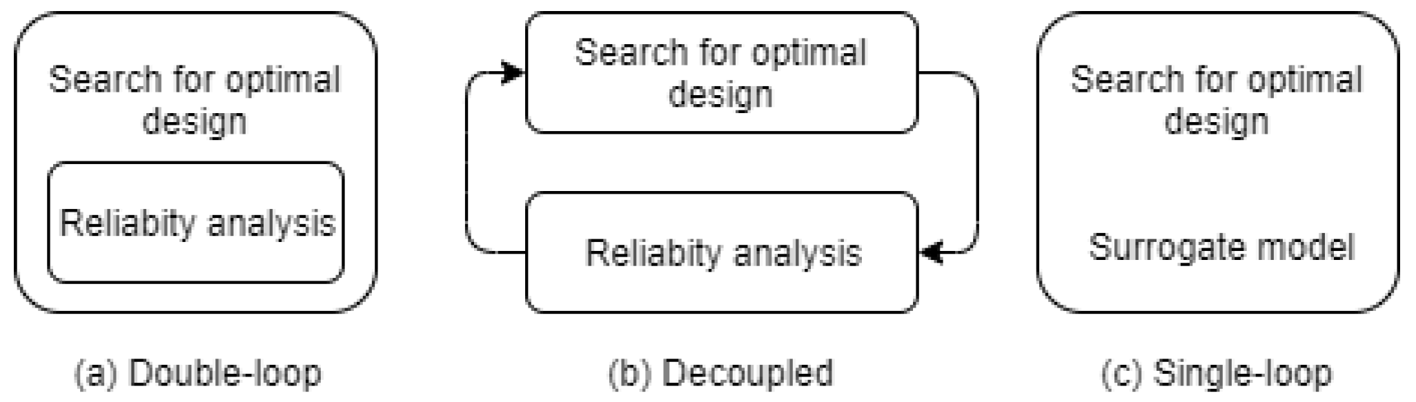Three methods for solving this problem have been reported: double-loop [6,7,8,9,10], single-loop [11,12,13,14,15], and decoupled methods [16,17,18,19,20], shown in Figure 1. The double-loop method uses two nested loops, with the outer and inner loops performing optimization and reliability evaluation, respectively. This means that every optimization candidate must be subjected to a computationally expensive reliability analysis, which increases the computational cost of this method. In the single-loop method, the computationally expensive reliability analysis is replaced with an approximation function or surrogate model. The decoupled method attempts to decouple the two loops into a series of single loops by employing a specific strategy and solving the loops sequentially until a particular stopping condition, for which some convergence criteria are usually specified, is fulfilled [21]. Although the single-loop and decoupled methods significantly increase the efficiency of solving the RBDO problem, they do not necessarily guarantee convergence to a stable result [22]. Both methods introduce a tradeoff between accuracy and efficiency.

As mentioned, the single-loop method increases the computational efficiency of RBDO by using a computationally cheaper surrogate model in place of the computationally expensive reliability analysis. A variety of surrogate models have been proposed for this purpose, such as the artificial neural network (ANN) [23], support vector machine (SVM) [24], response surface method (RSM) [25], and Kriging interpolation [26]. Various surrogate-based RDBO techniques have been developed in recent years to lessen the computation burden of performing reliability analysis. Liu et al. [27] proposed to use a new RBDO framework where the cooperation of SVM and Kriging is used to find the optimum design point. Hawchar et al. [28] presented a Kriging-based model that addresses the time-variant RBDO problems. Zhou and Lu [29] investigated the application of sparse polynomial chaos expansion which is complemented with an active learning technique. Shang et al. [30] combined radial basis function with sparse polynomial chaos expansion to enhance the capability of model prediction. Fan et al. [31] performed reliability-based design optimization on crane system designs which are modeled using the Kriging model.

To achieve a high level of accuracy while maintaining adequate flexibility, in the present study, we propose a new framework to classify structural designs into feasible/infeasible designs without running a time-consuming reliability analysis. The proposed framework, called SOS-ASVM, integrates symbiotic organisms search (SOS), an active-learning support vector machine (ASVM), and MCS. SOS is a new and powerful metaheuristic algorithm that simulates the symbiotic interaction strategies used by organisms to survive in an ecosystem. The main advantage of using SOS is that it does not require a tuning parameter [32]. In the preliminary research, several well-known optimizers such as genetic algorithm (GA) and particle swarm optimization (PSO) were examined. We found that SOS gives the best performance out of the investigated optimization techniques. We used an SVM because it has good learning capacity and generalization capability, even with a small sample set [33]. In addition, we developed an active-learning strategy to boost the efficiency of the SVM model. This strategy improves accuracy by actively selecting the most informative samples rather than randomly picking samples. The classification of the training samples is performed by MCS according to the pre-specified failure probability threshold.

The remainder of this paper is organized as follows. In Section 2, we define and explain the RBDO problem. Section 3 explains the methodology of the SOS-ASVM and each of its components in detail. In Section 4, we provide several examples to verify the performance of the SOS-ASVM. Our concluding remarks are given in Section 5.

2. Reliability-Based Design Optimization

In RBDO, the variables contributing to a structure’s performance can be divided into two types: design variables and random variables. Design variables represent the elements of a structure that may be picked from continuous or discrete selections. Random variables are used to account for the uncertainties that exist in the material and the loading condition of the structure.

The RBDO problem can be formulated as follows:

$$\begin{gathered} \underset{\mathit{X}}{\min }C\left(\mathit{X},\mathit{R}\right) \\ \mathrm{s}.\mathrm{t}. P_f\left(\mathit{X},\mathit{R}\right)\le \overline{P_f} \end{gathered}$$

(1)

where $C\left(\mathit{X},\mathit{R}\right)$ is the cost function, which includes the material cost or structural weight, $\mathit{X}$ denotes the design variables, $\mathit{R}$ denotes the random variables, $P_f\left(\mathit{X},\mathit{R}\right)$ is the system failure probability function, and $\overline{P_f}$ is the specified failure probability threshold.

In RBDO, the selection of design variables is considered infeasible when the failure probability of the system exceeds a specified threshold. Finding the failure probability of a design is a time-consuming process, and given a considerable number of design combinations for optimization, it is vital to find a more efficient method to replace reliability analysis. We thus developed a framework to replace the time-consuming reliability analyses used to determine the feasibility of a design.

3. The SOS-ASVM Framework

The proposed SOS-ASVM framework consists of three components: SOS, ASVM, and MCS. SOS and the ASVM are described later, followed by a complete explanation of the SOS-ASVM framework.

3.1. Symbiotic Organisms Search

SOS is a simple and powerful metaheuristic that employs a population-based search strategy to identify the optimal solution for a given objective function.

Similar to other population-based metaheuristic algorithms, SOS begins with an initial population called the ecosystem. In the ecosystem, a group of organisms is generated randomly in the search space. In the next step, a new generation consisting of new organisms is generated by imitating the biological interactions between two organisms in an ecosystem. The following three phases that resemble the real-world biological interaction model are used in SOS: mutualism, commensalism, and parasitism. Each organism interacts with the other organisms randomly in all of these phases. The process is repeated until the termination condition is fulfilled. The entirety of this procedure is summarized in Figure 2.

3.1.1. Mutualism Phase

The mutualism phase simulates mutualistic interactions that benefit both participants. An example of such interactions is evident in the relationship between bees and flowers. Bees benefit by gathering nectar and pollen from flowers. Flowers benefit because the pollination performed by the bees helps the flowers to reproduce.

In the mutualism phase, organism X_i is matched randomly with organism X_j. The new candidate solutions are then calculated based on the mutualistic relationship modeled using Equations (2) and (3).

$$X_{inew}=X_i+rand\left(0, 1\right)\left(X_{best}-MV\times B{F}_1\right)$$

(2)

$$X_{jnew}=X_j+rand\left(0, 1\right)\left(X_{best}-MV\times B{F}_2\right)$$

(3)

$$MV=\frac{X_i+X_j}{2}$$

(4)

Here, the benefit factors BF₁ and BF₂ are determined randomly as either 1 or 2. These factors simulate whether an organism partially or fully benefits from an interaction. X_best represents the best organism within the current ecosystem, and rand (0, 1) is a uniformly distributed random number between 0 and 1.

3.1.2. Commensalism Phase

The commensalism phase simulates a commensalistic relationship in which one participant is benefitted and the other is generally unaffected. An example of such a relationship is that between sharks and remora fish. The remora attaches itself to the shark and benefits by eating the scraps of food left by the shark. The shark is unaffected by the remora’s activities and receives almost no benefit from the relationship.

Similar to the mutualism phase, in the commensalism phase, two organisms are randomly selected. However, in this scenario, only organism X_i benefits from the interaction. The new candidate solution is then calculated using Equation (5):

$$X_{inew}=X_i+rand\left(-1, 1\right)\left(X_{best}-X_j\right)$$

(5)

where X_best represents the best organism within the current ecosystem, and rand (−1, 1) is a uniformly distributed random number between −1 and 1.

3.1.3. Parasitism Phase

The parasitism phase simulates parasitic interactions in which one participant is benefitted and the other is harmed. An example of such a relationship is that between a mosquito and its host. The mosquito benefits by feeding on its host’s blood, whereas the host may be harmed by receiving a deadly disease caused by a pathogen the mosquito carries.

In SOS, organism X_i is modeled similar to the Anopheles mosquito. Organism X_i creates an artificial parasite by copying and mutating itself. Then, the parasite is matched randomly with organism X_j, which serves as the host to the newly created parasite. If the parasite has a greater fitness value than the host, it replaces the position of organism X_j in the ecosystem. However, if the fitness value of organism X_j is superior to that of the parasite, the parasite is removed from the ecosystem.

3.2. Support Vector Machine

An SVM is a highly efficient machine learning technique that has been used in many applications and fields for its classification and pattern-recognition abilities. Fundamentally, an SVM uses training data samples to construct a hyperplane that can separate a given set of data samples into their respective categories. This section provides a brief overview of SVMs; a more comprehensive account can be referred to [34].

In the present study, an SVM is used to replace the time-consuming reliability analysis. To this end, the SVM is used to develop a hyperplane that can predict the feasibility of each design parameter vector based on the failure probability computed by means of MCS. In this case, each vector is assigned a label that indicates its feasibility.

Consider a two-class problem. A set of N training samples, X_i with d-dimensional space, and the label indicator y_i with a value of either 1 or −1, as illustrated in Figure 3, are used as the training samples to build a separating hyperplane. The SVM finds the most optimal manner in which to assign each training sample to two data classes. The optimal hyperplane is defined as having the maximum margin. The linear function of the hyperplane can be formulated as follows:

$$\mathit{w}·\mathit{X}+b=0$$

(6)

where w is the normal vector of the hyperplane and b is the bias parameter. All the training samples should satisfy the following constraints:

$$y_i\left(\mathit{w}·{\mathit{X}}_i+b\right)-1\ge 0$$

(7)

This constraint ensures that no sample is within the margin. The margin width can be defined as $\raisebox{1ex}{$2$}\!\left/ \!\raisebox{-1ex}{$\left|\right|\mathit{w}\left|\right|$}\right.$. Therefore, the determination of the optimal parameter w, b can be formulated as the following optimization problem:

$$\begin{gathered} \underset{\mathit{w},b}{\min }\frac{{\left|\right|\mathit{w}\left|\right|}^2}{2} \\ \mathrm{s}.\mathrm{t}. y_i\left(\mathit{w}·{\mathit{X}}_i+b\right)-1\ge 0, i=1, \dots , N \end{gathered}$$

(8)

When the data are not linearly separable, the SVM is extended to deal with this problem by using the soft margin method. The inequality constraint is relaxed by introducing a slack variable ${\xi }_i$ that penalizes each misclassification in the training dataset. The original problem is then transformed into the following Equation (9):

$$\begin{gathered} \underset{\mathit{w},b}{\min }\frac{{\left|\right|\mathit{w}\left|\right|}^2}{2}+\mathrm{C}{\displaystyle \sum }_{i=1}^N{\xi }_i \\ \mathrm{s}.\mathrm{t}. y_i\left(\mathit{w}·{\mathit{X}}_i+b\right)-1\ge -{\xi }_i, i=1, \dots , N \end{gathered}$$

(9)

where C is a regularization parameter. The parameter C in the soft margin method permits misclassification, and stricter separation between classes can be achieved by increasing the value of C.

The optimization problem given in Equations (8) and (9) is a quadratic programming (QP) problem, and it can be solved using the existing optimization solvers. The results obtained include the optimal w, b, and the Lagrange multiplier ${\alpha }_i$. The nonzero Lagrange multiplier exists only at the points closest to the hyperplane. Thus, only the points that contribute to the construction of the SVM hyperplane are called support vectors. A new arbitrary point X can be classified using the following Equation (10):

$$y\left(\mathit{X}\right)=sign\left[{\displaystyle \sum }_{i=1}^{NSV}{\alpha }_i{y}_i{\mathit{X}}_i{}^T\mathit{X}+b\right]$$

(10)

where NSV is the number of support vectors, which represents a small fraction of the total number of training samples.

The SVM can also be extended to non-linear cases in which the samples cannot be separated using the linear hyperplane. The main idea is to project the data points onto a higher-dimensional space (feature space) where they can be separated linearly. A kernel function is used to execute the transformation required to solve this problem. Many types of kernel function are available, and the Gaussian kernel used in this paper is defined as:

$$K\left({\mathit{X}}_i,\mathit{X}\right)=\exp \left(-\frac{{\left|\right|{\mathit{X}}_i-\mathit{X}\left|\right|}^2}{2{\sigma }^2}\right)$$

(11)

where $\sigma$ is the adjustable width parameter of the Gaussian kernel. With the addition of the kernel function to the SVM, Equation (10) for the classification of a new arbitrary point X can be rewritten as:

$$y\left(\mathit{X}\right)=sign\left[{\displaystyle \sum }_{i=1}^{NSV}{\alpha }_i{y}_{i}K\left({\mathit{X}}_i,\mathit{X}\right)+b\right]$$

(12)

Notably, the effectiveness of the SVM strongly depends on the selection of its hyper-parameters.

3.3. Active-Learning Support Vector Machine

The primary difference between an active learner and a passive learner is in how they enrich the training set. The active learner enriches its training set by actively picking the most informative samples to improve the model’s performance continuously. On the other hand, the passive learner enriches its training set randomly. Therefore, the active learner can outperform its counterpart in terms of efficiency because it can build the model with as few training samples as possible. The active learning for classification was proposed by Lewis and Gale [35] for text classification purposes. Lewis and Gale [35] propose that the samples used for training should be the samples with the highest probability of being misclassified. Song et al. [36] proposed an active-learning SVM (ASVM) for calculating the failure probability. In that framework, the new samples are chosen from the candidate samples within the margin with the maximum distance to the nearest existing training sample. Pan and Dias [37] proposed an active learning scheme similar to the scheme developed by Song, Choi, Lee, Zhao, and Lamb [36]. However, the learning function is modified to find the sample closest to the SVM boundary, which need not be inside the margin and have the maximum distance from its nearest existing training sample.

4. SOS-ASVM Framework

In this section, the proposed integrated SOS-ASVM framework is introduced. In this framework, to continuously improve the SVM model, the concept of an active-learning strategy is implemented in the SVM to actively select samples instead of randomly selecting training samples. This active-learning strategy has been shown to be more efficient than its passive counterpart [37]. The main concept behind the ASVM is the inclusion of training samples that contain the most information about and have the most substantial influence on the shape of the hyperplane. In this regard, the samples near the hyperplane, as opposed to those relatively far from the hyperplane, gain importance because the SVM hyperplane is influenced only by its support vectors. The density of the next set of training samples can also be considered in the ASVM because a sparse area holds more new information than a densely sampled area does. To further increase the efficiency of the framework, SOS is used to efficiently navigate through the search space to identify the best sample based on these criteria. The interaction between the components of the SOS-ASVM is illustrated in Figure 4.

A flowchart describing the integrated SOS-ASVM framework is depicted in Figure 5. The entire process of the proposed framework comprises the following steps:

1.

Generate the initial training samples. The initial training samples should contain samples from both classes because the ASVM uses the available information to select the next sample. To capture the overall behavior of the search space, we used the Latin hypercube design (LHD) to enforce uniformity in the samples. The initial samples should subsequently be evaluated using MCS to determine the feasibility of the design through comparison with the predetermined threshold. According to our experiment, the suggested number of initial training samples is 20–50 samples depending on the complexity of the problem. The process of generating the initial samples is illustrated in Figure 6a.

2.

Construct the SVM model based on the current training samples. The construction of the SVM hyperplane is illustrated in Figure 6b.

3.

SOS is employed to find the next sample for enriching the current SVM model. As stated earlier in regards to the ASVM, the best sample to add to the model is the one with the most information and the strongest influence on the model. Therefore, to find the next sample, SOS is used to find the sample closest to the hyperplane and the farthest from the current training samples. The objective function of SOS can be formulated as follows:

$$f\left(\mathit{X}\right)=\underset{\mathit{X}}{\min }\frac{s\left(\mathit{X}\right)}{d\left(\mathit{X}\right)}$$

(13)

$$s\left(\mathit{X}\right)=abs\left({\displaystyle \sum }_{i=1}^{NSV}{\alpha }_i{y}_{i}K\left({\mathit{X}}_i,\mathit{X}\right)+b\right)$$

(14)

$$d\left(\mathit{X}\right)=\left|\right|\mathit{X}-{\mathit{X}}_{nearest}\left|\right|$$

(15)

where $s\left(\mathit{X}\right)$ is a function that calculates the representative distance between point $\mathit{X}$ and the SVM hyperplane, and $d\left(\mathit{X}\right)$ is the distance function for calculating the distance between point $\mathit{X}$ and the nearest sample within the current training samples (${\mathit{X}}_{nearest}$). After the best candidate is identified, the sample is evaluated using MCS and classified according to its feasibility. The process of finding the next optimal sample by using SOS is illustrated in Figure 6c.

4.

Enrich and reconstruct the SVM model with optimization of the hyperparameter after every nth iteration. The samples obtained in the previous step are added to the pool of training samples to update the SVM model. To improve the efficiency of the framework, the hyperparameter is updated after every nth addition of new samples. In this paper, the variable n is set to 2, but it can be adjusted to improve either the effectiveness or efficiency of the framework. The process of reconstructing the SVM hyperplane is illustrated in Figure 6d.

5.

The SOS-ASVM framework is terminated when the stopping condition is fulfilled. The stopping conditions, such as the maximum number of iterations, and convergence limit, can be defined by the user. If the stopping condition is not achieved, the framework returns to Step 3.

Notably, the SOS-ASVM is proposed herein to improve the traditional surrogate-based reliability analyses, which deliver less satisfactory results when faced with a more complex limit state function, such as discontinuous or non-linear limit state functions. Moreover, throughout the process of the proposed framework, the time-consuming MCS is used only to evaluate the training samples. In step 3, the framework uses the classification ability of the SVM model instead, which is computationally less expensive.

5. Case Study

The performance of the proposed SOS-ASVM framework was tested on three practical structural examples, namely, a cantilever beam, a bracket structure, and a 25-bar space truss. A feasibility constraint was set for each problem to ensure that the probability of failure did not exceed 1 × 10⁻³:

$$P(G\left(\mathit{X}, \mathit{R}\right)<0)\le 1\times {10}^{-3}$$

(16)

For each of the problems, the results obtained using the SOS-ASVM were compared with those obtained with traditional surrogate models that use SVM, ANN, and Kriging models. To this end, the classification accuracies of these models on randomly generated test samples were compared.

5.1. Experimental Setup

To make a fair comparison, all the models start with the same group of random samples called the “training” dataset. In every iteration, all the models except for the SOS-ASVM pick a random sample that is added to the “training” dataset. The “training” dataset is used to train each surrogate model. In contrast, the SOS-ASVM will actively pick the best sample to add to the “training” dataset instead of a random sample. The models are then tested on the “test” dataset to distinguish the samples between two classes (feasible or infeasible). In this study, the “test” dataset contains 10⁵ randomly generated samples. The “training” and “test” datasets are generated by sampling the combinations of design variables according to their individual distributions. The classification error is calculated by the Equation below:

$$err=\frac{n_{miss}}{n_{total}}\times 100\%$$

(17)

where n_miss is the number of misclassified samples in the “test” dataset and n_total is the total number of samples in the “test” dataset.

The improvement of each surrogate model is calculated to show the level of improvement the current model achieved compared with the worst one among the SVM, ANN, and Kriging models. The improvement is calculated by the equation below:

$$imp=\frac{\left|err-er{r}_{worst}\right|}{er{r}_{worst}}\times 100\%$$

(18)

where err is the classification error of the current model and err_worst is the classification error of the worst performing model. For example, if the worst model yields 20% error and the current model yields 10% the improvement will be $\frac{\left|10\% - 20\%\right|}{20\%} \times 100\%=50\%$. Since the metaheuristic algorithm has an inherent stochastic property, multiple runs of SOS-ASVM have been considered.

5.2. Parameter Selection

The present SOS-ASVM adopts the Gaussian kernel according to preliminary runs. The C parameter is set to be infinite to enforce a strict hyperplane and give the model more stability. Lastly, the remaining γ parameter will be determined using 5-fold cross-validation.

The SOS-ASVM is compared with several popular surrogate models: SVM, ANN, and Kriging models. The parameters of these models are set as follows. For SVM, the hyper-parameter was tuned using the same treatment as that for the proposed framework, which involved the five-fold crossover method. A multilayer feedforward backpropagation network, one of the most well-known and widely used ANN paradigms [38], was selected as the ANN architecture. The said ANN structure consisted of an input layer, a hidden layer, and an output layer. The process for the selection of the optimal number of neurons within the hidden layer is up for debate because there are no general rules for selecting the correct number. Therefore, in this study, we selected (2n + 1) neurons for the hidden layer, where n denotes the number of neurons in the input layer [39]. A logistic transfer function is used to transfer the values of the input layer nodes to the hidden layer nodes, whereas a linear transfer function is adopted to transfer the values from the hidden layer to the output layer. Lastly, for the Kriging model, ordinary Kriging and the Gaussian correlation function were adopted in this paper.

5.3. Cantilever Beam

The first example was a simple cantilever beam under point load [40], as illustrated in Figure 7. The assumed normally distributed random variables of the cantilever beam were as follows: concentrated load (P) = N(20, 1.2) kN, beam length (L) = N(400, 1.0) mm, and strength of material (R) = N(200, 10) MPa. The design variables, including beam width (B) and beam depth (H), were selected from a continuous value with a maximum of 100 mm. The probability of failure for this problem was formulated as follows:

$$P_f=P(G\left(\mathit{X}, \mathit{R}\right)<0)=P\left(R-\frac{6PL}{B{H}^2}<0\right)$$

(19)

The performance of the SOS-ASVM is compared with other popular surrogate modeling methods in terms of classification accuracy and computational effort. The best result achieved for each method using 200 samples can be seen in

Table 1. Best classification accuracy achieved for cantilever beam.

Method	Avg. err (%)	Std. err	imp (%)
SOS-ASVM	0.220	0.011	89.460
ANN	2.087	-	-
Kriging	1.423	-	31.833
SVM	0.758	-	63.666

. The classification error of the proposed SOS-ASVM framework is merely 0.22%, the lowest among the four methods. The error of the SOS-ASVM yields an average of 89.460% improvement over the classification error of ANN—the worst one among all four methods. The whole process took SOS-ASVM about 2.968 h to complete.

Figure 8 compares the classification errors of four methods as the number of training samples increases. The proposed SOS-ASVM framework can achieve much lower classification error and convergence quicker compared with the other models. It can be observed that the classification error of ANN fluctuates significantly without any sign of convergence. The performance of SVM and Kriging is pretty similar in terms of the convergence speed but with much better accuracy. Note that oscillation in the classification error is to be expected because the addition of an extra sample may not always improve the accuracy. However, increasing the number of training samples would gradually lead to better accuracy.

5.4. Bracket Structure

The next case is a bracket structure [41] shown in Figure 9. The bracket structure is loaded with concentrated load (P) on the right tips and its own weight due to gravity (g). The design and random variables are presented in

Table 2. Characteristics of random variables for bracket structure.

Random Variables	Description	Distribution	Mean Value	c.o.v
P	Load (kN)	Gumbel	100	0.15
E	Young’s modulus (GPa)	Gumbel	200	0.08
fy	Yielding stress (GPa)	Normal	0.225	0.08
ρ	Density (kg/m3)	Normal	7860	0.1
L	Length (m)	Normal	5	0.05
wAB	Width of beam AB (m)	Normal	0.1–0.3	0.05
wCD	Width of beam CD (m)	Normal	0.1–0.3	0.05
t	Height of beam (m)	Normal	0.1–0.3	0.05

. There are two failure events considered for this problem: maximum stress and buckling. The system fails when either one of the failure events occurs.

The maximum stress (${\sigma }_{max}$) should not exceed the yielding stress of the material ($f_y$). The failure event can be formulated as follows:

$$G_1\left(\mathit{X},\mathit{Z}\right)=f_y-{\sigma }_{max}$$

(20)

where:

$${\sigma }_{max}=\frac{6M_B}{w_{CD}{t}^2}$$

(21)

$$M_B=\frac{PL}{3}+\frac{\rho g{w}_{CD}t{L}^2}{18}$$

(22)

The second failure event considers the buckling effect where the maximum axial load ($F_{max}$) in each member should not exceed the Euler critical buckling load ($F_{buckling}$) (neglecting its own weight). Therefore, the second limit state function can be expressed as:

$$G_2\left(\mathit{X},\mathit{Z}\right)=F_{buckling}-F_{max}$$

(23)

where:

$$F_{buckling}=\frac{{\pi }^{2}EI}{L_{AB}{}^2}=\frac{{\pi }^{2}Et{w}_{AB}{}^{3}9{\sin }^2\theta }{48L^2}$$

(24)

$$F_{max}=\frac{1}{\cos \theta }\left(\frac{3P}{2}+\frac{3\rho g{w}_{CD}tL}{4}\right)$$

(25)

The proposed SOS-ASVM framework is compared with other popular surrogate models. The best result achieved for each method is listed in

Table 3. Best classification accuracy achieved for bracket structure.

Method	Avg. err (%)	Std. err	imp (%)
SOS-ASVM	2.011	0.032	65.948
ANN	3.067	-	48.062
Kriging	5.906	-	-
SVM	2.108	-	64.310

. Here, the SOS-ASVM achieved a classification error of 2.01%, which is significantly better than all the other models. The Kriging model has the worst performance as the classification error is the highest, 5.906%. Compared with the Kriging method (the worst of the four methods), the SOS-ASVM yields over 65.9% improvement in terms of classification error. The whole process took SOS-ASVM about 3.459 h to complete.

Figure 10 shows the classification error of each method as a function of the number of training samples used. Observe that the classification error of ANN fluctuates significantly and possesses no sign of convergence. The best classification error of the SOS-ASVM and SVM in Table 3 is quite close; however, as seen in Figure 10, the proposed SOS-ASVM framework converged much faster. Fast convergence is particularly desirable when dealing with time-consuming reliability analysis, as it reduces the number of samples needed to train the model.

5.5. 25-Bar Space Truss

The performance of the proposed SOS-ASVM framework was verified by applying it to the 25-bar space truss problem [42], as illustrated in Figure 11. The truss members were selected from the 72 choices of standard-sized hollow pipe listed in

Table 4. Choice of design variable.

Bar No.	D (mm)	T (mm)	A (mm2)	Bar No.	D (mm)	T (mm)	A (mm2)
1	21.7	2	123.8	37	216.3	7	4602.7
2	27.2	2	158.3	38	216.3	8	5235.2
3	27.2	2.3	179.9	39	216.3	8.2	5360.9
4	34	2.3	229.1	40	267.4	6	4927.3
5	42.7	2.3	291.9	41	267.4	6.6	5407.6
6	42.7	2.5	315.7	42	267.4	7	5726.5
7	48.6	2.3	334.5	43	267.4	8	6519.4
8	48.6	2.5	362.1	44	267.4	9	7306.1
9	48.6	2.8	402.9	45	267.4	9.3	7540.9
10	48.6	3.2	456.4	46	318.5	6	5890.5
11	60.5	2.3	420.5	47	318.5	6.9	6754.6
12	60.5	3.2	576	48	318.5	8	7803.7
13	60.5	4	710	49	318.5	9	8750.9
14	76.3	2.8	646.5	50	318.5	10.31	9982.2
15	76.3	3.2	734.9	51	355.6	6.4	7021.1
16	76.3	4	908.5	52	355.6	7.9	8629.4
17	89.1	2.8	759.1	53	355.6	9	9799.9
18	89.1	3.2	863.6	54	355.6	9.5	10,329.4
19	101.6	3.2	989.2	55	355.6	12	12,953.4
20	101.6	4	1226.5	56	406.4	7.9	9890.2
21	101.6	5	1517.4	57	406.4	9	11,236.2
22	114.3	3.2	1116.9	58	406.4	9.5	11,845.5
23	114.3	3.5	1218.3	59	406.4	12	14,868.5
24	114.3	4.5	1552.3	60	406.4	12.7	15,707.9
25	114.3	5.6	1912.4	61	406.4	16	19,623.6
26	139.8	3.6	1540.4	62	457.2	9	12,672.6
27	139.8	4	1706.5	63	457.2	9.5	13,361.7
28	139.8	4.5	1912.8	64	457.2	12	16,783.6
29	139.8	6	2522.1	65	457.2	12.7	17,734.8
30	165.2	4.5	2271.8	66	457.2	16	22,177.1
31	165.2	5	2516.4	67	508	7.9	12,411.8
32	165.2	6	3000.8	68	508	9	14,108.9
33	165.2	7.1	3526.5	69	508	9.5	14,877.8
34	216.3	4.5	2994.3	70	508	12	18,698.8
35	216.3	5.8	3835.6	71	508	12.7	19,761.6
36	216.3	6	3964.1	72	508	14	21,727.3

, which also lists the outside diameter (D), thickness (t), and area (A) of these pipes. The truss was subjected to two normal loads under condition 1 and two loads with an uncertain component under condition 2, as summarized in

Table 5. Load conditions for 25-bar problem.

Joints	Condition 1 (in kN)			Condition 2 (in kN)
	Px	Py	Pz	Px	Py	Pz
1	100	−1000	−1000	0	0	0
2	0	−1000	−1000	0	0	0
3	0	0	0	P1	0	0
6	0	0	0	P2	0	0

. The modulus of elasticity (E) was set to 2 × 10⁵ N/mm². The 25 bars were divided into six groups, where the same hollow bar was assigned to the members of the same group. The grouping in this problem, summarized in

Table 6. Grouping of bars for 25-bar problem.

Group	Bar ID
1	1
2	2, 3, 4, 5
3	6, 7, 8, 9
4	10, 11, 12, 13
5	14, 15, 16, 17, 18, 19, 20, 21
6	22, 23, 24, 25

, was intended to ease the connection between the truss bars and minimize errors during construction. The following random variables were used in this problem: loads P₁ and P₂, cross-sectional areas A₁–A₆, and yield stresses F_y1–F_y25. Details of the properties of these random variables are listed in

Table 7. Characteristics of random variables for 25-bar problem.

Random Variables	Distribution	Mean Value	Dispersion
P1, P2	Extreme type I	500 kN	c.o.v. = 5%
A1–A6	Uniform	Selection from Table 4	±5%
Fy1–Fy25	Lognormal	μ = 0.250 GPa	c.o.v. = 5%

.

In this problem, a failure event was defined as occurring when one or more truss components exceeded the allowable/yield stress, and it is expressed as the following equation:

$$\left|{\sigma }_i\right|>F_y$$

(26)

where σ_i denotes the axial stress of the i-th member in the structure, and F_y is the yield stress.

The effect of buckling on compressed members was also considered to be one of the failure conditions of the structure. Buckling refers to a sudden change in the shape of a structural component under compression. This deformation may cause complete loss of the member’s load-carrying capacity and eventually lead to failure (collapse) of the entire system. The critical buckling yield stress is modeled as Equations (27) and (28):

$$F_{cr}=({0.658}^{{\mathsf{\lambda }}_c^2})F_y \left({\mathsf{\lambda }}_c\le 1.5\right)$$

(27)

$$F_{cr}=\left(\frac{0.877}{{\mathsf{\lambda }}_c^2}\right)F_y ({\mathsf{\lambda }}_c>1.5)$$

(28)

where $F_{cr}$ denotes the critical buckling stress, and ${\mathsf{\lambda }}_c$ denotes the slenderness ratio that can be calculated using Equation (29):

$${\mathsf{\lambda }}_c=\frac{KL}{\mathsf{\pi }\mathrm{r}}\sqrt{\frac{F_y}{E}}$$

(29)

$$r=\sqrt{\frac{I}{A}}$$

(30)

where K is the effective length factor, L the unbraced length, r the radius of gyration, and E the modulus of elasticity. The radius of gyration is calculated using Equation (30), where I denotes the area moment of inertia, and A denotes the cross-sectional area of the member.

Like the previous examples, the SOS-ASVM is compared with other popular surrogate models in terms of classification accuracy and computational effort. The best result achieved by each respective method is listed in

Table 8. Best classification accuracy achieved for 25-bar space truss.

Method	Avg. err (%)	Std err.	imp (%)
SOS-ASVM	3.887	0.108	52.135
ANN	7.267	-	10.513
Kriging	8.121	-	0
SVM	6.017	-	25.911

. The performance of the SOS-ASVM is substantially better than the other models; it achieves a low classification error of 3.887%, representing 52.135% improvement in contrast to Kriging. The whole process took SOS-ASVM about 2.954 h to complete.

Figure 12 shows the classification error yielded by all the methods as a function of the number of samples. As seen in Figure 12, the SOS-ASVM outperforms the other methods in terms of classification error and convergence speed. This problem addresses many practical issues, such as multiple failure conditions, non-linear limit state function, and discontinuous design variables. It highlights the advantage of the SOS-ASVM in practical situations, where the other surrogate modeling methods are less than satisfactory.

5.6. Summary

Table 9. Performance ranking of all methods.

Method		SOS-ASVM	SVM	ANN	Kriging
Case 1	err (%)	0.220	0.758	2.087	1.423
	Rank	1	2	4	3
Case 2	err (%)	2.011	2.108	3.067	5.906
	Rank	1	2	3	4
Case 3	err (%)	3.887	7.267	8.121	6.017
	Rank	1	3	4	2
Total rank		3	10	11	6
Overall ranking		1	3	4	2

summarizes the performance of all four methods. For each case, individual methods are ranked based on their classification error. The overall ranking is determined using the total rank obtained by summing all the ranks of each case study. The total rank is arranged in ascending order: the method with the lowest total rank is determined as the best method. In all three cases, the SOS-ASVM always obtains the best classification error compared with the other surrogate models. It highlights that the SOS-ASVM is more consistent than all the other surrogate modeling methods: ANN, SVM, and Kriging.

6. Conclusions

A new framework called SOS-ASVM that combines three components—SOS, ASVM, and MCS—into one cohesive framework is introduced in this paper. This framework was developed to improve the accuracy and efficiency of surrogate-based models to replace the time-consuming process of reliability analysis. For the proposed framework, the concept of ASVM is adopted to actively select samples and improve model performance. SOS is employed to efficiently navigate the search space to find the best samples, which are then evaluated using MCS before being incorporated into the model.

The proposed SOS-ASVM framework was applied to three practical problems: a cantilever beam, a bracket structure, and a 25-bar space truss. The results were used to compare the SOS-ASVM with traditional surrogate-based models such as the SVM, ANN, and Kriging methods. It is found that the proposed SOS-ASVM framework is more effective and efficient in classifying the feasibility of the design solutions in all the cases. The SOS-ASVM provides much lower classification error: 0.22% in cantilever beam, 2.01% in bracket structure, and 3.89% in 25-bar space truss, compared with the other methods. The comparison results indicated that in all of the presented examples, the proposed SOS-ASVM framework was more effective and efficient for modeling the feasibility of a design. The difference between the SOS-ASVM and the other methods is more pronounced in the last example, the 25-bar space truss, where the SOS-ASVM achieved 3.89% classification error compared with SVM (6.02%), ANN (7.27%), and Kriging (8.12%). This indicates that the proposed SOS-ASVM framework is more attractive when the problem complexity is higher.