
Leakage Diagnosis of Air Conditioning Water System Networks Based on an Improved BP Neural Network Algorithm


Abstract
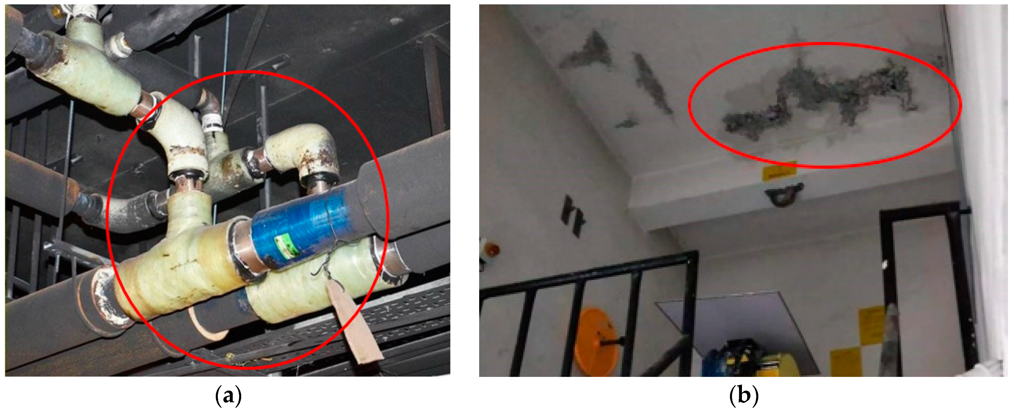
:1. Introduction
2. Materials and Methods
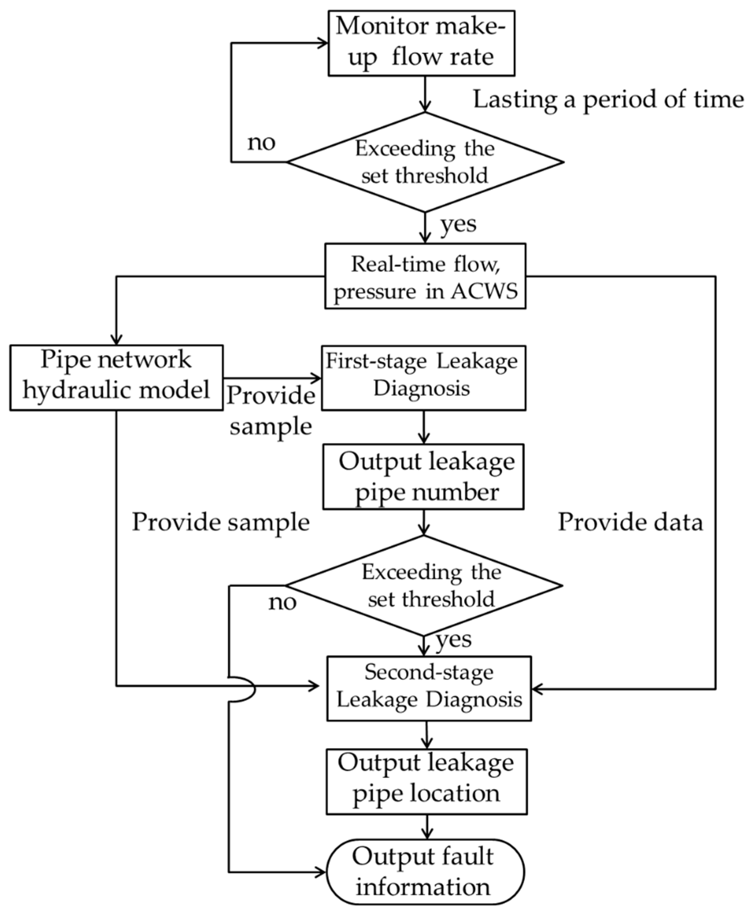
2.1. Research Overview
2.2. Method Description
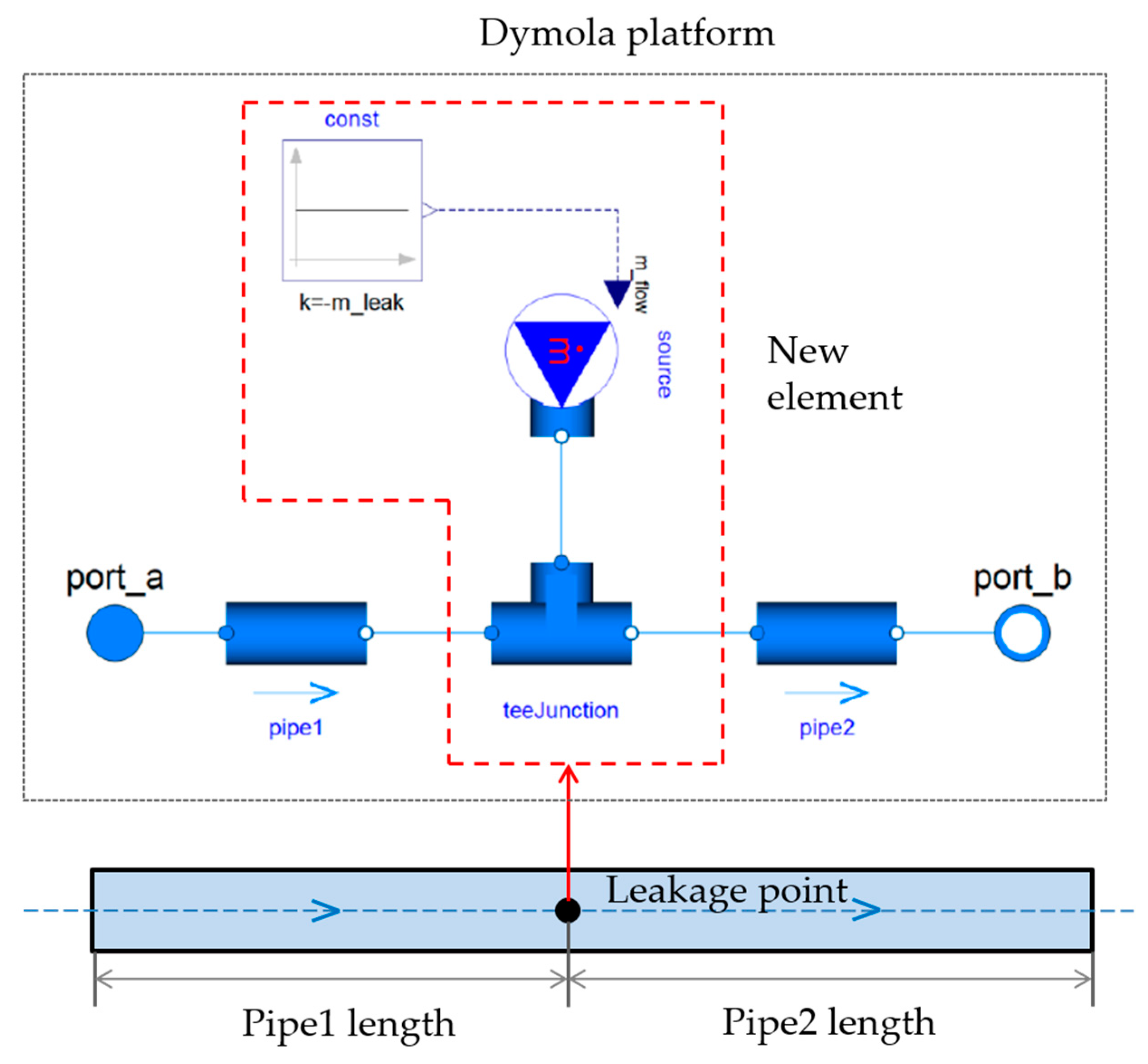
2.2.1. Hydraulic Model of the ACWS Network under Simulated Leakage Conditions
2.2.2. Cuckoo Search Algorithm for the Identification of Network Resistance Characteristics
2.2.3. Adam Optimization Algorithm for the LFD Model
2.2.4. LFD Model Performance Evaluation Indicators
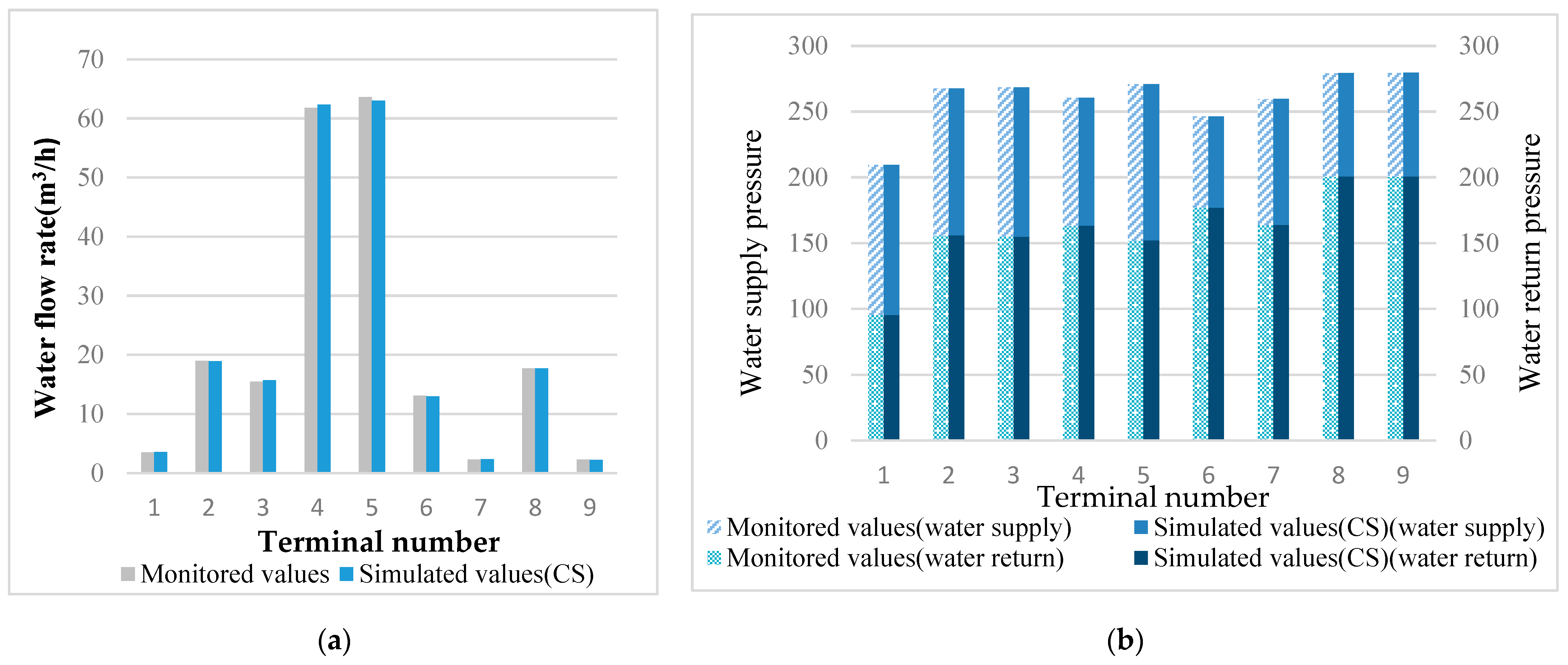
2.3. Case Study
3. Results
3.1. Results of Identification of the Case Pipe Network’s Characteristics
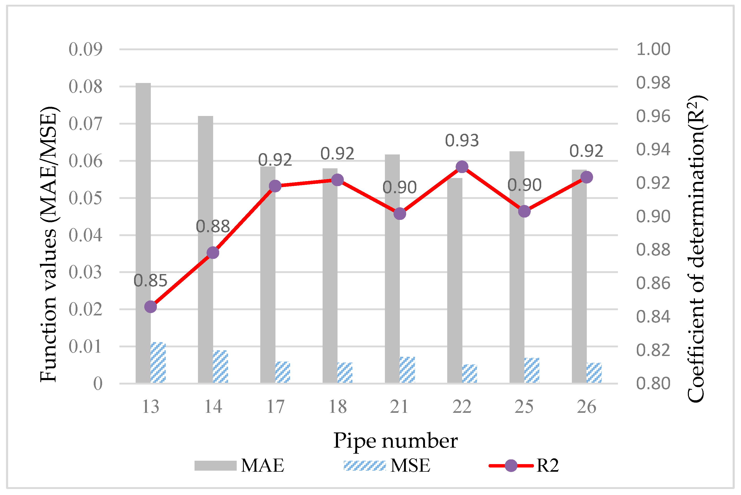
3.2. Results of the First-Stage LFD Model
3.3. Results of the Second-Stage LFD Model
4. Discussions
4.1. Two-Stage LFD Model Discussion
4.2. Limitations
5. Conclusions
Author Contributions
Funding
Institutional Review Board Statement
Informed Consent Statement
Data Availability Statement
Conflicts of Interest
Appendix A

| Number | Leakage Volume (L/s) | Leakage Location | Pressure Difference between the Inlet and Outlet of the Pipe (kPa) | Relative Error (%) | |
|---|---|---|---|---|---|
| Theoretical Value | Simulated Value | ||||
| 1 | 0 | 0 | 19.011 | 18.962 | −0.257 |
| 2 | 0.1 | 0.1 | 18.675 | 18.627 | −0.260 |
| 3 | 0.5 | 0.1 | 17.365 | 17.318 | −0.273 |
| 4 | 1.0 | 0.1 | 15.802 | 15.757 | −0.289 |
| 5 | 0.1 | 0.5 | 18.825 | 18.756 | −0.365 |
| 6 | 0.5 | 0.5 | 18.097 | 18.049 | −0.266 |
| 7 | 1.0 | 0.5 | 17.288 | 17.181 | −0.273 |
| 8 | 0.1 | 0.9 | 18.974 | 18.925 | −0.258 |
| 9 | 0.5 | 0.9 | 18.828 | 18.780 | −0.259 |
| 10 | 1.0 | 0.9 | 18.655 | 18.606 | −0.261 |
References
- Wang, J.; Huang, J.; Fu, Q.; Gao, E.; Chen, J. Metabolism-based ventilation monitoring and control method for COVID-19 risk mitigation in gymnasiums and alike places. Sustain. Cities Soc. 2022, 80, 103719. [Google Scholar] [CrossRef] [PubMed]
- Li, H.; Li, H.; Pei, H.; Li, Z. Leakage detection of HVAC pipeline network based on pressure signal diagnosis. Build. Simul. 2019, 12, 617–628. [Google Scholar] [CrossRef]
- Lu, Y. Practical Heating and Air Conditioning Design Manual. Heat. Vent. Air Cond. 2008, 6, 152. [Google Scholar]
- Mulligan, S.; Hannon, L.; Ryan, P.; Nair, S.; Clifford, E. Development of a data driven FDD approach for building water networks: Water distribution system performance assessment rules. J. Build. Eng. 2021, 34, 101773. [Google Scholar] [CrossRef]
- Puust, R.; Kapelan, Z.; Savic, D.A.; Koppel, T. A review of methods for leakage management in pipe networks. Urban Water J. 2010, 7, 25–45. [Google Scholar] [CrossRef]
- Datta, S.; Sarkar, S. A review on different pipeline fault detection methods. J. Loss Prev. Process Ind. 2016, 41, 97–106. [Google Scholar] [CrossRef]
- Zhou, Z.; Zhang, J.; Huang, X.; Zhang, J.; Guo, X. Trend of soil temperature during pipeline leakage of high-pressure natural gas: Experimental and numerical study. Measurement 2020, 153, 107440. [Google Scholar] [CrossRef]
- Zhou, S.; O’neill, Z.; O’neill, C. A review of leakage detection methods for district heating networks. Appl. Therm. Eng. 2018, 137, 567–574. [Google Scholar] [CrossRef]
- Abdulshaheed, A.; Mustapha, F.; Ghavamian, A. A pressure-based method for monitoring leaks in a pipe distribution system: A Review. Renew. Sustain. Energy Rev. 2017, 69, 902–911. [Google Scholar] [CrossRef]
- Akkaya, A.E.; Talu, M.F. Extended kalman filter based IMU sensor fusion application for leakage position detection in water pipelines. J. Fac. Eng. Archit. Gazi Univ. 2017, 32, 1393–1404. [Google Scholar]
- Abdulla, M.B.; Herzallah, R. Probabilistic multiple model neural network based leak detection system: Experimental study. J. Loss Prev. Process Ind. 2015, 36, 30–38. [Google Scholar] [CrossRef] [Green Version]
- Shen, Y.; Chen, J.; Fu, Q.; Wu, H.; Wang, Y.; Lu, Y. Detection of District Heating Pipe Network Leakage Fault Using UCB Arm Selection Method. Buildings 2021, 11, 275. [Google Scholar] [CrossRef]
- Zadkarami, M.; Shahbazian, M.; Salahshoor, K. Pipeline leakage detection and isolation: An integrated approach of statistical and wavelet feature extraction with multi-layer perceptron neural network (MLPNN). J. Loss Prev. Process Ind. 2016, 43, 479–487. [Google Scholar] [CrossRef]
- Lei, C.; Zhou, P. Application of neural network in heating network leakage fault diagnosis. J. Southeast Univ. (Engl. Ed.) 2010, 26, 173–176. [Google Scholar]
- Duan, P.; Duan, L.; Tian, Q. ANFIS in Leakage Fault Diagnosis of Heating Networks. J. Zhengzhou Univ. (Eng. Sci.) 2014, 35, 56–60. [Google Scholar]
- Xue, P.; Jiang, Y.; Zhou, Z.; Chen, X.; Fang, X.; Liu, J. Machine learning-based leakage fault detection for district heating networks. Energy Build. 2020, 223, 110161. [Google Scholar] [CrossRef]
- Banjara, N.K.; Sasmal, S.; Voggu, S. Machine learning supported acoustic emission technique for leakage detection in pipelines. Int. J. Press. Vessel. Pip. 2020, 188, 104243. [Google Scholar] [CrossRef]
- Duan, H.F. Development of a TFR-Based Method for the Simultaneous Detection of Leakage and Partial Blockage in Water Supply Pipelines. J. Hydraul. Eng. 2020, 146, 04020051. [Google Scholar] [CrossRef]
- Hamza, G.; Hammadi, M.; Barkallah, M.; Choley, J.Y.; Riviere, A.; Louati, J.; Haddar, M. Compact Analytical Models for Vibration Analysis in Modelica/Dymola: Application to the Wind Turbine Drive Train System. J. Chin. Soc. Mech. Eng. 2018, 39, 121–130. [Google Scholar]
- Civicioglu, P.; Besdok, E. A conceptual comparison of the Cuckoo-search, particle swarm optimization, differential evolution and artificial bee colony algorithms. Artif. Intell. Rev. 2013, 39, 315–346. [Google Scholar] [CrossRef]
- Iacca, G.; Dos Santos Junior, V.C.; De Melo, V.V. An improved Jaya optimization algorithm with Levy flight. Expert Syst. Appl. 2021, 165, 113902. [Google Scholar] [CrossRef]
- Yi, D.; Ahn, J.; Ji, S. An Effective Optimization Method for Machine Learning Based on ADAM. Appl. Sci. 2020, 10, 1073. [Google Scholar] [CrossRef] [Green Version]
- Fan, Q.; Guo, Y.; Wu, S.; Liu, X. Two-Level Diagnosis of Heating Pipe Network Leakage Based on Deep Belief Network. IEEE Access 2019, 7, 182983–182992. [Google Scholar] [CrossRef]
- Wen, L.; Li, X.Y.; Gao, L. A New Two-Level Hierarchical Diagnosis Network Based on Convolutional Neural Network. IEEE Trans. Instrum. Meas. 2020, 69, 330–338. [Google Scholar] [CrossRef]
- Fu, Q.; Li, K.; Chen, J.; Wang, J.; Lu, Y.; Wang, Y. Building Energy Consumption Prediction Using a Deep-Forest-Based DQN Method. Buildings 2022, 12, 131. [Google Scholar] [CrossRef]
- Qin, F.W.; Bai, J.; Yuan, W.Q. Research on intelligent fault diagnosis of mechanical equipment based on sparse deep neural networks. J. Vibroeng. 2017, 19, 2439–2455. [Google Scholar] [CrossRef]
- Wang, J.; Hou, J.; Chen, J.; Fu, Q.; Huang, G. Data mining approach for improving the optimal control of HVAC systems: An event-driven strategy. J. Build. Eng. 2021, 39, 102246. [Google Scholar] [CrossRef]
- Ozarisoy, B. Energy effectiveness of passive cooling design strategies to reduce the impact of long-term heatwaves on occupants’ thermal comfort in Europe: Climate change and mitigation. J. Clean. Prod. 2022, 330, 129675. [Google Scholar] [CrossRef]
- Ozarisoy, B.; Altan, H. Regression forecasting of ‘neutral’ adaptive thermal comfort: A field study investigation in the south-eastern Mediterranean climate of Cyprus. Build. Environ. 2021, 202, 108013. [Google Scholar] [CrossRef]
- Sun, J.L.; Wang, R.H.; Duan, H.F. Multiple-fault detection in water pipelines using transient-based time-frequency analysis. J. Hydroinform. 2016, 18, 975–989. [Google Scholar] [CrossRef] [Green Version]


| Performance Evaluation Indicators | Definitions | |
|---|---|---|
| First-stage diagnosis model | ||
| Second-stage diagnosis model | (mean squared error) | |
| MAE (mean absolute error) | ||
| (coefficient of determination) |
| Parameter | Setting |
|---|---|
| Population size of each generation | 50 |
| Discovery probability | 0.25 |
| Maximum number of iterations | 100 |
| Parameter | Setting |
|---|---|
| Number of hidden layer nodes | 31 |
| Activation function of hidden layer | Identity function |
| Regularization parameter | 0.0001 |
| Maximum number of iterations | 3000 |
| Convergence precision | 1 × 10⁻⁴ |
| Pipe Number | Coefficient of Pipe Resistance Characteristic (s2/m5) | Pipe Number | Coefficient of Pipe Resistance Characteristic (s2/m5) |
|---|---|---|---|
| 1 | 53.3 | 16 | 588.0 |
| 2 | 24.0 | 17 | 6188.9 |
| 3 | 267.4 | 18 | 6749.5 |
| 4 | 277.5 | 19 | 32,186.2 |
| 5 | 487,138.3 | 20 | 32,118.5 |
| 6 | 344,413.0 | 21 | 119,729.4 |
| 7 | 2257.2 | 22 | 115,777.9 |
| 8 | 2249.1 | 23 | 426,030.6 |
| 9 | 11,666.6 | 24 | 383,965.0 |
| 10 | 11,909.8 | 25 | 52,034.0 |
| 11 | 12,438.9 | 26 | 43,475.3 |
| 12 | 12,068.8 | 27 | 7121.1 |
| 13 | 4295.8 | 28 | 7064.7 |
| 14 | 4421.0 | 29 | 347,589.0 |
| 15 | 718.9 | 30 | 414,020.7 |
| Pipe Number | Precision (P) | Recall (R) | Pipe Number | Precision (P) | Recall (R) | ||
|---|---|---|---|---|---|---|---|
| 1 | 62.40% | 66.53% | 0.6440 | 16 | 66.07% | 66.65% | 0.6636 |
| 2 | 64.85% | 66.18% | 0.6551 | 17 | 92.39% | 85.90% | 0.8902 |
| 3 | 51.19% | 51.55% | 0.5137 | 18 | 95.58% | 90.14% | 0.9278 |
| 4 | 57.51% | 60.86% | 0.5914 | 19 | 96.08% | 95.91% | 0.9599 |
| 5 | 99.47% | 98.19% | 0.9882 | 20 | 93.68% | 95.21% | 0.9444 |
| 6 | 99.64% | 97.90% | 0.9876 | 21 | 99.06% | 98.54% | 0.9880 |
| 7 | 72.19% | 73.08% | 0.7263 | 22 | 99.52% | 97.13% | 0.9831 |
| 8 | 84.09% | 84.98% | 0.8453 | 23 | 99.11% | 98.24% | 0.9868 |
| 9 | 93.16% | 91.86% | 0.9251 | 24 | 97.60% | 97.49% | 0.9755 |
| 10 | 95.38% | 92.93% | 0.9414 | 25 | 97.85% | 92.82% | 0.9527 |
| 11 | 93.41% | 92.10% | 0.9251 | 26 | 96.50% | 91.98% | 0.9418 |
| 12 | 94.61% | 95.67% | 0.9514 | 27 | 92.54% | 98.01% | 0.9520 |
| 13 | 89.31% | 89.67% | 0.8949 | 28 | 89.66% | 96.37% | 0.9289 |
| 14 | 91.69% | 91.80% | 0.9174 | 29 | 98.44% | 96.48% | 0.9745 |
| 15 | 57.31% | 60.13% | 0.5869 | 30 | 97.47% | 94.62% | 0.9602 |
Publisher’s Note: MDPI stays neutral with regard to jurisdictional claims in published maps and institutional affiliations. |
© 2022 by the authors. Licensee MDPI, Basel, Switzerland. This article is an open access article distributed under the terms and conditions of the Creative Commons Attribution (CC BY) license (https://creativecommons.org/licenses/by/4.0/).
Share and Cite
Liu, R.; Zhang, Y.; Li, Z. Leakage Diagnosis of Air Conditioning Water System Networks Based on an Improved BP Neural Network Algorithm. Buildings 2022, 12, 610. https://doi.org/10.3390/buildings12050610
Liu R, Zhang Y, Li Z. Leakage Diagnosis of Air Conditioning Water System Networks Based on an Improved BP Neural Network Algorithm. Buildings. 2022; 12(5):610. https://doi.org/10.3390/buildings12050610
Chicago/Turabian StyleLiu, Rundong, Yuhang Zhang, and Zhengwei Li. 2022. "Leakage Diagnosis of Air Conditioning Water System Networks Based on an Improved BP Neural Network Algorithm" Buildings 12, no. 5: 610. https://doi.org/10.3390/buildings12050610
APA StyleLiu, R., Zhang, Y., & Li, Z. (2022). Leakage Diagnosis of Air Conditioning Water System Networks Based on an Improved BP Neural Network Algorithm. Buildings, 12(5), 610. https://doi.org/10.3390/buildings12050610