Comparative Evaluation of Different Multi-Agent Reinforcement Learning Mechanisms in Condenser Water System Control

Abstract

Model-free reinforcement learning (RL) techniques are currently drawing attention in the control of heating, ventilation, and air-conditioning (HVAC) systems due to their minor pre-conditions and fast online optimization. The simultaneous optimal control of multiple HVAC appliances is a high-dimensional optimization problem, which single-agent RL schemes can barely handle. Hence, it is necessary to investigate how to address high-dimensional control problems with multiple agents. To realize this, different multi-agent reinforcement learning (MARL) mechanisms are available. This study intends to compare and evaluate three MARL mechanisms: Division, Multiplication, and Interaction. For comparison, quantitative simulations are conducted based on a virtual environment established using measured data of a real condenser water system. The system operation simulation results indicate that (1) Multiplication is not effective for high-dimensional RL-based control problems in HVAC systems due to its low learning speed and high training cost; (2) the performance of Division is close to that of the Interaction mechanism during the initial stage, while Division’s neglect of agent mutual inference limits its performance upper bound; (3) compared to the other two, Interaction is more suitable for multi-equipment HVAC control problems given its performance in both short-term (10% annual energy conservation compared to baseline) and long-term scenarios (over 11% energy conservation).

1. Introduction

As the main place for modern human daily activities [1], buildings account for over 30% of total society energy consumption worldwide [2,3,4]. Moreover, the optimal control of building energy systems, especially heating, ventilation, and air-conditioning (HVAC) systems, can help reduce both building energy consumption and carbon emissions [2,5,6]. As a sub-system of the HVAC system, a condenser water loop accounts for the heat rejection of the central chiller plant. Moreover, the operation quality of this loop can considerably influence the overall efficiency of the whole HVAC system [5,6,7,8,9,10,11]. The control subject of this study is the condenser water loop.

1.1. Value and Application of Reinforcement Learning (RL) Techniques in HVAC System Control

As previously mentioned, the optimal control of HVAC systems is necessary. Before 2013, model-based control (such as the optimal control methods proposed by Kang et al. [10], Huang et al. [8], and other researchers) was the mainstream of the building optimal control field [2]. Apart from this, model-free optimal control based on RL has been drawing increasingly more attention in the building system control domain since 2013 [2]. Generally, there are several reasons for this phenomenon:

(1)

As stated in Ref. [11], model-based control methods’ heavy dependence on accurate system performance models is the main barrier between academic control approaches and practical engineering applications: an accurate model requires integral sensor systems, extensive manual labor, and time to build [8]; moreover, model uncertainty and inaccuracy may harm control performance [12,13].

(2)

Model-free reinforcement learning is a discipline that concerns the fast training of self-learning agents for games and optimal control problems [14]. Its independence from embedded models is suitable to mitigate the “model dependency” issue. The model-free nature of this technique leads to fewer pre-conditions and faster online computation, which enhance its feasibility in building control applications.

Wang and Hong [2] reviewed RL-based building optimal control studies conducted in the last twenty years. In buildings, RL techniques have been used to control various subjects from windows and batteries to hot domestic water systems and HVAC systems. In the HVAC system control field, control variables include the indoor temperature setpoint [15], chilled water temperature setpoint [10,16], and the cooling tower fan frequency [11].

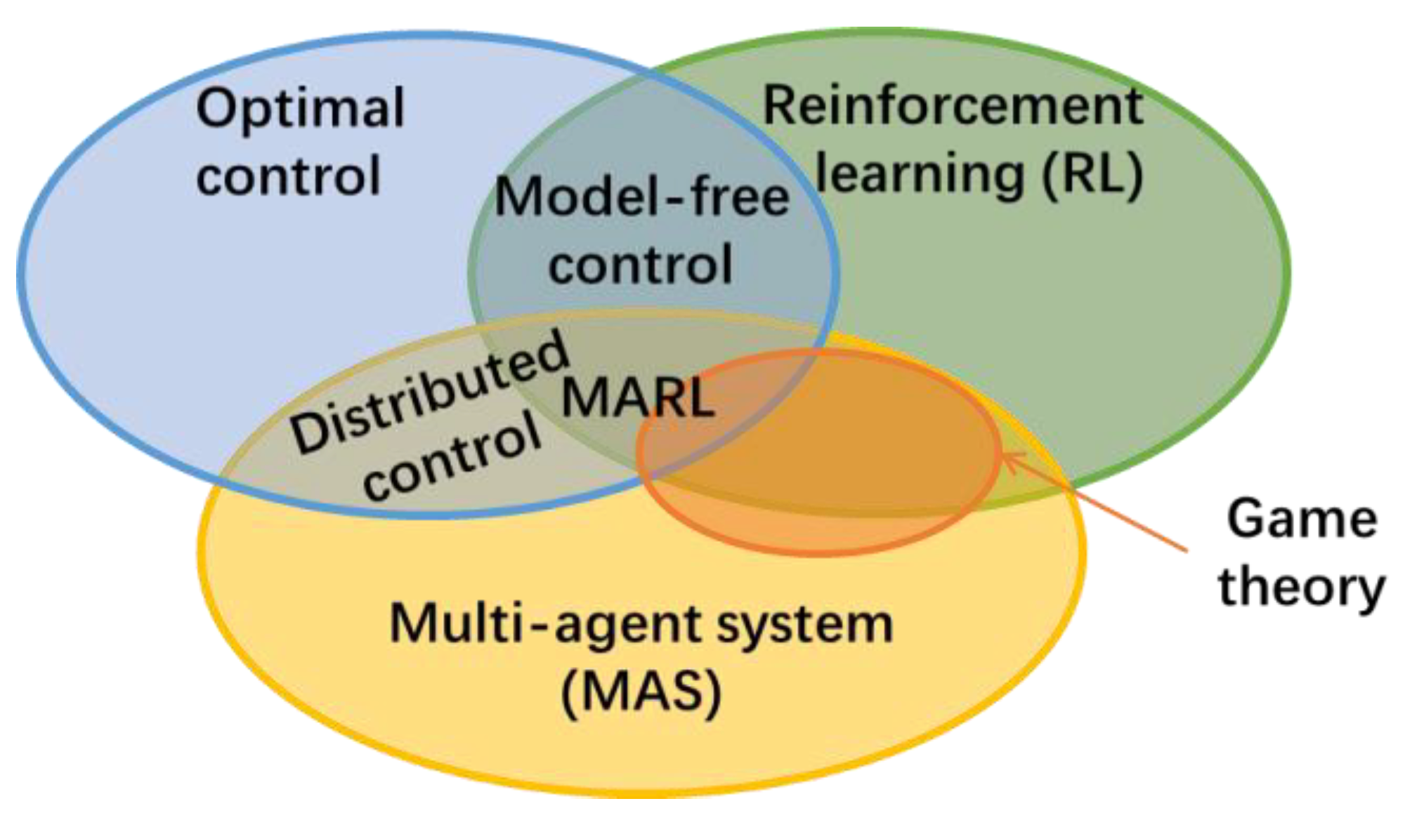
1.2. Multi-Agent Reinforcement Learning (MARL)

The studies reviewed in Ref. [2] mostly applied the single-agent RL scheme to optimize the operation of building energy systems; in the single-agent RL scheme, only one RL agent is set up and used in the control process. When using this technique, the single agent needs to optimize all targeted controllable equipment. When the number of optimized variables grows, the state space and action space of the single agent can grow exponentially, which may lead to unaffordable training costs [17].

To solve the training problem above, one practical method is to decompose the overall control task into several sub-tasks and then assign them to multiple RL agents; these agents then make a multi-agent system (MAS). For instance, Ref. [11] chose to establish two RL agents in order to control the condenser water pump frequency and cooling tower frequency. In doing so, the high-dimensional problem of the single-agent RL scheme could be solved; however, another problem occurred: mutual inference among multiple agents.

As we know, in every time step, an RL agent interacts with the environment: the agent observes the state $s$ of the environment, it takes an action $a$ to control the targeted subject, and then it acquires the reward $r$ from the environment; in the meantime, the environment changes to a new state $s^{\prime }$. In this process, the outputs (the consequent reward $r$ and new state $s^{\prime }$) are determined by the inputs $\left(s,a\right),$ along with the transition probability of the environment $p\left(s^{\prime },r|s,a\right)$ [14,18].

For an MAS, the input of transition probability is composed of the former state and all agents’ actions: $p\left(s^{\prime },r_1,r_2,\dots |s,a_1,a_2,\dots \right)$ [18,19,20]. Hence, the influence of the other agent(s) on the environment needs to be considered, but how [21]? If other agents’ actions are completely observed by Agent 1, then there will be a huge observable variable space for it, and the learning cost may be unacceptable similarly to the single-agent RL scheme. If not, then it may be hard for Agent 1 to learn and evolve due to invisible inference from other agents.

To solve the MAS problem above, multi-agent reinforcement learning (MARL) has been proposed [22]. The relationship among four research domains is illustrated in Figure 1. “Distributed control” is designed to solve the system optimization problem with multiple optimizers (could be model based, RL based, etc.) instead of one centralized optimizer [23]. Moreover, MARL is the intersection of the optimal control problem, the MAS environment, game theory, and RL techniques.

MARL techniques are intended to make each agent learn fast and well in an MAS where mutual inference is inevitable. Moreover, scenarios can be divided into three types (fully cooperative, non-fully cooperative, and fully competitive) depending on whether the agents’ objectives are consistent [18]. Only the fully cooperative problem is discussed in this article, because generally, all equipment in an HVAC system works collaboratively to maintain an acceptable built environment and energy efficiency.

Classic MARL algorithms include Nash Q-learning, Friend-or-Foe, Win or Learn Fast–Policy Hill Climbing (WoLF-PHC), and the multi-agent deep deterministic policy gradient (MADDPG) [18,19,24,25]. Generally, MARL mechanisms can be categorized into Division, Multiplication, and Interaction [26].

Division mechanism: this means that each agent in the MAS learns and works by itself on its own task without considering the potential inference caused by other agents. Independent Q-learning (IQL) is a typical Division algorithm [26,27,28,29]. For instance, Yang et al. [30] set up three RL agents to control three loops in a low-exergy building model. Although the three controlled loops were physically related, no measure was specifically taken for the mutual inference among the agents. However, since their targeted problem was a fully-cooperative game, choosing the Division mechanism still achieved acceptable performance [18,31].

Multiplication mechanism: this is somewhat of a brute. In this scheme, multiple agents are simply piled up in one MAS. Each agent needs to act like a generalist who is capable of carrying out all activities [26]. As far as we are concerned, the single-agent scheme (where one central controller undertakes everything) is simply a special case of the Multiplication mechanism. In this study, we realize Multiplication by merging all RL agents in the MAS into one single agent. In doing so, the action spaces of the former agents are multiplied to one, and the inference problem in the MAS is eradicated [32]. However, the action space of this single agent is enormous due to the dimension increase.

Interaction mechanism: this is specifically designed for the MARL problem; in this scheme, the mutual inference problem is positively handled, and each agent in the MAS actively adapts to this non-Markovian dynamic environment knowing that there are others out there [26]. Moreover, the MAS reaches its optimum (in a fully cooperative MARL problem) or equilibrium (in a non-fully cooperative MARL problem) faster [18,24,25]. For instance, Tao et al. [17] proposed a cooperative learning strategy based on WoLF-PHC. Their proposed strategy was tested on the Keepaway game of RoboCup, and their results suggest that a cooperative learning strategy can outperform the scheme of tag match learning (where each single agent takes turns to learn from the environment).

In this article, we quantitatively compare these three mechanisms in the optimal control problem of building condenser water loops. Moreover, the methodologies are elaborated on in Section 3.

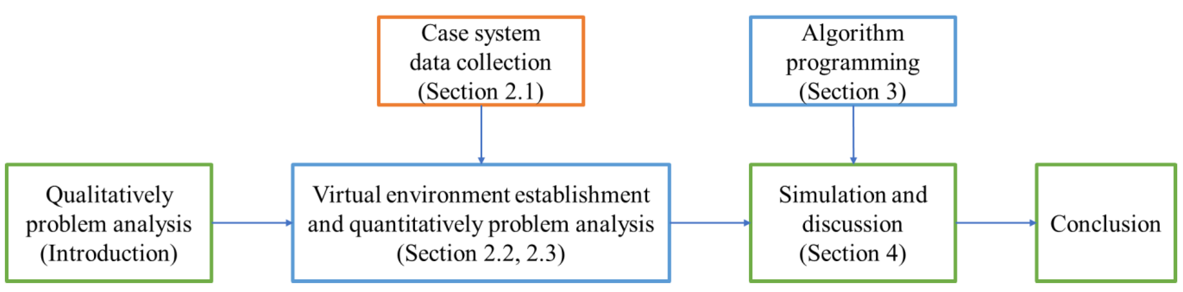
1.3. Motivation and Overall Framework of this Research

To sum up, the optimal control of HVAC systems is important for building energy conservation and decarbonization; model-free RL control has been drawing attention in the HVAC optimal control domain due to its independence from models; when multiple HVAC appliances need to be controlled with RL-based methods, the mutual inference problem occurs; and this study investigates the feasibility of different MARL mechanisms in the RL-based HVAC optimal control problem.

The overall framework/workflow of this research is illustrated in Figure 2. This article first qualitatively discusses the targeted problem in the Introduction. Then, Section 2 demonstrates the establishment and verification of a virtual environment, which is used in the simulation case study. Based on this environment, Section 2 quantitatively analyzes the mutual inference problem in an MAS. Section 3 introduces the methodology of the three MARL mechanisms, and Section 4 presents and discusses the control performances of comparative controllers in the virtual environment.

2. Virtual Environment Establishment

In this study, the control performances of three different MARL mechanisms are evaluated using simulations. Moreover, the simulations are based on a virtual environment (i.e., system performance model). To enhance the actual meaning of the simulations herein, a real HVAC system with measured operational data is selected as the case system. Due to thorough commissioning and maintenance before data collection, its operational data are of high quality; hence, the data are used for data-driven system modeling in this study. This section demonstrates the establishment of the system model, based on which a quantitative analysis is conducted on the mutual inference problem in an MAS.

2.1. Case System

The layout of the case condenser water system is shown in Figure 3, and the characteristics are listed in

Table 1. Condenser water system characteristics.

Equipment	Number	Characteristics
Screw chiller	2	Cooling capacity = 1060 kW, power = 159.7 kW
Condenser water pump	2 + 1 (one auxiliary)	Power = 14.7 kW, flowrate = 240 m3/h Head: 20 m, variable speed
Cooling tower	2	Power = 7.5 kW, flowrate = 260 m3/h, variable speed

. Its 2019 cooling season field data are adopted to establish the virtual environment for the simulations. It should be noted that, generally, the Chinese cooling season is defined as June to September, which is when mechanical cooling is necessary in buildings. However, the actual cooling season of each city is related to the local climate. In this study, the operational data of the real case system from 1 June to 18 September 2019 are collected, during which the case system was almost continuously supplying cooling. Hence, this period is regarded as one cooling season in the simulations herein.

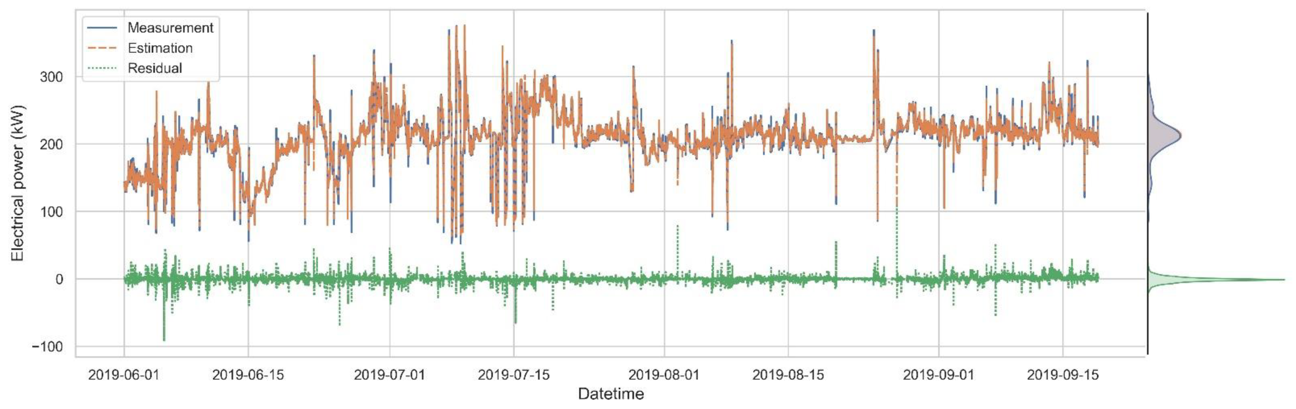
2.2. Field-Data-Based System Modeling

The virtual environment is established based on a black-box regressor random forest (with default hyper-parameters by sci-kit learn Python package [33]) and the 2019 cooling season field data of the case system (from 1 June to 18 September, with data sampling intervals of 10 min). Equation (1) is proposed to model the real-time electrical power of the whole condenser water loop. The involved variables are introduced in

Table 2. Nomenclature of involved variables.

Variable	Description	Unit
$P_{system}$	Real-time overall system electrical power	kW
$C{L}_s$	System cooling load	kW
$T_{wet}$	Ambient wet-bulb temperature	°C
$f_{pump}$	Common frequency of running condenser water pump(s)	Hz
$n_{pump}$	Current working number of condenser water pumps
$f_{tower}$	Working frequency of running cooling tower(s)	Hz
$n_{tower}$	Current working number of cooling towers
$T_{chws}$	Temperature of supplied chilled water	°C
$statu{s}_{chiller}$	Current working status of chillers: 1—only Chiller 1 is running, 2—only Chiller 2 is running, 3—both chillers are running, 0—no chiller is running

.

$$P_{system}=Random forest\left(C{L}_s,T_{wet},f_{pump}, n_{pump},f_{tower},n_{tower}, statu{s}_{chiller},T_{chws}\right)$$

(1)

The undetermined coefficients in Equation (1) are determined using regression with measured field data. The running dataset (when the system is running) is selected, and then it is randomly divided into a training set (80%) and a testing set (20%) to train and verify the black-box model, respectively. The coefficient of variation of the root mean square error (CV-RMSE) and the coefficient of determination (R²) are used to evaluate the reliability of the trained model. In Equations (2) and (3), n is the length of the dataset, $y_i$ is the i^th measured value of the system power, and $\widehat{y_i}$ is the corresponding estimated value. $\overline{y}$ is the mean value of all $y_i$s. The detailed calculation process of model error indicators can be found in ASHRAE Guideline 14 [34,35].

$$CV-RMSE=\frac{\sqrt{n{{\displaystyle \sum }}_{i=1}^n{\left(y_i-\widehat{y_i}\right)}^2}}{{{\displaystyle \sum }}_{i=1}^n{y}_i}$$

(2)

$$R^2=1-\frac{{{\displaystyle \sum }}_1^n{\left(y_i-\widehat{y_i}\right)}^2}{{{\displaystyle \sum }}_1^n{\left(y_i-\overline{y}\right)}^2}$$

(3)

The time-series data of the estimated power, measured power, and absolute residuals are illustrated in Figure 4. The right side of the figure shows the distribution of the three variables; the estimation errors mainly lie within a narrow range around 0, which means that the estimation error is mild. The calculated indicator values are listed in

Table 3. Error index values of the trained model.

	Training Set	Testing Set
CV(RMSE)	1.48%	3.76%
R2	0.99	0.95

. According to Page 97 of ASHRAE Guideline 14 [34], CV-RMSE below 30% is acceptable for hourly building energy modeling. Hence, the established model is reliable for the following simulations in 10 min time-step intervals.

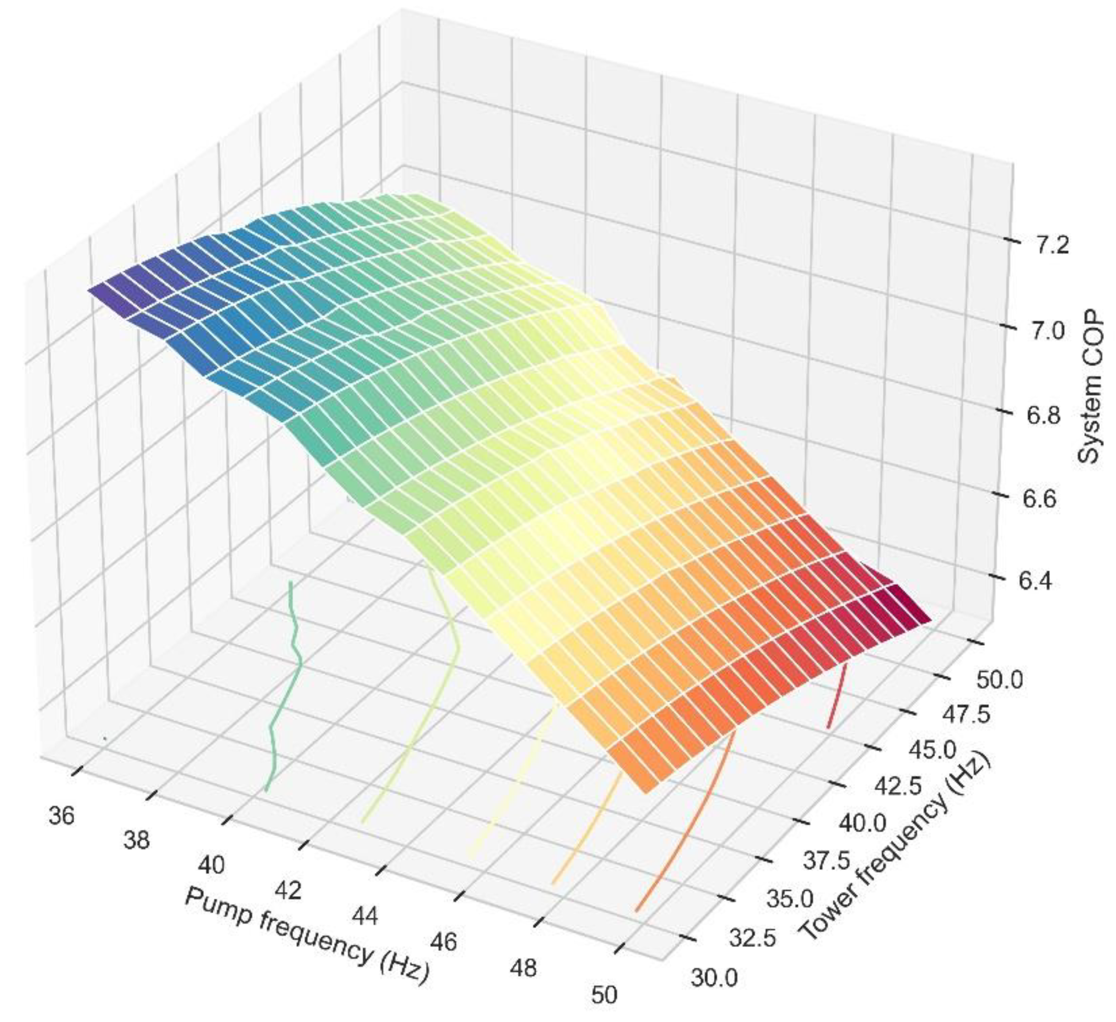
2.3. Mutual Inference between Cooling Tower Action and Condenser Water Pump Action

The operation objective of a condenser water loop is to maximize its overall energy efficiency. Herein, we take the comprehensive coefficient of performance (COP, calculated using Equation (4)) of these appliances as our optimization objective and quantitatively analyze the MAS mutual inference problem between cooling towers and condenser water pumps.

Figure 5 shows the system modeling result under a typical working condition ($C{L}_S=1400 \mathrm{kW},T_{wet}=25.8 ℃,n_{pump}=n_{tower}=2,statu{s}_{chiller}=3,T_{chws}=10 ℃$), with various combinations of tower pump frequencies.

Figure 5 suggests that both pieces of equipment can sufficiently influence the system’s COP. If the system’s COP is chosen as the common reward by the two RL agents (tower agent and pump agent), each agent’s learning process will be influenced by the other one’s movement, as mentioned in Section 1.2. This fact could lead to an uncertain, unstable RL process. Thus, if the condenser water loop is to be controlled by multiple RL agents, the mutual inference problem needs to be considered.

3. Methodology of MARL-Based Controllers

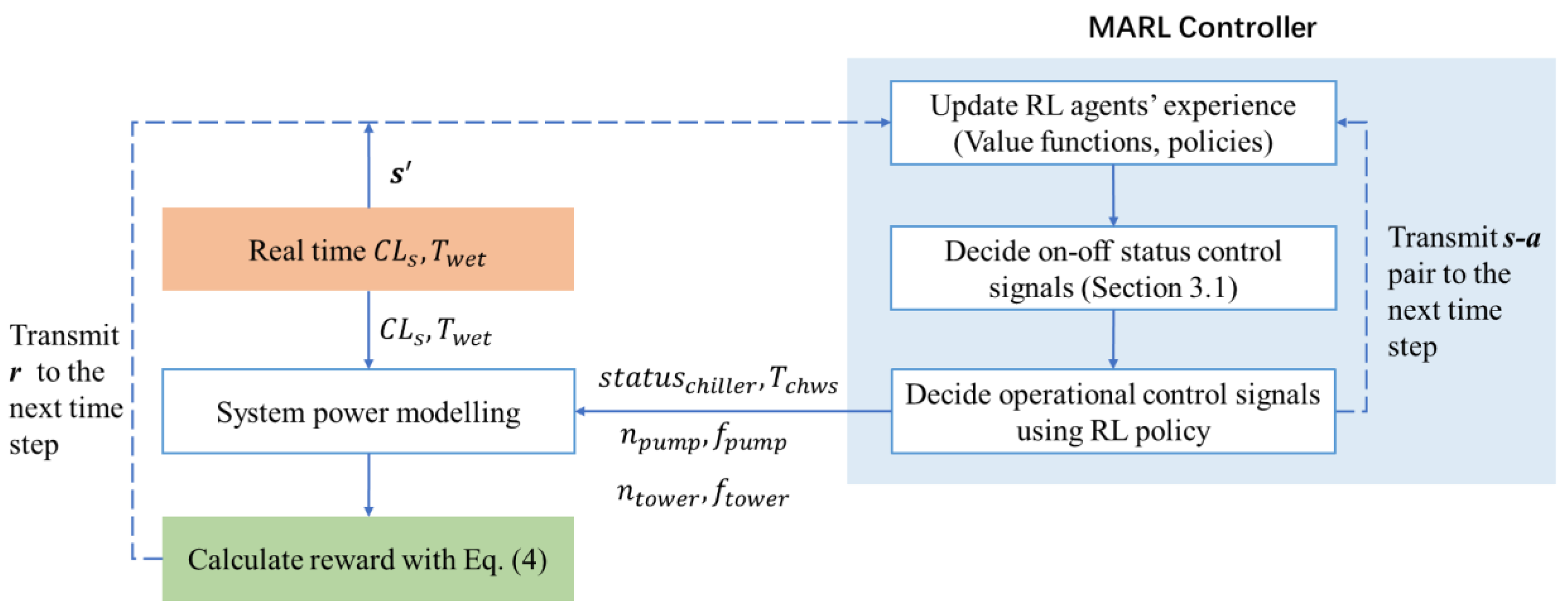
3.1. Overview

As justified in Section 2.3, the inference problem between agents should be carefully handled when multiple RL agents function simultaneously in an MAS. Typical MARL solutions can be categorized into three types: Division, Multiplication, and Interaction [26]. The control performances of these three different MARL mechanisms are compared and evaluated in this study.

In this study, Policy Hill Climbing (PHC) and Win or Learn Fast–Policy Hill Climbing (WoLF-PHC) are selected as specific algorithms for comparison because their complexity, basic thinking, and pre-conditions are similar [20]. In doing so, the performance gap between the MARL mechanisms rather than the specific algorithms can be better revealed. Figure 6 shows a common workflow of the MARL controller interacting with the virtual environment in this study. Every simulation time step occurs as follows:

(1)

Input real-time $C{L}_S$ and $T_{wet}$ (two uncontrollable environmental variables [5]) to the virtual environment (i.e., system model) and the controller.

(2)

Based on the inputs, the controller decides the proper control signals, including on–off control signals and operational signals (i.e., setpoints of $f_{pump}, n_{pump},f_{tower},n_{tower}, statu{s}_{chiller}, \mathrm{and} T_{chws}$).

(3)

Model the electrical power of the system. Calculate the system’s COP (the common reward of RL agents).

(4)

Turn to the next simulation time step.

(5)

RL agents update the experience with the last reward $r$, last state–action ($s-a$) pair, and current state $s^{\prime }$.

Note that, in Figure 6, the solid line indicates that data transmission occurs in the same time step, while the dashed line indicates that data transmission occurs between two adjacent time steps (i.e., the reward calculated in the current time step is not used until the next time step for the agents’ learning).

In this study, the RL agents only decide $f_{pump} \mathrm{and} f_{tower}$, whereas the on–off statuses of all appliances and $T_{chws}$ are controlled according to the following rules:

(1)

To protect chillers from a low partial load ratio (PLR) operation risk, the whole system only operates when $C{L}_s$ is larger than 20% of a single chiller’s cooling capacity [36,37,38].

(2)

In order to fully utilize the heat exchange area of cooling towers, two cooling towers operate simultaneously when the system is on.

(3)

Two chillers operate simultaneously when $C{L}_s$ is larger than a single chiller’s maximum cooling capacity; otherwise, only Chiller 1 operates to cover the cooling demand.

(4)

The number of running condenser water pumps is in accordance with the number of working chillers.

(5)

$T_{chws}$ is set to 11 °C constantly, which is close to the chillers’ nominal value.

The control logic above is used by all controllers in the case study section.

3.2. Division and Multiplication MARL Controllers: Policy Hill Climbing

This section presents the details of Multiplication and Division.

Firstly, for Division, Policy Hill Climbing (PHC) is adopted as the specific algorithm. In PHC, both the value function and policy function are updated in every learning step. The value function is updated based on the real-time reward, which, in turns, directs the updating process of the policy function [39]. Hence, the PHC algorithm is a somewhat simplified version of the actor–critic algorithm but without neural networks and gradient calculation. The two RL agents (the cooling tower agent and condenser water pump agent) are formulated as follows:

State: Real-time $T_{wet}$ and $C{L}_s$ are discretized and combined to the state value such as ($C{L}_S=1060 \mathrm{kW}, and T_{wet}=26 ℃$). The discretization interval of $T_{wet}$ is 1 °C, and the discretization interval of $C{L}_s$ is 10% of a single chiller’s cooling capacity, as shown in Table 1. The two agents share the same state value.

Action: The operating frequencies of the cooling tower fan(s) and the condenser water pump(s) are the action variables of the two agents. The action space of the tower agent is 30–50 Hz (1 Hz interval), and the action space of the pump agent is 35–50 Hz with 1 Hz intervals. Note that on–off statuses and $T_{chws}$ are controlled according to the rules addressed in Section 3.1.

Reward: the common reward (optimization objective) of both agents is the real-time system’s COP, which is calculated using Equation (4):

$$System COP=C{L}_s÷P_{system}$$

(4)

where $C{L}_s$ is the system cooling load (kW), and $P_{system}$ refers to the modeled total electrical power (kW) of the chillers, condenser water pumps, and cooling towers.

Initialization: When applying PHC, the value function $Q_i\left(s,a_i\right)$ and target policy ${\pi }_i\left(s,a_i\right)$ need to be set up for every agent. The values of the value function should be initialized to 0, and the values of ${\pi }_i\left(s,a_i\right)$ should be initialized to $\frac{1}{\left|A_i\right|}$, where $\left|A_i\right|$ is the total action number in the i^th agent’s action space (21 for the tower agent and 16 for the pump agent).

After the off-line agent formulation, the online real-time control process (right side of Figure 6) is realized as follows:

In every simulation time step, each agent updates its own value function and target policy with Equations (5)–(8). The footnote i refers to the agent code (the tower agent is 1, and the pump agent is 2). In Equation (5), $Q_i\left(s,a_i\right)$ is the specific Q-value of the i^th agent corresponding to the last state $s$ and its last action $a_i$. $\alpha$ is the agents’ learning rate, which is set to 0.7 referring to the engineering application in Ref. [16]; $r$ is the reward value from the last time step; $\gamma$ is the weight of the expected future reward, which is set to 0.01 referring to Ref. [16]; and $\underset{a_i{}^{\prime }}{\max }{Q}_i\left(s^{\prime },a_i{}^{\prime }\right)$ is the maximum Q-value of the i^th agent under current state $s^{\prime }$.

$$Q_i\left(s,a_i\right)\leftarrow Q_i\left(s,a_i\right)+\alpha \left[r+\gamma \underset{a_i{}^{\prime }}{\max }{Q}_i\left(s^{\prime },a_i{}^{\prime }\right)-Q_i\left(s,a_i\right)\right]$$

(5)

$${\pi }_i\left(s,a_{i,j}\right)\leftarrow {\pi }_i\left(s,a_{i,j}\right)+{\mathsf{\Delta }}_{s,a_{i,j}}\hspace{1em}\hspace{1em}\mathrm{for} \forall a_{i,j}\in A_i$$

(6)

where

$${\mathsf{\Delta }}_{s,a_{i,j}}=\left\{\begin{array}{c}-{\delta }_{s,a_{i,j}} if a_{i,j}\ne arg\underset{a_i{}^{\prime }}{\max }{Q}_i\left(s,a_i{}^{\prime }\right)\\ {\displaystyle {\displaystyle \sum }_{a_{i,c}\ne a_{i,j}}}{\delta }_{s,a_{i,c}} \mathrm{else}\end{array}\right.$$

(7)

where

$${\delta }_{s,a_{i,j}}=\min \left({\pi }_i\left(s,a_{i,j}\right),\frac{\delta }{\left|A_i\right|-1}\right)$$

(8)

Moreover, Equations (6)–(8) are used for policy updating, the thinking of which is to transfer the “probability to be chosen” from non-optimal actions to the optimal action. The parameter $\delta$ determines the transfer amount in every optimization step. According to Ref. [20], this varies with the case game, and it is set to 0.03 herein.

For the Multiplication RL controller, its offline and online processes are similar to those of Division. The difference is that the Multiplication RL controller only builds one RL agent to control both the cooling towers and condenser water pumps. Hence, its action space is composed of $16\times 21$ jointed actions (pump 35 Hz, tower 30 Hz), (pump 36 Hz, tower 30 Hz), …, (pump 50 Hz, tower 30 Hz), …, (pump 50 Hz, tower 50 Hz). Moreover, this single agent works alone using Equations (5)–(8), with the same state variable, reward variable, and hyperparameters ($\alpha ,\gamma ,\delta$) as those of Division.

3.3. Interaction MARL Controller: WoLF-PHC

Win or Learn Fast–Policy Hill Climbing (WoLF-PHC) is a classic MARL algorithm suitable for fully cooperative and non-fully cooperative problems [17,20,40]. This algorithm is derived from the PHC algorithm, and it is composed of three core functions: the value function $Q_i\left(s,a_i\right)$, the target policy ${\pi }_i\left(s,a_i\right)$, and the historical average policy $\overline{{\pi }_i}\left(s,a_i\right)$.

The core thinking of this algorithm is to determine whether one agent is performing better than before in the learning process by comparing the mathematical expectations of the value function under the target policy and historical average policy (Equation (11)). If the current policy is proven to be better than the historical average, then we can claim that this agent is winning/adapting in this MAS, and its learning pace is mild; otherwise, this agent is not adapting well in this MAS (suppressed by other agents), and this agent then needs to change/update its policy faster to manage. In WoLF-PHC, although the agents do not interact with each other explicitly, each agent is aware of the other agents’ existence and deliberately adapts itself to the dynamic MAS.

When realizing the Interaction mechanism (WoLF-PHC), the offline formulation of the agents is similar to that in the Division mechanism: the two agents (the tower agent and pump agent) are set up with common state variables (jointed discrete $T_{wet}$ and $C{L}_s$) and separated action spaces (30–50 Hz for the tower agent and 35–50 Hz for the pump agent) as described in Section 3.2. The main difference between Interaction and Division in this study is the usage of the historical average policy $\overline{{\pi }_i}\left(s,a_i\right)$ and the dynamic $\delta$. The detailed workflow of WoLF-PHC is presented in

Table 4. Workflow of WoLF-PHC algorithm.

Off-line initialization: For the tower agent and pump agent (footnote i refers to the ith agent), formulate their action spaces and common state spaces in the same way as Division. For each agent, initialize all $Q_i\left(s,a_i\right)$ values to 0, initialize all ${\pi }_i\left(s,a_i\right)$ values to $\frac{1}{\left|A_i\right|}$, and initialize all $\overline{{\pi }_i}\left(s,a_i\right)$ values to $\frac{1}{\left|A_i\right|}$. The number of each state’s occurrence is recorded by $C\left(s\right)$, and it is initialized to 0.

Online decision-making procedure in every time step: Receive reward $r$$\mathrm{and} (s,a_1,a_2$$) \mathrm{of} \mathrm{the} \mathrm{last} \mathrm{time} \mathrm{step}. a_1 \mathrm{and} a_2$ are the last actions of the tower agent and pump agent, respectively. Receive real-time $C{L}_s \mathrm{and} T_{wet}$$$ Then, both agents execute the following procedure parallel:

C. Update the current value function $\left(\mathrm{Q}\text{-}\mathrm{table}\right) \mathrm{with} \mathrm{Equation} \left(5\right) (\alpha =0.7, \gamma =0.01$). D. For $\forall a_{i,j}\in A_i$$, \mathrm{update} \mathrm{its} \mathrm{corresponding} \mathrm{historical} \mathrm{average} \mathrm{policy} \overline{{\pi }_i}\left(s,a_{i,j}\right)$ with Equations (9) and (10)

E. Use the latest Q-table to update the target policy ${\pi }_i\left(s,a_{i,j}\right)$$$$\mathrm{with} \mathrm{Equation} \left(11\right) ({\delta }_{win}=0.01, {\delta }_{lose}=0.05$). F. Decide the next action for current state $s^{\prime }$$\mathrm{with} \mathrm{updated} {\pi }_i\left(s,a_i\right)$

.

$$C\left(s\right)=C\left(s\right)+1$$

(9)

$$\overline{{\pi }_i}\left(s,a_{i,j}\right)\leftarrow \overline{{\pi }_i}\left(s,a_{i,j}\right)+\frac{1}{C\left(s\right)}\left[{\pi }_i\left(s,a_{i,j}\right)-\overline{{\pi }_i}\left(s,a_{i,j}\right)\right]$$

(10)

$$\delta =\left\{\begin{array}{c}{\delta }_{win} \mathrm{if}{\displaystyle {\displaystyle \sum }_{a_{i,j}\in A_i}}{\pi }_i\left(s,a_{i,j}\right)Q_i\left(s,a_{i,j}\right)>{\displaystyle {\displaystyle \sum }_{a_{i,j}\in A_i}}\overline{{\pi }_i}\left(s,a_{i,j}\right)Q_i\left(s,a_{i,j}\right)\\ {\delta }_{lose} \mathrm{else}\end{array}\right.$$

(11)

For WoLF-PHC, the key pre-defined parameters include $\alpha ,\gamma ,{\delta }_{win},\mathrm{and} {\delta }_{lose}$. In this study, $\alpha =0.7,\mathrm{and} \gamma =0.01$, which are the same as Division’s parameters. ${\delta }_{win} \mathrm{and} {\delta }_{lose}$ are the special parameters of WoLF-PHC, and these two parameters determine how fast the agent changes its target policy. According to Refs. [20,39], ${\delta }_{lose}:{\delta }_{win}=4$ is recommended to reach fast convergence. In this study, ${\delta }_{win}=0.01, {\delta }_{lose}=0.05$, which means that, when an agent is adapting well in the MAS (winning), the probability of every non-optimal action to be chosen decreases $\frac{0.01}{\left|{\mathrm{A}}_{\mathrm{i}}\right|-1}$ in every simulation time step (these decreases are transferred to the optimal action); however, when the agent is losing, the probability of every non-optimal action to be chosen decreases $\frac{0.05}{\left|{\mathrm{A}}_{\mathrm{i}}\right|-1}$ in every simulation time step (learn fast). The abovementioned reflects the idea of “Win or Learn Fast”.

4. Simulation Case Study and Discussion

The operation of the case system from 1 June to 18 September is simulated in this section, and it is based on the established system’s black-box model as the virtual environment and the measured data of $T_{wet} \mathrm{and} C{L}_s$ as real-time inputs. Five simulation cases corresponding to five different controllers are conducted to evaluate the energy-saving performance of the three different MARL mechanisms. The simulation process is illustrated in Figure 6, and the case characteristics are listed in

Table 5. Simulation cases.

Case	Controller Algorithm	Tower Agent Action	Pump Agent Action	Parameters	State	Reward
#1	Baseline	50 Hz	50 Hz	/	/	/
#2	PHC (Division)	30–50 Hz	35–50 Hz	α = 0.7 γ = 0.01 δ = 0.03	Twet CLs	System COP
#3	PHC (Multiplication)	Jointed actions such as (pump 50 Hz, tower 30 Hz)
#4	WoLF-PHC (Interaction)	30–50 Hz	35–50 Hz	$\alpha =0.7$ $\gamma =0.01$ ${\delta }_{win}=0.01$ ${\delta }_{lose}=0.05$
#5	PID feedback control	Approach at 2.5 °C	Condenser water ΔT at 3.3 °C	/	/	/

. Note that, since the RL learning process is stochastic, Cases 2–4 are simulated three times to obtain the average results for analysis.

In addition to the three described MARL controllers, there are two typical controllers, namely, the baseline constant speed controller and the proportional–integral–derivative (PID) feedback controller. The constant speed controller keeps the online cooling towers and condenser water pumps running at 50 Hz, the performances of which are taken as the baseline in this study. The logic of the PID feedback controller here is the same as the control logic used in the real case system: (1) adjust the cooling tower frequency to maintain the approach (tower outlet water temperature minus $T_{wet}$) at 2.5 °C, and (2) adjust the condenser water pump frequency to maintain the temperature difference between the supplied condenser water and returned condenser water at 3.3 °C.

Since the system model set up in this study does not model the condenser water temperature, it is not practical to embed PID logic into the system model in Case #5. Instead, the on-site control signal record of the real case system is directly reused to control the virtual environment in Case #5, because the recorded control signals are determined by the real PID controller. Furthermore, it did maintain the monitored temperature variables at their set points for the real system.

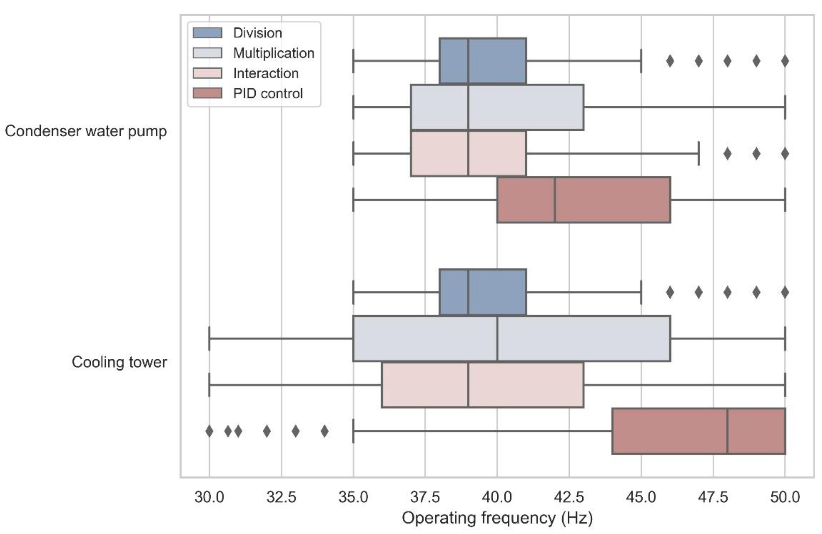
4.1. Short-Term Performance

Table 6. Simulated system energy consumption of each case.

Cases	Total System Energy Consumption over One Cooling Season (kWh)	Energy-Saving Ratio Compared to Baseline (%)
#1 Baseline	543,979	0.00
#2 Division	489,450	10.02
#3 Multiplication	496,869	8.66
#4 Interaction	488,621	10.18
#5 PID feedback	529,933	5.96

lists the simulated system energy consumptions under the five controllers in the first simulated cooling season, and Figure 7 illustrates the equipment frequency distributions under the different controllers. In the first cooling season, all MARL controllers learn to control from ground zero (all agents are initialized during the first simulation step). Moreover, simulated results in this scenario reflect the learning speed of each mechanism, which is an important evaluation indicator of RL algorithms [14,41].

Table 6 suggests that the energy-saving performances of all MARL controllers are better than that of the original PID feedback controller. This result is in accordance with the equipment frequency distribution: the control actions chosen by the original PID controller are more conservative than those of the MARL controllers. This is because the on-site engineers need to seriously consider system safety when configuring the PID control logic, which can result in higher equipment frequency and more energy waste. Different from the original PID logic, MARL controllers are designed to focus on the optimization task, which is system energy efficiency; therefore, they perform better than the original PID controller.

Comparing the performance of the three MARL controllers, it could be seen that Multiplication performs worse than the other two. Moreover, the frequency data under Multiplication are more diffused than those of the others. This is as anticipated in Section 1.2: the Multiplication mechanism typically means a high-dimension action space, which can lead to high exploration costs, long training periods, and poor performance at the initial stage.

The initial performance gap between Division and Interaction is slight. It is inferred that the small performance gap is due to the following reasons: (1) Both Division and Interaction address the case problem with two agents (the action and solution spaces are limited); hence, the learning speed of these two mechanisms are both fast and close to each other. (2) At the initial stage of the RL agents’ learning processes, the performance potential of the RL agents is still far from being fully utilized; thus, Interaction’s advantage of having a higher upper limit cannot be revealed in this short-term scenario. (3) The design of this case study is intended to better investigate the difference among the different MARL mechanisms rather than different RL algorithms; hence, the theoretical gap among the three MARL controllers is not that evident in the first place.

Therefore, the mild performance difference between Division and Interaction in the first cooling season suggests that a short-term experiment may not be sufficient to compare these two MARL mechanisms in the HVAC control field if they are both based on a similar theoretical basis (i.e., Policy Hill Climbing herein). To better reveal the advantage and disadvantage of each MARL mechanism, long-term simulations are conducted in the next section.

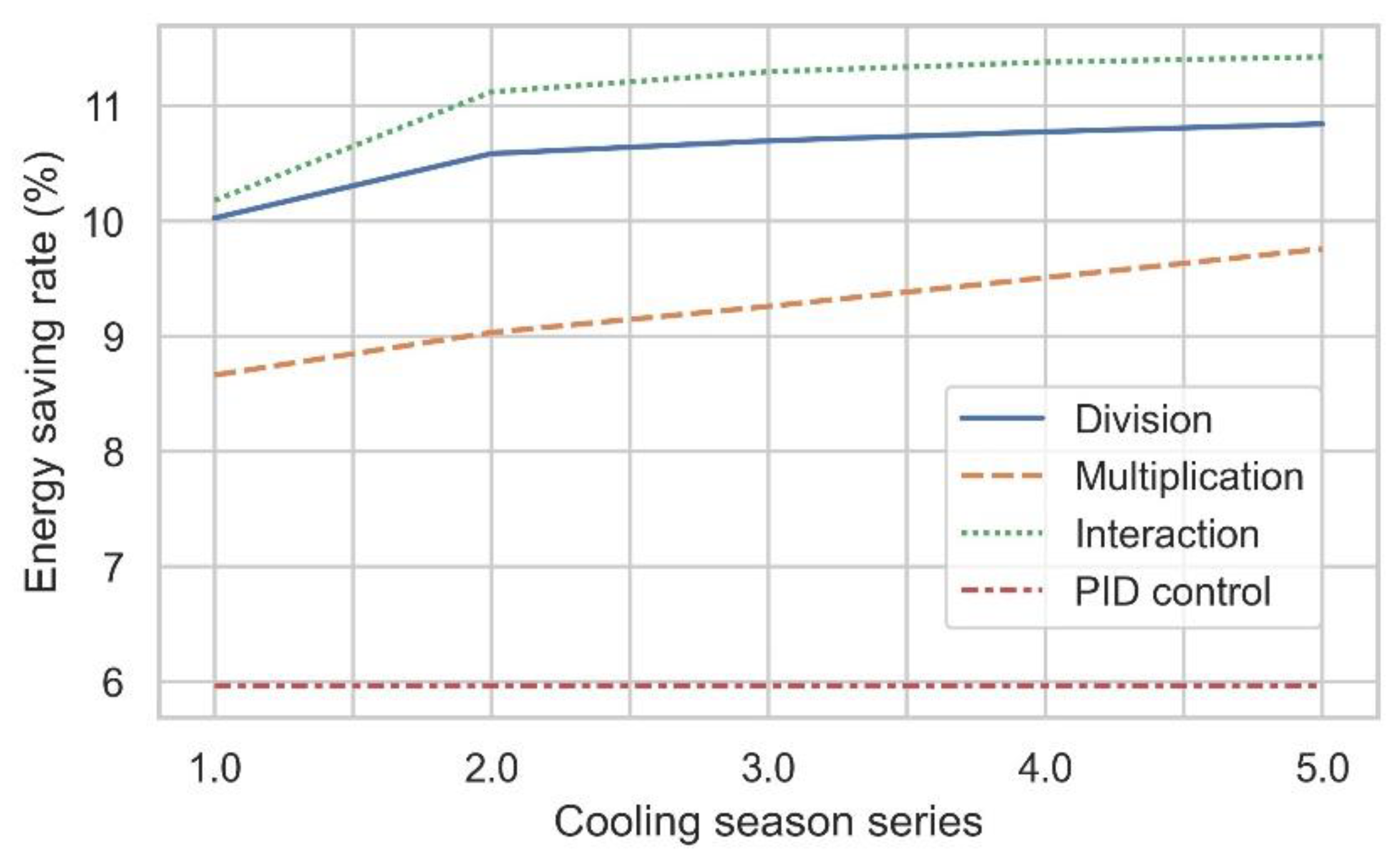
4.2. Long-Term Performance

The post-convergence performance (upper limit) is another critical indicator of RL algorithms [41]. To better analyze the long-term performances of each MARL controller, five-episode continuous simulations are conducted under the three MARL controllers. This is realized by continuously simulating the system’s operation in the same five cooling seasons, without resetting the RL agents midway. In doing so, the long-term evolution of a MARL controller can be analyzed. For every MARL controller, five-episode simulations are conducted three times to mitigate the influence of randomness on the results.

Figure 8 illustrates the performance evolution of each MARL controller, which suggests the following:

Although Division can match Interaction’s performance in the beginning, Interaction can reach an upper limit higher than that of Division, because Division does not consider the agents’ mutual inferences. In MAS, each agent’s learning process is undoubtedly inferred by other agents (Figure 5), and Division’s neglect of that fact affects its performance upper bound [28].

The performances of Division and Interaction basically converge after the second cooling season due to their multi-agent configurations and small action spaces. However, the learning process of Multiplication does not seem to converge within five years due to its large action space, which needs to be explored. Moreover, the performance of Multiplication after five episodes is still inferior to that of the other two MARL controllers. Although Multiplication can theoretically realize a higher performance upper bound due to its complete optimization solution space, this low learning speed weakens its feasibility in engineering practices.

5. Conclusions and Future Work

The application of model-free reinforcement learning (RL) techniques in the control of HVAC systems has been widely studied in recent years [2]. When controlling multiple HVAC appliances, the dimensions of control signals can increase fast, which leads to an enormous action space and an unacceptable training cost if only one single RL agent is assigned with the control task. Hence, it is necessary to investigate how to address high-dimensional control problems with multiple agents. Moreover, different multi-agent reinforcement learning (MARL) mechanisms are available for this.

In this study, the measured data of a real condenser water system are adopted to establish a virtual environment in order to compare and evaluate three MARL mechanisms: Division, Multiplication, and Interaction. A static parameter analysis addresses the problem of agent mutual inference in the condenser water loop with multiple controllable appliances (cooling towers and condenser water pumps). After that, simulations are conducted to quantitatively analyze the energy-saving performance of different MARL controllers. The simulation results indicate that (1) Multiplication is not effective for high-dimensional RL-based control problems in HVAC systems due to its low learning speed and high training cost; (2) the performance of Division is close to that of the Interaction mechanism during the initial stage (10% annual energy saving compared to baseline), while Division’s neglect of agent mutual inference limits its performance upper bound; and (3) compared to the other two, Interaction is more suitable for a case problem with two agents corresponding to two types of equipment. As mentioned in Section 1.2, when the system scale increases, the state space and action space grow fast [17]. In this case, the other two mechanisms face bigger challenges, demonstrating the greater advantage of Interaction. Hence, the Interaction mechanism is more promising for multi-equipment HVAC control problems given its good performance in both short-term (10% annual energy saving compared to the baseline) and long-term scenarios (over 11% annual energy saving after convergence).

This article studies the simplest scenario of MARL in HVAC system control: only two agents are set up, and the two agents share the same state information and same optimization objective (reward); moreover, discretized states and action spaces are used rather than continuous ones. Hence, this study is more similar to a preliminary investigation and discussion about the MARL technique in HVAC system control. When more appliances, such as chillers and AHUs, are involved in the MARL control framework, potential challenges such as agents’ communication regarding observed information and agents’ competition based on game theory need to be considered and addressed [42].

References

1. Klepeis, N.E.; Nelson, W.C.; Ott, W.R.; Robinson, J.P.; Tsang, A.M.; Switzer, P.; Behar, J.V.; Hern, S.C.; Engelmann, W.H. The National Human Activity Pattern Survey (NHAPS): A resource for assessing exposure to environmental pollutants. J. Expo. Sci. Environ. Epidemiol. 2001, 11, 231–252. [Google Scholar] [CrossRef] [Green Version]
2. Wang, Z.; Hong, T. Reinforcement learning for building controls: The opportunities and challenges. Appl. Energy 2020, 269, 115036. [Google Scholar] [CrossRef]
3. International Energy Agency. World Energy Statistics and Balances; Organisation for Economic Co-operation and Development: Paris, France, 1989. [Google Scholar]
4. Hou, J.; Xu, P.; Lu, X.; Pang, Z.; Chu, Y.; Huang, G. Implementation of expansion planning in existing district energy system: A case study in China. Appl. Energy 2018, 211, 269–281. [Google Scholar] [CrossRef]
5. Wang, S.; Ma, Z. Supervisory and Optimal Control of Building HVAC Systems: A Review. HVAC R Res. 2008, 14, 3–32. [Google Scholar] [CrossRef]
6. Taylor, S.T. Fundamentals of Design and Control of Central Chilled-Water Plants; ASHRAE Learning Institute: Atlanta, GA, USA, 2017. [Google Scholar]
7. Swider, D.J. A comparison of empirically based steady-state models for vapor-compression liquid chillers. Appl. Therm. Eng. 2003, 23, 539–556. [Google Scholar] [CrossRef]
8. Huang, S.; Zuo, W.; Sohn, M.D. Improved cooling tower control of legacy chiller plants by optimizing the condenser water set point. Build. Environ. 2017, 111, 33–46. [Google Scholar] [CrossRef] [Green Version]
9. Braun, J.E.; Diderrich, G.T. Near-optimal control of cooling towers for chilled-water systems. ASHRAE Trans. 1990, 96, 2. [Google Scholar]
10. Hee Kang, W.; Yoon, Y.; Hyeon Lee, J.; Woo Song, K.; Tae Chae, Y.; Ho Lee, K. In-situ application of an ANN algorithm for optimized chilled and condenser water temperatures set-point during cooling operation. Energy Build. 2021, 233, 110666. [Google Scholar] [CrossRef]
11. Qiu, S.; Li, Z.; Li, Z.; Li, J.; Long, S.; Li, X. Model-free control method based on reinforcement learning for building cooling water systems: Validation by measured data-based simulation. Energy Build. 2020, 218, 110055. [Google Scholar] [CrossRef]
12. Zhu, N.; Shan, K.; Wang, S.; Sun, Y. An optimal control strategy with enhanced robustness for air-conditioning systems considering model and measurement uncertainties. Energy Build. 2013, 67, 540–550. [Google Scholar] [CrossRef]
13. Sun, Y.; Wang, S.; Huang, G. Chiller sequencing control with enhanced robustness for energy efficient operation. Energy Build. 2009, 41, 1246–1255. [Google Scholar] [CrossRef]
14. Sutton, R.S.; Barto, A.G.; Bach, F. Reinforcement Learning: An Introduction; A Bradford Book; The MIT Press: Cambridge, MA, USA; London, UK, 2018. [Google Scholar]
15. Deng, X.; Zhang, Y.; Zhang, Y.; Qi, H. Towards optimal HVAC control in non-stationary building environments combining active change detection and deep reinforcement learning. Build. Environ. 2022, 211, 108680. [Google Scholar] [CrossRef]
16. Qiu, S.; Li, Z.; Fan, D.; He, R.; Dai, X.; Li, Z. Chilled water temperature resetting using model-free reinforcement learning: Engineering application. Energy Build. 2022, 255, 111694. [Google Scholar] [CrossRef]
17. Tao, J.Y.; Li, D.S. Cooperative Strategy Learning in Multi-Agent Environment with Continuous State Space. In Proceedings of the 2006 International Conference on Machine Learning and Cybernetics, Dalian, China, 13–16 August 2006; pp. 2107–2111. [Google Scholar]
18. Buşoniu, L.; Babuška, R.; De Schutter, B. Multi-agent Reinforcement Learning: An Overview. In Innovations in Multi-Agent Systems and Applications—1; Srinivasan, D., Jain, L.C., Eds.; Springer: Berlin/Heidelberg, Germany, 2010; pp. 183–221. [Google Scholar] [CrossRef]
19. Lowe, R.; Wu, Y.; Tamar, A.; Harb, J.; Abbeel, P.; Mordatch, I. Multi-Agent Actor-Critic for Mixed Cooperative-Competitive Environments. arXiv 2017, arXiv:1706.02275. [Google Scholar]
20. Bowling, M.; Veloso, M. Multiagent learning using a variable learning rate. Artif. Intell. 2002, 136, 215–250. [Google Scholar] [CrossRef] [Green Version]
21. Oroojlooyjadid, A.; Hajinezhad, D. A Review of Cooperative Multi-Agent Deep Reinforcement Learning. arXiv 2019, arXiv:1908.03963. [Google Scholar]
22. Littman, M.L. Markov games as a framework for multi-agent reinforcement learning. In Machine Learning Proceedings 1994; Cohen, W.W., Hirsh, H., Eds.; Morgan Kaufmann: San Francisco, CA, USA, 1994; pp. 157–163. [Google Scholar] [CrossRef] [Green Version]
23. Shiyao, L.; Yiqun, P.; Qiujian, W.; Zhizhong, H. A non-cooperative game-based distributed optimization method for chiller plant control. Build. Simul. 2022, 15, 1015–1034. [Google Scholar] [CrossRef]
24. Schwartz, H.M. Multi-Agent Machine Learning: A Reinforcement Approach; Wiley Publishing: New York, NY, USA, 2014. [Google Scholar]
25. Zhang, K.; Yang, Z.; Baar, T. Multi-Agent Reinforcement Learning: A Selective Overview of Theories and Algorithms. arXiv 2019, arXiv:1911.10635. [Google Scholar]
26. Weiss, G.; Dillenbourg, P. What Is "Multi" in Multiagent Learning? Collaborative Learning: Cognitive and Computational Approaches; Pergamon Press: Amsterdam, The Netherland, 1999. [Google Scholar]
27. Tesauro, G. Extending Q-Learning to General Adaptive Multi-Agent Systems. In Advances in Neural Information Processing Systems; The MIT Press: Cambridge, MA, USA; London, UK, 2003. [Google Scholar]
28. Matignon, L.; Laurent, G.J.; Le Fort-Piat, N. Independent reinforcement learners in cooperative Markov games: A survey regarding coordination problems. Knowl. Eng. Rev. 2012, 27, 1–31. [Google Scholar] [CrossRef] [Green Version]
29. Tan, M. Multi-Agent Reinforcement Learning: Independent vs. Cooperative Agents. In Proceedings of the Tenth International Conference, University of Massachusetts, Amherst, MA, USA, 27–29 June 1993; pp. 330–337. [Google Scholar]
30. Yang, L.; Nagy, Z.; Goffin, P.; Schlueter, A. Reinforcement learning for optimal control of low exergy buildings. Appl. Energy 2015, 156, 577–586. [Google Scholar] [CrossRef]
31. Sen, S.; Sekaran, M.; Hale, J. Learning to coordinate without sharing information. In Proceedings of the Twelfth AAAI National Conference on Artificial Intelligence, Seattle, DC, USA, 31 July–4 August 1994; pp. 426–431. [Google Scholar]
32. Usunier, N.; Synnaeve, G.; Lin, Z.; Chintala, S. Episodic Exploration for Deep Deterministic Policies: An Application to StarCraft Micromanagement Tasks. arXiv 2016, arXiv:1609.02993. [Google Scholar]
33. Pedregosa, F.; Varoquaux, G.; Gramfort, A.; Michel, V.; Thirion, B.; Grisel, O.; Blondel, M.; Prettenhofer, P.; Weiss, R.; Dubourg, V.; et al. Scikit-learn: Machine Learning in Python. J. Mach. Learn. Res. 2011, 1, 2825–2830. [Google Scholar]
34. ASHRAE Standards Committee. ASHRAE Guideline 14, Measurement of Energy, Demand and Water Savings; ASHRAE: Atlanta, GA, USA, 2014. [Google Scholar]
35. Pang, Z.; Xu, P.; O’Neill, Z.; Gu, J.; Qiu, S.; Lu, X.; Li, X. Application of mobile positioning occupancy data for building energy simulation: An engineering case study. Build. Environ. 2018, 141, 1–15. [Google Scholar] [CrossRef]
36. Ardakani, A.J.; Ardakani, F.F.; Hosseinian, S.H. A novel approach for optimal chiller loading using particle swarm optimization. Energy Build. 2008, 40, 2177–2187. [Google Scholar] [CrossRef]
37. Lee, W.; Lin, L. Optimal chiller loading by particle swarm algorithm for reducing energy consumption. Appl. Therm. Eng. 2009, 29, 1730–1734. [Google Scholar] [CrossRef]
38. Chang, Y.C.; Lin, J.K.; Chuang, M.H. Optimal chiller loading by genetic algorithm for reducing energy consumption. Energy Build. 2005, 37, 147–155. [Google Scholar] [CrossRef]
39. Xi, L.; Yu, T.; Yang, B.; Zhang, X. A novel multi-agent decentralized win or learn fast policy hill-climbing with eligibility trace algorithm for smart generation control of interconnected complex power grids. Energy Convers. Manag. 2015, 103, 82–93. [Google Scholar] [CrossRef]
40. Xi, L.; Chen, J.; Huang, Y.; Xu, Y.; Liu, L.; Zhou, Y.; Li, Y. Smart generation control based on multi-agent reinforcement learning with the idea of the time tunnel. Energy 2018, 153, 977–987. [Google Scholar] [CrossRef]
41. Littman, M.L. Reinforcement Learning: A Survey. J. Artif. Intell. Res. 1996, 4, 237–285. [Google Scholar]
42. Yuan, X.; Dong, L.; Sun, C. Solver–Critic: A Reinforcement Learning Method for Discrete-Time-Constrained-Input Systems. IEEE Trans. Cybern. 2021, 51, 5619–5630. [Google Scholar] [CrossRef]
Figure 1. Relationship among four domains.
Buildings 12 01092 g001
Figure 2. Overall framework/workflow of this research.
Buildings 12 01092 g002
Figure 3. System layout (the auxiliary pump is not modeled herein).
Buildings 12 01092 g003
Figure 4. Time series of measured power, estimated power, and residuals (kW).
Buildings 12 01092 g004
Figure 5. Mutual inference between cooling tower action and condenser water pump action.
Buildings 12 01092 g005
Figure 6. Workflow of the controller–environment interaction (red box is the start of the time step, and green is the end).
Buildings 12 01092 g006
Figure 7. Distributions of f p u m p and f t o w e r under different controllers in the first simulated cooling season.
Buildings 12 01092 g007
Figure 8. Five-year energy-saving performance.
Buildings 12 01092 g008