
Selection of Ground Motion Intensity Measures and Evaluation of the Ground Motion-Related Uncertainties in the Probabilistic Seismic Demand Analysis of Highway Bridges


Abstract
:1. Introduction
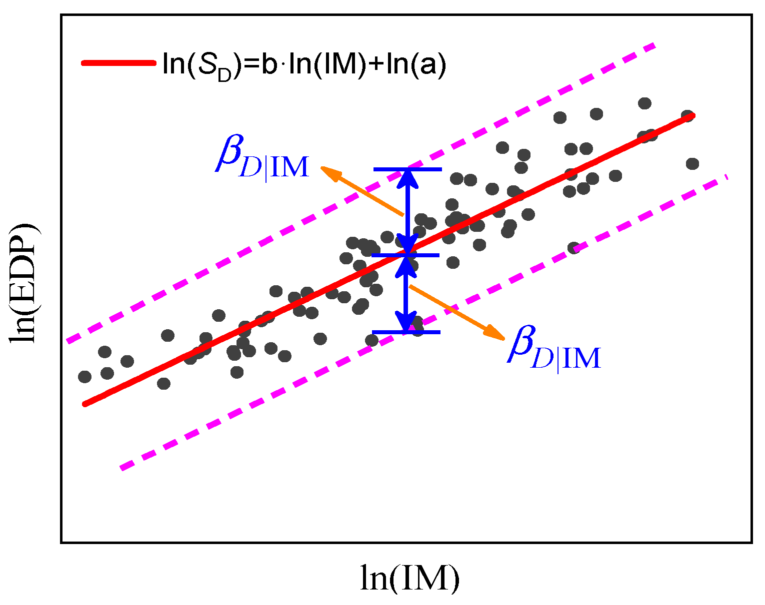
2. Probabilistic Seismic Demand Model
3. Evaluation Criteria for the Optimal Ground Motion IMs
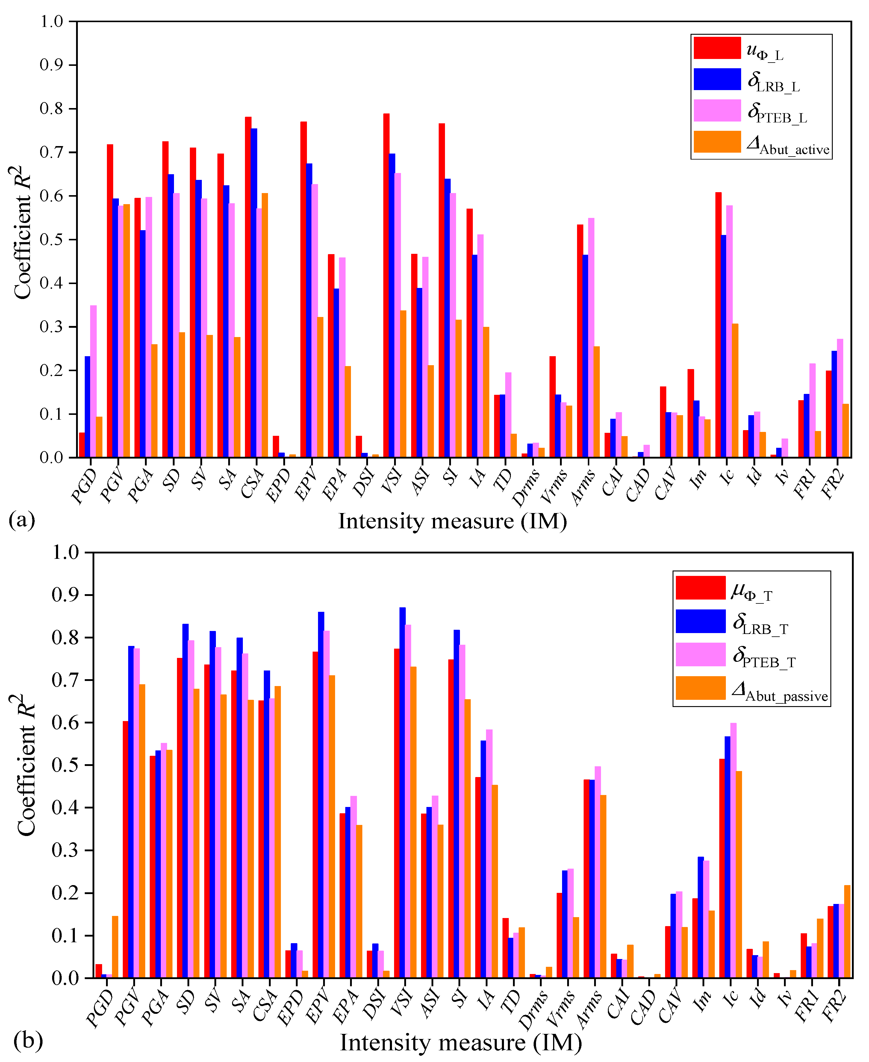
3.1. Efficiency
3.2. Practicality
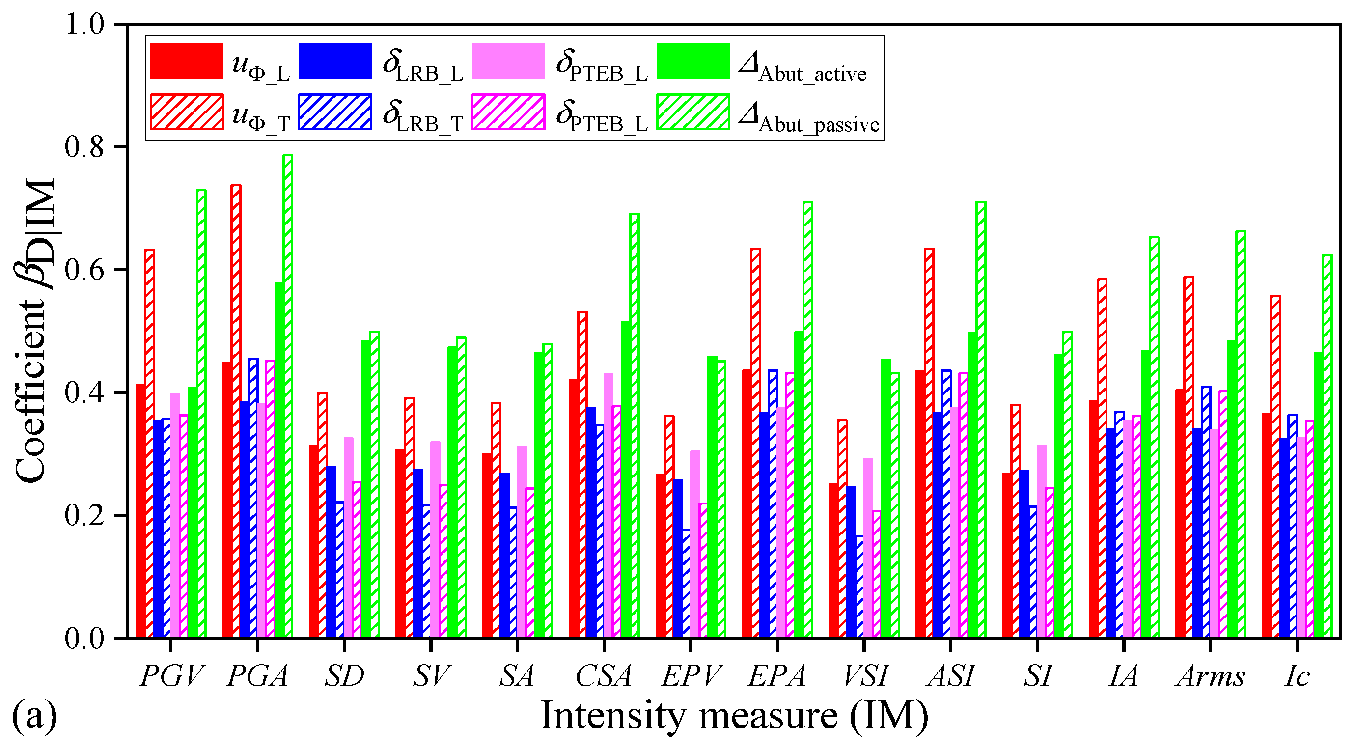
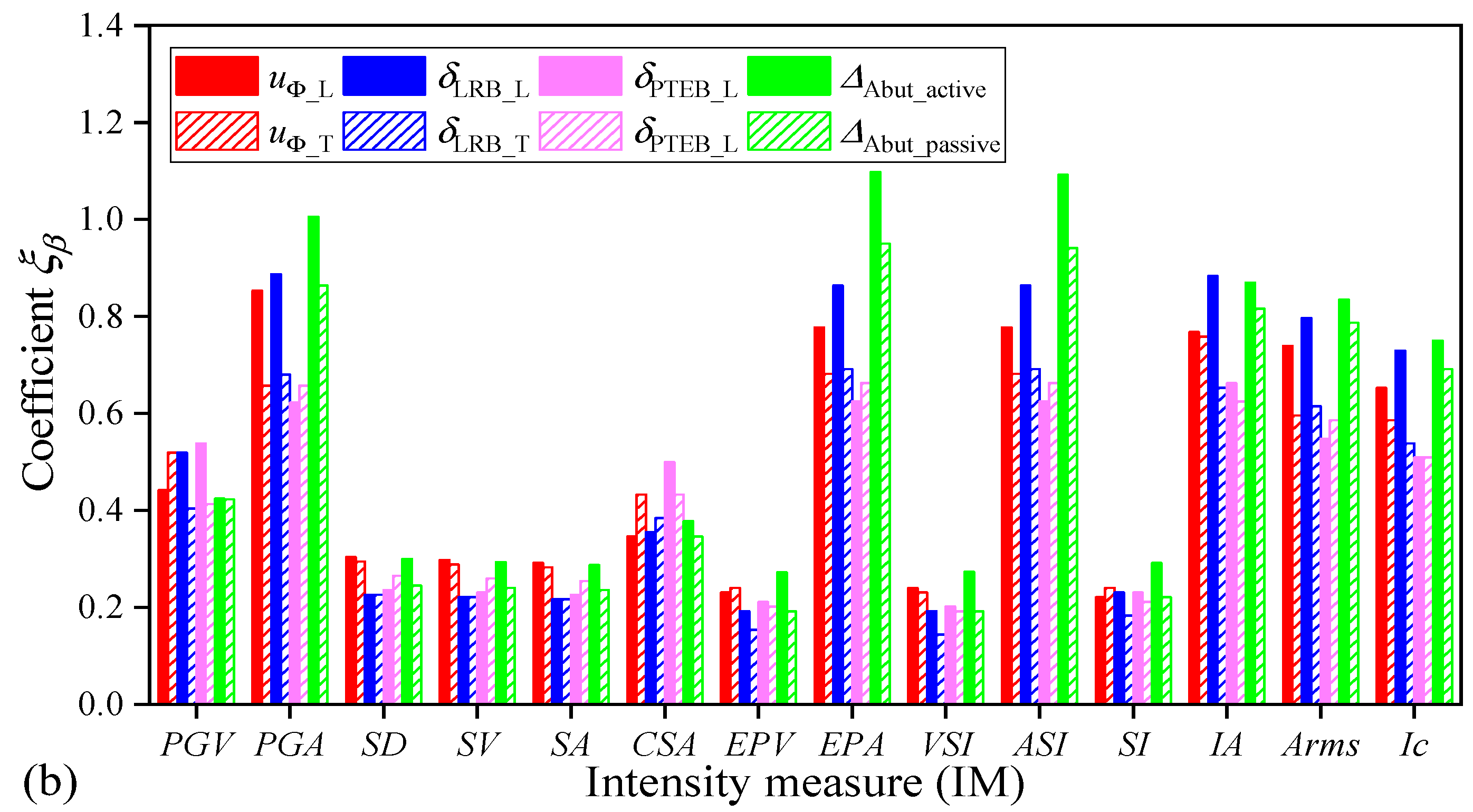
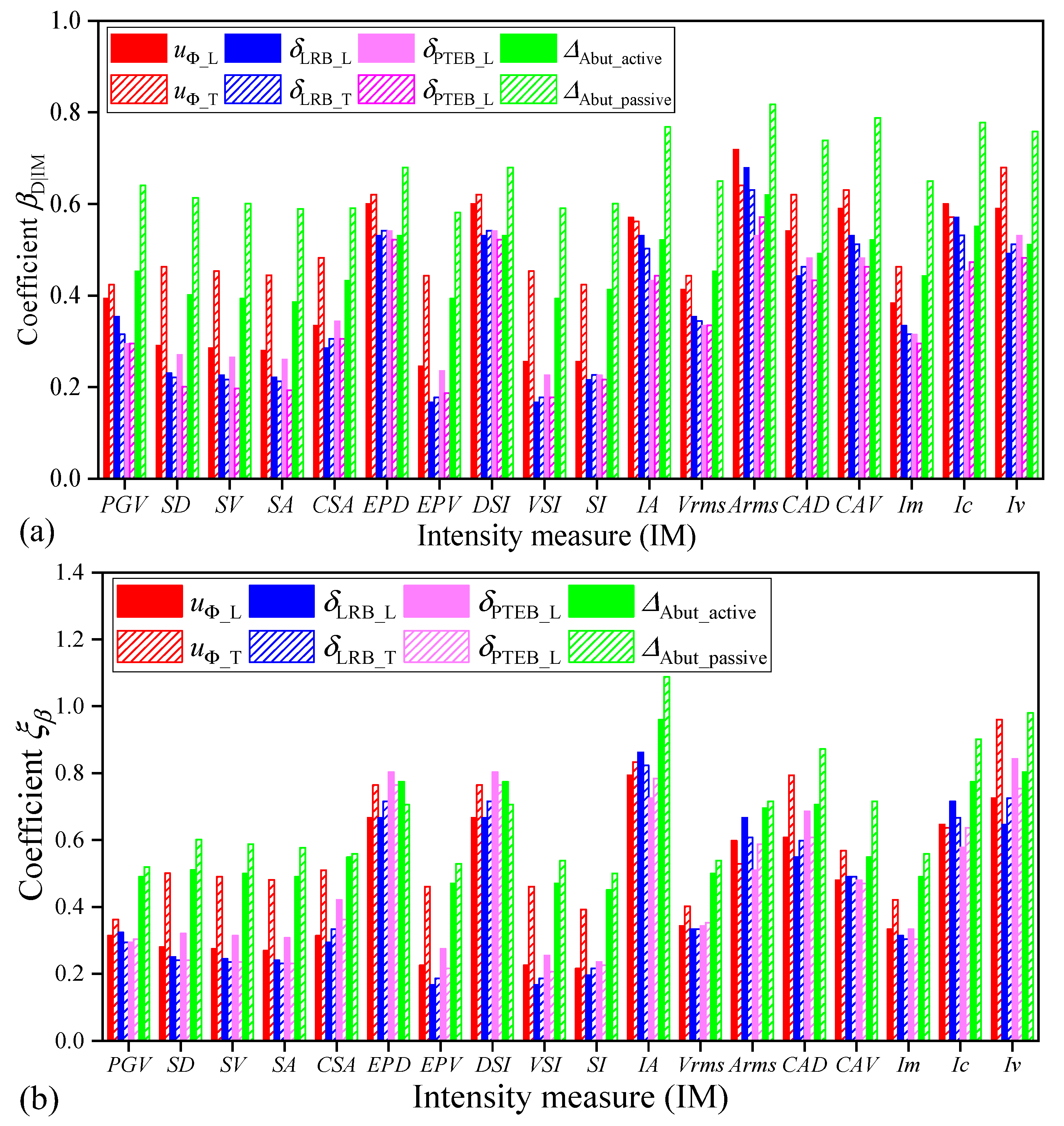
3.3. Proficiency
3.4. Sufficiency
3.5. Hazard Computability
4. Case Study: FE Modeling and Engineering Demand Parameters
4.1. Bridge Description and FE Modeling
4.2. Engineering Demand Parameters (EDPs)
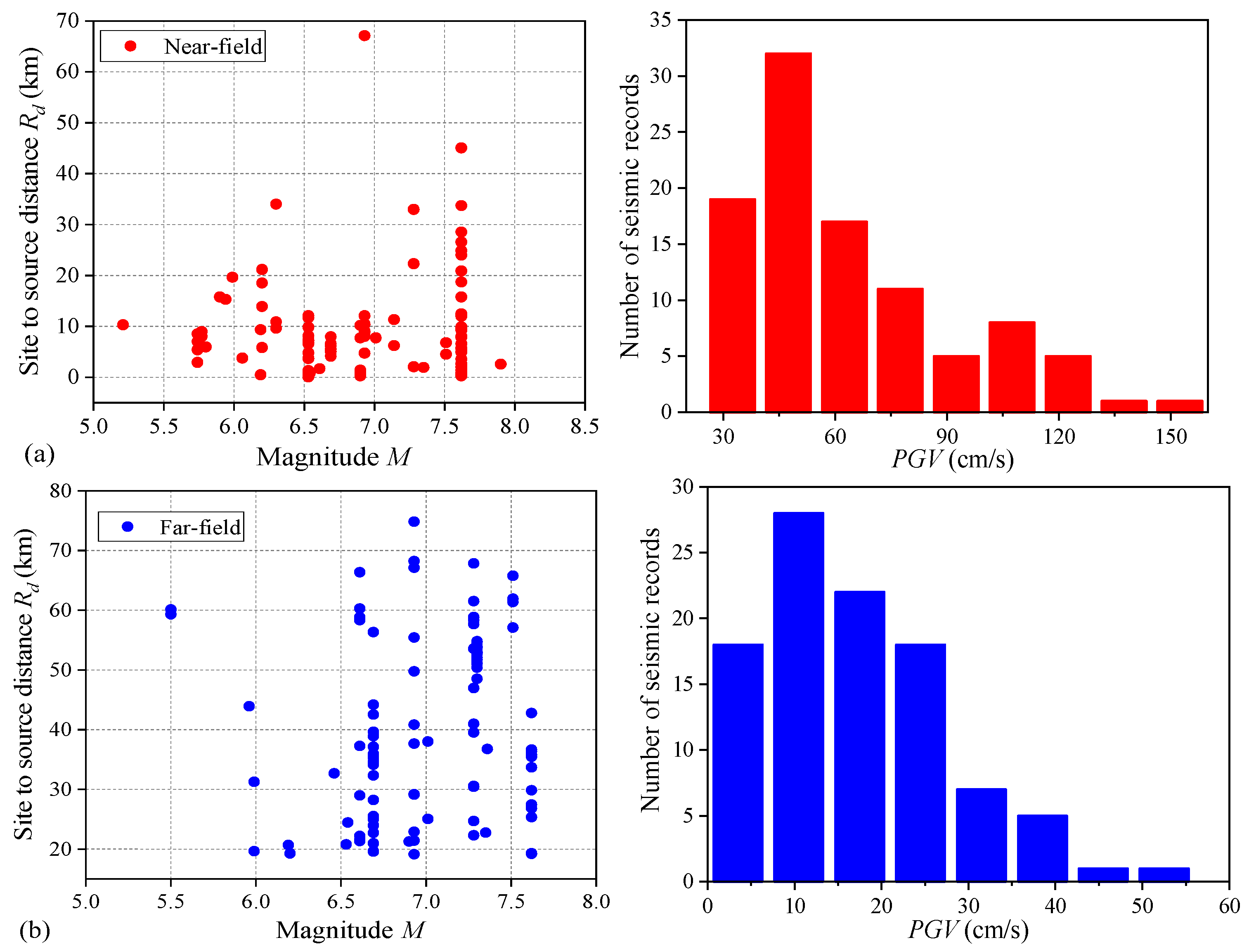
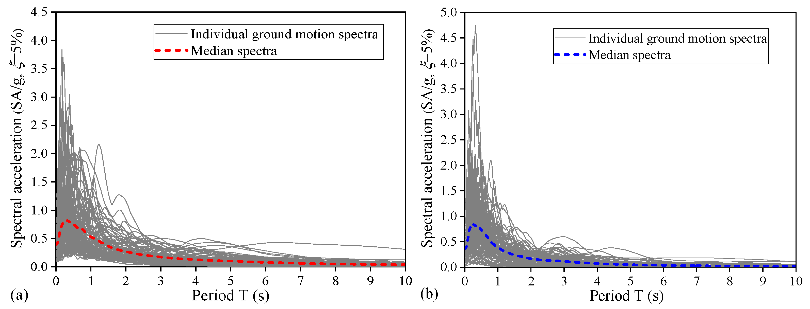
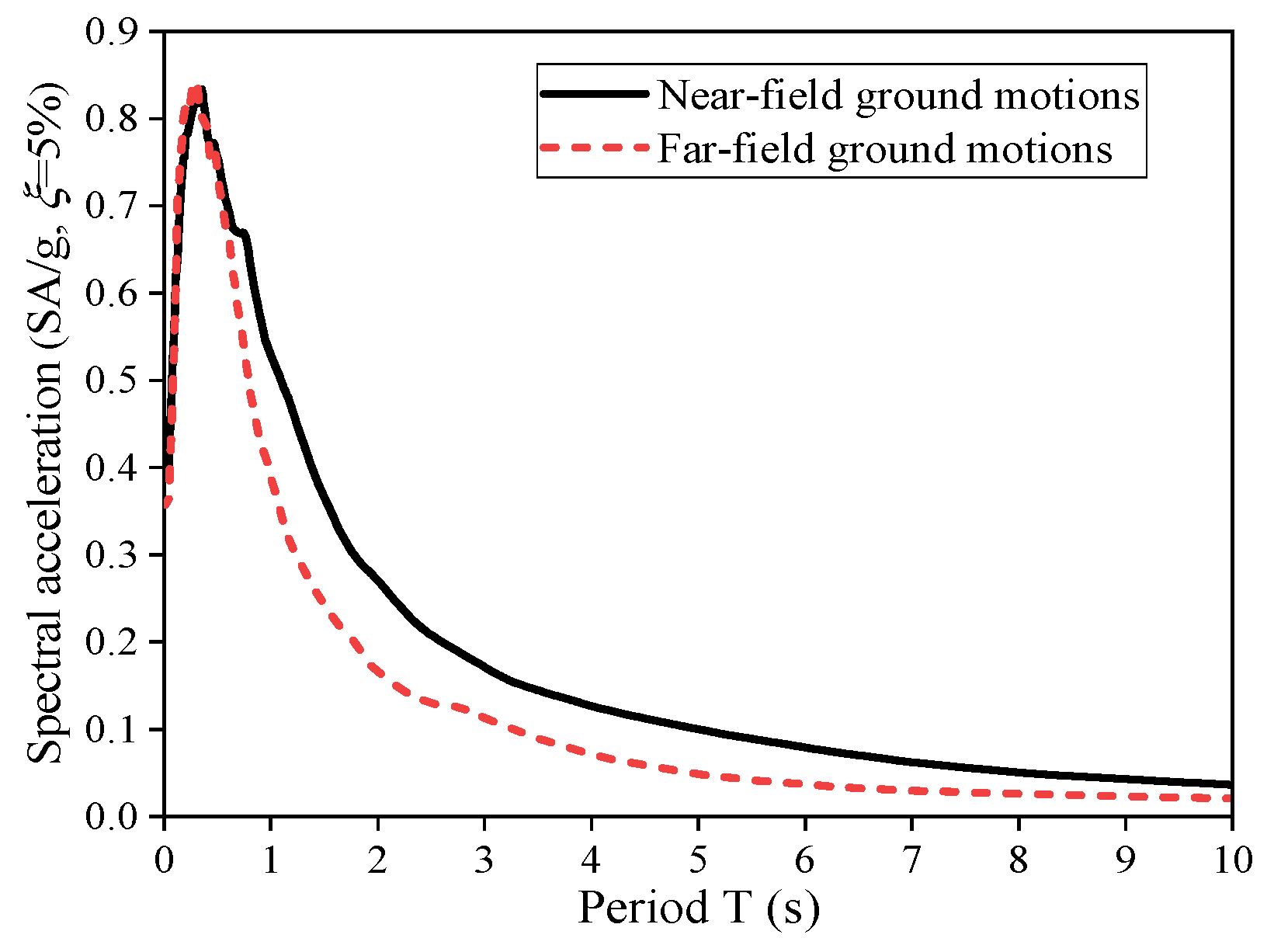
5. Ground Motion Records and the Considered Ground Motion IMs
6. Results and Discussions of the Selection of Ground Motion IMs
6.1. Selection of IMs for the Near-Field Ground Motions
6.2. Selection of IMs for the Far-Field Ground Motions
7. Effect of Uncertainties in Ground Motions on the PSDA of Highway Bridges
8. Conclusions
- (1)
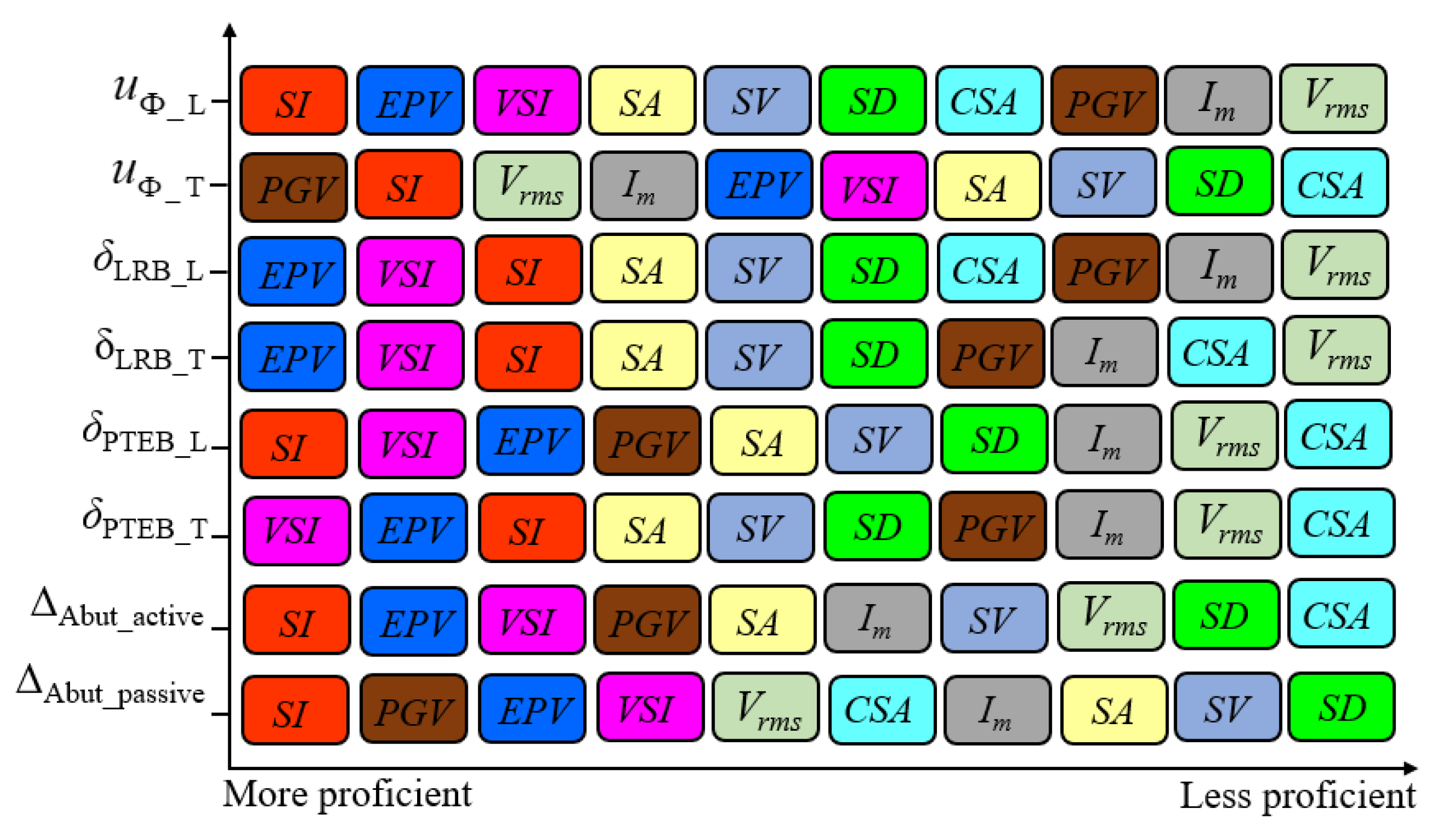
- IM efficiency is the most important criterion in reflecting the RTR variability of ground motions. For both the far-field and pulse-like ground motions, efficiency of the ground motion IMs that is related to structural form, spectrum-related ground motion IMs (i.e., SA and CSA), and velocity-based IMs (i.e., PGV and VSI) is good and helpful in reducing the RTR variability of ground motions. An efficient IM will reduce the influence of the RTR variability of ground motions in the predictions of structural demands.
- (2)
- Both the BTB and RTR variabilities of ground motions have important effects on the PSDA and the developed PSDMs of highway bridges. On the one hand, uncertainty stemming from the BTB variability of ground motions may lead to a significant difference in the developed PSDMs, so it is necessary to carefully select the input seismic records in the PSDA of highway bridges. On the other hand, for a given selected ground motion bin or database, uncertainty derived from the RTR variability of seismic records can also result in discreteness of the PSDMs.
Author Contributions
Funding
Institutional Review Board Statement
Informed Consent Statement
Data Availability Statement
Acknowledgments
Conflicts of Interest
References
- Moehle, J.; Deierlein, G.G. A framework methodology for performance-based earthquake engineering. Proceedings of 13th World Conference on Earthquake Engineering, Vancouver, BC, Canada, 1–6 August 2004. [Google Scholar]
- Khosravikia, F.; Clayton, P. Updated evaluation metrics for optimal intensity measure selection in probabilistic seismic demand models. Eng. Struct. 2020, 202, 109899. [Google Scholar] [CrossRef]
- Li, H.H.; Li, L.F. Bridge time-varying seismic fragility considering variables’ correlation. J. Vib Shock. 2019, 38, 173–183. (In Chinese) [Google Scholar]
- Li, H.H.; Li, L.F.; Wu, W.P.; Xu, L. Seismic fragility assessment framework for highway bridges based on an improved uniform design-response surface model methodology. Bull. Earthq. Eng. 2020, 18, 2329–2353. [Google Scholar] [CrossRef]
- Li, H.H.; Li, L.F.; Zhou, G.J.; Xu, L. Effects of various modeling uncertainty parameters on the seismic response and seismic fragility estimates of the aging highway bridges. Bull. Earthq. Eng. 2020, 18, 6337–6373. [Google Scholar] [CrossRef]
- Li, H.H.; Li, L.F.; Zhou, G.J.; Xu, L. Time-dependent seismic fragility assessment for aging highway bridges subject to non-uniform chloride-induced corrosion. J. Earthq. Eng. 2020, 24, 2020. [Google Scholar] [CrossRef]
- Li, H.H.; Li, L.F.; Xu, L. Seismic Response and Fragility Estimates of Highway Bridges Considering Various Modeling Uncertainty Parameters. In Proceedings of the Civil Infrastructures Confronting Severe Weathers and Climate Changes Conference, NanChang, China, 19–21 July2021; pp. 31–53. [Google Scholar]
- Giovenale, P.; Cornell, C.A.; Esteva, L. Comparing the adequacy of alternative ground motion intensity measures for the estimation of structural responses. Earthq. Eng. Struct. Dyn. 2004, 33, 951–979. [Google Scholar] [CrossRef]
- Luco, N.; Cornell, C.A. Structure-specific scalar intensity measures for near-source and ordinary earthquake ground motions. Earthq. Spectra. 2007, 23, 357–392. [Google Scholar] [CrossRef] [Green Version]
- Padgett, J.E.; Nielson, B.G.; DesRoches, R. Selection of optimal intensity measures in probabilistic seismic demand models of highway bridge portfolios. Earthq. Eng. Struct. Dyn. 2008, 37, 711–725. [Google Scholar] [CrossRef]
- Wu, W.P. Seismic Fragility of Reinforced Concrete Bridges with Consideration of Various Sources of Uncertainty. Ph.D. Thesis, Hunan University, Changsha, China, 2016. (In Chinese). [Google Scholar]
- Babaei, S.R.; Taghikhany, A.T.; Sharifi, M. Optimal ground motion intensity measure selection for probabilistic seismic demand modeling of fixed pile-founded offshore platforms. Ocean. Eng. 2021, 242, 110116. [Google Scholar] [CrossRef]
- Bradley, B.A.; Cubrinovski, M.; Dhakal, R.P.; Macrae, G.A. Intensity measures for the seismic response of pile foundations. Soil. Dyn. Earthq. Eng. 2009, 29, 1046–1058. [Google Scholar] [CrossRef] [Green Version]
- Wang, X.; Shafieezadeh, A.; Ye, A.J. Optimal intensity measures for probabilistic seismic demand modeling of extended pile-shaft-supported bridges in liquefied and laterally spreading ground. Bull. Earthq. Eng. 2018, 16, 229–257. [Google Scholar] [CrossRef]
- Padgett, J.E.; DesRoches, R. Sensitivity of seismic response and fragility to parameter uncertainty. J. Struct. Eng. 2007, 133, 1710–1718. [Google Scholar] [CrossRef] [Green Version]
- Padgett, J.E.; Ghosh, J.; Dueñas-Osorio, L. Effects of liquefiable soil and bridge modeling parameters on the seismic reliability of critical structural components. Struct. Infrastruct. Eng. 2010, 9, 59–77. [Google Scholar]
- Mangalathu, S.; Jeon, J.S. Critical uncertainty parameters influencing the seismic performance of bridges using Lasso regression. Earthq. Eng. Struct. Dyn. 2018, 47, 784–801. [Google Scholar] [CrossRef]
- Kiureghian, A.D.; Ditlevsen, O. Aleatory or epistemic? Does it matter? Struct. Saf. 2009, 31, 105–112. [Google Scholar] [CrossRef]
- Mackie, K.; Stojadinović, B. Seismic Demands for Performance-Based Design of Bridges; PEER 2003/16 Report; PEER Center: Berkeley, CA, USA, 2003. [Google Scholar]
- Cornell, C.A.; Jalayer, F.; Hamburger, R.; Foutch, D. Probabilistic basis for 2000 sac federal emergency management agency steel moment frame guidelines. J. Struct. Eng. 2002, 128, 526–533. [Google Scholar] [CrossRef] [Green Version]
- Chen, X. System fragility assessment of tall-pier bridges subjected to near-fault ground motions. J. Bridge Eng. 2020, 25, 04019143. [Google Scholar] [CrossRef]
- Wu, W.P.; Li, L.F.; Shao, X.D. Seismic assessment of medium-span concrete cable-stayed bridge using the component and system fragility functions. J. Bridge Eng. 2016, 21, 04016027. [Google Scholar] [CrossRef]
- Cornell, C.A. Hazard, ground-motions and probabilistic assessment for PBSD. In Performance Based Seismic Design Concepts and Implementation; PEER Report; PEER Center: Berkeley, CA, USA, 2004. [Google Scholar]
- Mackie, K.; Stojadinović, B. Probabilistic seismic demand model for California highway bridges. J. Bridge Eng. 2001, 6, 468–481. [Google Scholar] [CrossRef] [Green Version]
- Mollaioli, F.; Lucchini, A.; Cheng, Y.; Monti, G. Intensity measures for the seismic response prediction of base-isolated buildings. Bull. Earthq. Eng. 2013, 11, 1841–1866. [Google Scholar] [CrossRef]
- Fisher, R.A. Statistical Methods for Research Workers; Oliver and Boyd: Edinburgh, UK, 1925. [Google Scholar]
- Tang, W.H.; Ang, A. Probability Concepts in Engineering: Emphasis on Applications to Civil and Environmental Engineering, 2nd ed.; Wiley: Hoboken, NJ, USA, 2007. [Google Scholar]
- Wasserstein, R.L.; Lazar, N.A. The ASA statement on p-values: Context, process, and purpose. Am. Stat. 2016, 70, 129–133. [Google Scholar] [CrossRef] [Green Version]
- Tothong, P.; Cornell, C.A. Probabilistic Seismic Demand Analysis Using Advanced Ground Motion Intensity Measures, Attenuation Relationships, and Near-Fault Effects; Technical Report; Pacific Earthquake Engineering Research Center, University of California: Berkeley, CA, USA, 2006. [Google Scholar]
- Iervolino, I.; Manfredi, G. A review of ground motion record selection strategies for dynamic structural analysis. In Modern Testing Techniques for Structural Systems; Bursi, O.S., Wagg, D., Eds.; CISM International Centre for Mechanical Sciences; Springer: Vienna, Austria, 2008. [Google Scholar]
- Ministry of Communications of PRC. Guidelines for Seismic Design of Highway Bridges (JTG/TB02-01); China Communications Press: Beijing, China, 2008. (In Chinese) [Google Scholar]
- Manual, O. Open system for Earthquake Engineering Simulation User Command-Language Manual; Pacific Earthquake Engineering Research Center, University of California: Berkeley, CA, USA, 2009. [Google Scholar]
- Shome, N.; Cornell, C.A.; Bazzurro, P.; Caraballo, J.E. Earthquakes, records, and nonlinear responses. Earthq. Spectra. 1998, 14, 467–500. [Google Scholar] [CrossRef]
- PEER (Pacific Earthquake Engineering Research Center). PEER Ground Motion Database; PEER (Pacific Earthquake Engineering Research Center): Berkeley, CA, USA, 2015. [Google Scholar]


| Parameters | Description | Value | Units | |
|---|---|---|---|---|
| Structure-related parameters | λw | Concrete weight coefficient | 1.04 | — |
| D | Pier diameter | 1.4 | m | |
| c | Concrete cover thickness | 0.05 | m | |
| φ | Longitudinal reinforcement diameter | 28 | mm | |
| ξ | Damping ratio | 0.05 | — | |
| Material-related parameters | Ec | Young’s modulus of concrete | 3 × 10⁴ | MPa |
| fc, cover | The peak strength of cover concrete | 27.58 | MPa | |
| εc,cover | Peak strain of cover concrete | 0.002 | — | |
| εcu,cover | The ultimate strain of cover concrete | 0.006 | — | |
| fc, core | The peak strength of core concrete | 34.47 | MPa | |
| εc,core | Peak strain of core concrete | 0.005 | 0.005 | |
| εcu,core | The ultimate strain of core concrete | 0.02 | 0.02 | |
| Es | Young’s modulus of steel rebar | 2 × 10⁵ | MPa | |
| fy | Yield strength of steel rebar | 335 | MPa | |
| γ | Post-yield to initial stiffness ratio | 0.02 | — | |
| Boundary condition-related parameters | μPETB | The friction coefficient of PTEB | 0.15 | — |
| GPETB | Shear modulus of PTEB | 1180 | MPa | |
| KP_LRB | Post-yield stiffness of LRB | 1500 | kN/m | |
| Pult | Abutment ultimate capacity | 10,853 | kN | |
| Kpassive | Abutment passive stiffness | 3.04 × 10⁵ | kN/m | |
| Kactive | Abutment active stiffness | 1.86 × 10⁴ | kN/m | |
| Keff | Pounding effective stiffness | 1.94 × 10⁶ | kN/m |
| ID | EDP | Abbreviation | Unit | Note |
|---|---|---|---|---|
| 1 | Curvature ductility of the pier | m−1 | Longitudinal | |
| 2 | The curvature ductility of the pier | m−1 | Transverse | |
| 3 | Relative displacement of the LRB | δLRB_L | cm | Longitudinal |
| 4 | Relative displacement of the LRB | δLRB_T | cm | Transverse |
| 5 | Relative displacement of the PTEB | δPTEB_L | cm | Longitudinal |
| 6 | Relative displacement of the PTEB | δPTEB_T | cm | Transverse |
| 7 | Abutment deformation | ΔAbut_active | cm | Active |
| 8 | Abutment deformation | ΔAbut_passive | cm | Passive |
| IM Number | IM Name | Definition | Calculation Method | Unit |
|---|---|---|---|---|
| 1 | PGD | Peak ground displacement | cm | |
| 2 | PGV | Peak ground velocity | cm/s | |
| 3 | PGA | Peak ground acceleration | g | |
| 4 | SD | Spectra displacement | cm | |
| 5 | SV | Spectral velocity | cm/s | |
| 6 | SA | Spectral acceleration | g | |
| 7 | CSA | Cordova spectral acceleration | cm/s2 | |
| 8 | EPD | Effective peak displacement | cm | |
| 9 | EPV | Effective peak velocity | cm/s | |
| 10 | EPA | Effective peak acceleration | cm/s2 | |
| 11 | DSI | Displacement response intensity | cm | |
| 12 | VSI | Displacement velocity intensity | cm/s | |
| 13 | ASI | Acceleration velocity intensity | g | |
| 14 | SI | Response spectrum intensity | cm | |
| 15 | IA | Arias intensity | cm/s | |
| 16 | TD | Strong motion duration | s | |
| 17 | Drms | Root mean square displacement | cm | |
| 18 | Vrms | Root mean square velocity | cm/s | |
| 19 | Arms | Root mean square acceleration | cm/s2 | |
| 20 | CAI | Cumulative absolute impulse | cm-s | |
| 21 | CAD | Cumulative absolute displacement | cm | |
| 22 | CAV | Cumulative absolute velocity | cm/s | |
| 23 | Im | Median period intensity measure | cm/s0.75 | |
| 24 | IC | Characteristic intensity | cm1.5/s2.5 | |
| 25 | ID | Displacement intensity | cm-s | |
| 26 | IV | Velocity intensity | cm | |
| 27 | FR1 | Frequency ratio 1 | s | |
| 28 | FR2 | Frequency ratio 2 | s |
| IM | δLRB_L | δLRB_T | δPTEB_L | δPTEB_T | ΔAbut_active | ΔAbut_passive | ||
|---|---|---|---|---|---|---|---|---|
| PGV | 0.000 | 0.000 | 0.000 | 0.000 | 0.000 | 0.000 | 0.048 | 0.000 |
| SA | 0.182 | 0.000 | 0.038 | 0.038 | 0.000 | 0.067 | 0.490 | 0.806 |
| CSA | 0.000 | 0.000 | 0.000 | 0.000 | 0.000 | 0.000 | 0.048 | 0.000 |
| EPV | 0.077 | 0.000 | 0.010 | 0.000 | 0.000 | 0.019 | 0.614 | 0.883 |
| VSI | 0.173 | 0.000 | 0.038 | 0.106 | 0.000 | 0.048 | 0.442 | 0.672 |
| SI | 0.288 | 0.005 | 0.154 | 0.096 | 0.086 | 0.144 | 0.403 | 0.538 |
| IM | δLRB_L | δLRB_T | δPTEB_L | δPTEB_T | ΔAbut_active | ΔAbut_passive | ||
|---|---|---|---|---|---|---|---|---|
| PGV | 0.038 | 0.125 | 0.067 | 0.086 | 0.125 | 0.096 | 0.566 | 0.566 |
| SA | 0.269 | 0.230 | 0.490 | 0.365 | 0.816 | 0.346 | 0.528 | 0.326 |
| CSA | 0.048 | 0.019 | 0.058 | 0.038 | 0.096 | 0.038 | 0.634 | 0.614 |
| EPV | 0.269 | 0.202 | 0.422 | 0.336 | 0.912 | 0.326 | 0.595 | 0.269 |
| VSI | 0.250 | 0.192 | 0.384 | 0.317 | 0.893 | 0.326 | 0.634 | 0.307 |
| SI | 0.173 | 0.125 | 0.211 | 0.182 | 0.614 | 0.192 | 0.950 | 0.682 |
| IM | δLRB_L | δLRB_T | δPTEB_L | δPTEB_T | ΔAbut_active | ΔAbut_passive | ||
|---|---|---|---|---|---|---|---|---|
| PGV | 0.571 | 0.483 | 0.699 | 0.798 | 0.808 | 0.837 | 0.699 | 0.798 |
| SA | 0.955 | 0.483 | 0.680 | 0.630 | 0.571 | 0.561 | 0.335 | 0.973 |
| CSA | 0.660 | 0.690 | 0.424 | 0.552 | 0.601 | 0.630 | 0.315 | 0.719 |
| EPV | 0.808 | 0.384 | 0.660 | 0.739 | 0.640 | 0.749 | 0.384 | 0.965 |
| VSI | 0.640 | 0.325 | 0.867 | 0.916 | 0.729 | 0.906 | 0.443 | 0.887 |
| SI | 0.335 | 0.236 | 0.532 | 0.532 | 0.926 | 0.581 | 0.680 | 0.719 |
| Vrms | 0.512 | 0.414 | 0.670 | 0.670 | 0.955 | 0.670 | 0.670 | 0.739 |
| Im | 0.532 | 0.916 | 0.355 | 0.315 | 0.217 | 0.286 | 0.217 | 0.798 |
| IM | δLRB_L | δLRB_T | δPTEB_L | δPTEB_T | ΔAbut_active | ΔAbut_passive | ||
|---|---|---|---|---|---|---|---|---|
| PGV | 0.176 | 0.598 | 0.323 | 0.941 | 0.862 | 0.794 | 0.647 | 0.539 |
| SA | 0.951 | 0.372 | 0.588 | 0.137 | 0.108 | 0.167 | 0.686 | 0.921 |
| CSA | 0.637 | 0.059 | 0.372 | 0.049 | 0.108 | 0.098 | 0.539 | 0.804 |
| EPV | 0.412 | 0.176 | 0.627 | 0.147 | 0.294 | 0.294 | 0.976 | 0.804 |
| VSI | 0.363 | 0.196 | 0.539 | 0.176 | 0.323 | 0.333 | 0.970 | 0.794 |
| SI | 0.137 | 0.314 | 0.284 | 0.578 | 0.657 | 0.764 | 0.804 | 0.657 |
| Vrms | 0.127 | 0.764 | 0.206 | 0.764 | 0.715 | 0.676 | 0.529 | 0.470 |
| Im | 0.588 | 0.235 | 0.813 | 0.402 | 0.451 | 0.519 | 0.970 | 0.843 |
| Ground Motions | (i) Efficiency; (ii) Practicality; and (iii) Proficiency Evaluation | (iv) Sufficiency Evaluation | |
|---|---|---|---|
| Magnitude (M) | Source-to-Site Distance (Rd) | ||
| Near-field | SA, SV, SD, CSA, PGV, EPV, VSI, and SI. | (1) The optimal IM varies for different bridge EDPs. (2) All of the eight considered IMs do not satisfy sufficiency requirement for M. | (1) The optimal IM varies for different bridge EDPs. (2) All of the eight considered IMs except CSA satisfy the sufficiency requirement for Rd. |
| Far-field | SA, SV, SD, CSA, PGV, EPV, VSI, SI, Vrms, and Im. | (1) The optimal IM varies for different bridge EDPs. (2) All of the ten considered IMs satisfy the sufficiency requirement for M. | |
Publisher’s Note: MDPI stays neutral with regard to jurisdictional claims in published maps and institutional affiliations. |
© 2022 by the authors. Licensee MDPI, Basel, Switzerland. This article is an open access article distributed under the terms and conditions of the Creative Commons Attribution (CC BY) license (https://creativecommons.org/licenses/by/4.0/).
Share and Cite
Li, H.; Zhou, G.; Wang, J. Selection of Ground Motion Intensity Measures and Evaluation of the Ground Motion-Related Uncertainties in the Probabilistic Seismic Demand Analysis of Highway Bridges. Buildings 2022, 12, 1184. https://doi.org/10.3390/buildings12081184
Li H, Zhou G, Wang J. Selection of Ground Motion Intensity Measures and Evaluation of the Ground Motion-Related Uncertainties in the Probabilistic Seismic Demand Analysis of Highway Bridges. Buildings. 2022; 12(8):1184. https://doi.org/10.3390/buildings12081184
Chicago/Turabian StyleLi, Huihui, Guojie Zhou, and Jun Wang. 2022. "Selection of Ground Motion Intensity Measures and Evaluation of the Ground Motion-Related Uncertainties in the Probabilistic Seismic Demand Analysis of Highway Bridges" Buildings 12, no. 8: 1184. https://doi.org/10.3390/buildings12081184