Evaluation of Inverted-Pendulum-with-Rigid-Legs Walking Locomotion Models for Civil Engineering Applications

Abstract

Bipedal models for walkers, originally developed in the research field of biomechanics, have been identified as potential candidates for modelling pedestrians in structural engineering applications. These models provide insight into both the kinetics and kinematics of walking locomotion and are considered to have a significant potential to improve the vibration serviceability assessment of civil engineering structures. Despite this notion, the ability of the bipedal models to represent the key features of the walking gait and natural variability within the pedestrian population are still under-researched. This paper critically evaluates the performance of two bipedal models with rigid legs to realistically both reproduce key features of an individual pedestrian’s walking gait and represent a wide range of individuals. The evaluation is performed for walking on a rigid, rather than vibrating, structure due to the availability of experimental data and expectation that successful modelling on rigid surfaces is a necessary condition for progressing towards modelling on the vibrating structures. Ready-to-use equations are provided and the ability of the models to represent the kinematics and kinetics of individual pedestrians as well as the inter-subject variability typical of the human population is critically evaluated. It was found that the two models could generate realistic combinations of the gait parameters and their correlations, but are less successful in reproducing genuine kinetic and kinematics profiles.

1. Introduction

It is more than four decades since the first design guidance for the vibration serviceability assessment of footbridges, BS5400, was developed in 1978 [1] in recognition of the need to evaluate the structural vibration response to dynamic excitation induced by pedestrians. A pedestrian was modelled as a harmonic force moving across the bridge at a constant speed and at a “pacing” (also called “step”) frequency matching a natural frequency of the structure. This single-pedestrian-exciting-the-resonance loading scenario has been at the heart of the vibration serviceability assessment of footbridges for almost three decades. A gradual introduction of high-strength and light-weight materials in contemporary structural design has resulted in new footbridges that are usually more slender, lighter, and less damped, and, therefore, more sensitive to dynamic loading than their older counterparts. As a consequence, there is a need for an improved modelling of pedestrian loading that exists. Some refinements, such as the inclusion of multi-pedestrian loading scenarios and the consideration of inter-subject variability in the pacing rate within a pedestrian crowd, have already been introduced in the new generation of design guidelines [2,3,4]. Research into stochastic models for pedestrian-induced force have been advanced from those that account for variations in the pacing rate within a pedestrian population [5] towards the inclusion of the probability distributions of pedestrian mass, dynamic force amplitude, and walking speed [6,7,8]. In addition, a detailed modelling of intra-subject (i.e., step-by-step) variations in pedestrian locomotion parameters is also available [6,9]. These relatively recent developments are underpinning the shift from a deterministic towards a probabilistic assessment of the vibration serviceability limit state of the structure. Nevertheless, the currently available models are limited to the structures on which pedestrians (and, therefore, the resulting dynamic forces) do not interact with the oscillating structure. The interaction term in this paper refers to the pedestrian–structure feedback loop, in which the structural vibration forces pedestrians to alter their walking locomotion which, in turn, alters the vibration response of the structure.

The excessive sway of the Millennium Bridge in London in June 2000, caused by a crowd of walkers, exposed a weakness in the design procedures that did not envisage the possibility of pedestrians interacting with the vibrating bridge deck [10]. The Millennium Bridge problem highlighted the need to understand the interaction mechanism and served as a motivation for developing more sophisticated models of pedestrians. An extensive experimental and theoretical line of research demonstrated that the structural behaviour could be explained by pedestrians continuously adjusting their placement of the foot on the moving deck to preserve their balance [11,12,13]. There is also some evidence that people might respond to deck vibration by synchronising with it [10,14]. In both cases, it has been acknowledged that pedestrians act as adaptable systems, highlighting the need for developing models that can genuinely represent pedestrian’s walking on vibrating structures [15]. Similar detailed studies of walking gait are required for developing and understanding the human–structure interaction in the vertical direction of vibration [16,17,18,19,20]. The vertical component of the human-induced dynamic force will be the focus of this paper.

A number of researchers have identified that bipedal models for walkers, originally developed in the research fields of biomechanics and robotics, can qualitatively describe the pedestrian–structure interaction. These models include both a simple inverted pendulum model with rigid legs [13,16,17,21] and more complex bipedal models with deformable and damped legs [22,23,24]. While the initial studies show the potential of the bipedal models to be used in structural engineering applications, there is a need for a more detailed insight into the performance of these models, especially in terms of their ability to cover relevant parameter space and genuinely represent inherent variability in the pedestrian population. This is important for the accurate modelling of individuals to both study an emerging crowd behaviour [25] and the pedestrian–structure interaction. An overview of the governing equations for these models, relatively new to the structural engineering community, is also required to facilitate wider validation of the models.

The aim of this paper is to provide a reference source for the two simplest inverted pendulum models of the vertical force and evaluate their performance on rigid level ground surfaces. The evaluation will focus on the ability of the models to generate walking locomotion parameters observed in practice. The study concentrates on rigid level surfaces due to the availability of experimental data that can be used for the evaluation of the models, and due to the expectation that a satisfactory performance of the bipedal models on the rigid surface is a necessary condition for these models to be considered as good candidates for modelling walking on vibrating structures. To achieve the main aim, the paper also explains the human walking locomotion process. This is done by transferring knowledge from medical and biomechanics research areas and presenting it in the context relevant for civil engineering applications to enable the evaluation of the bipedal models not only in this paper, but also those to be published in the future.

The paper starts with describing the kinematic and kinetic features of the walking gait. It then proceeds towards a detailed evaluation of the performance of the two bipedal models with rigid legs: the inverted pendulum model (IPM) and inverted pendulum with rocker foot model (IPRFM). The discussion of the findings and their relevance to modelling pedestrians on vibrating structures are then presented and conclusions are briefly summarised.

2. Characteristics of Walking Locomotion

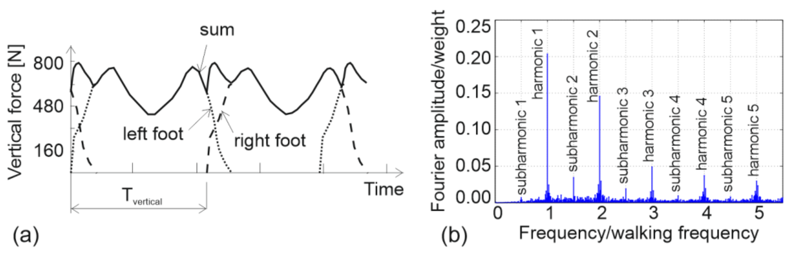
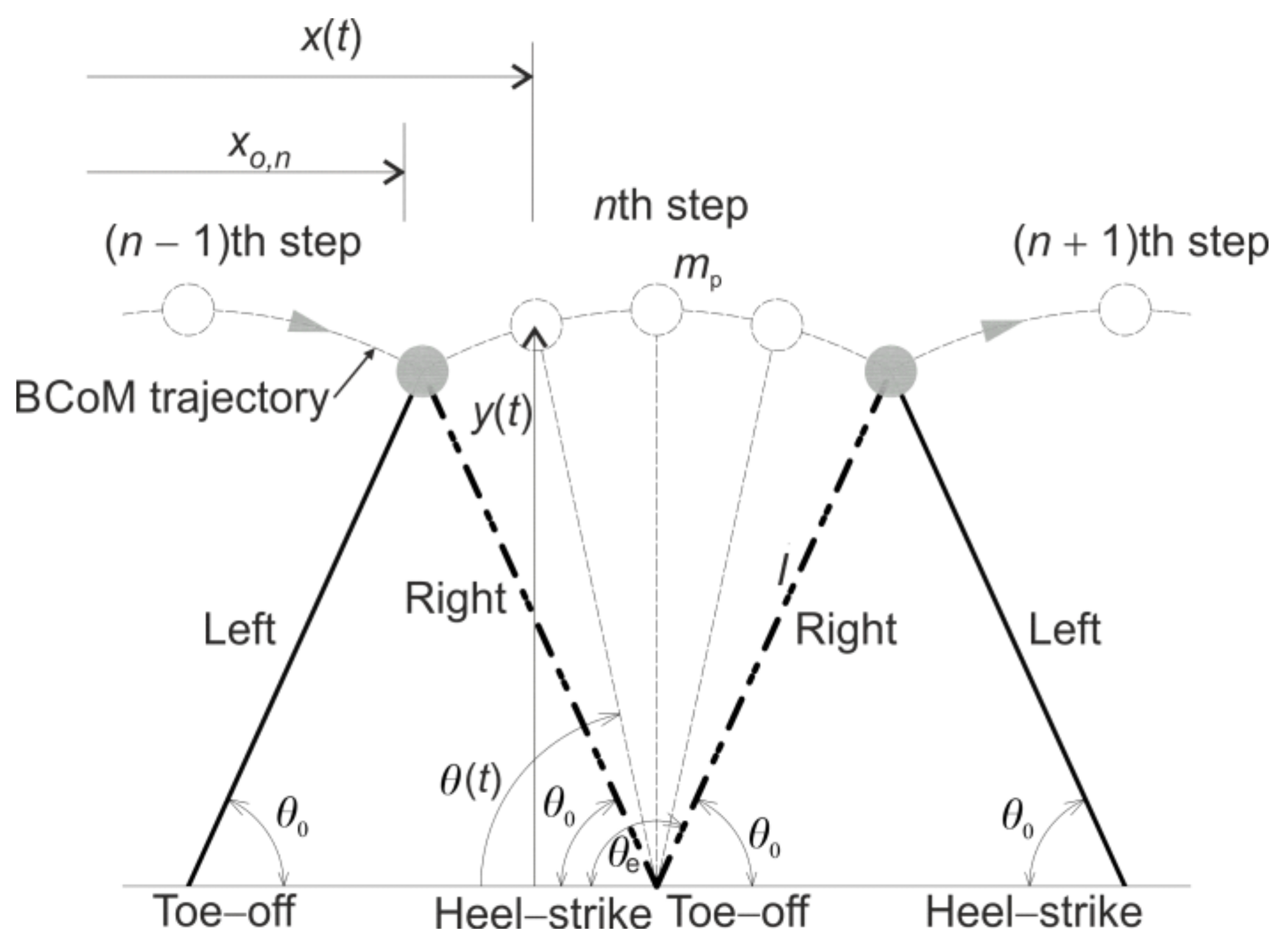
2.1. Kinematics and Kinetics of a Walking Gait Cycle

Gait analysis is a systematic study of the walking locomotion [26]. Traditionally, it is the ground reaction force (GRF) generated whilst walking that has been of most interest in structural engineering applications. This section, however, aims to describe not only the development of the force throughout a typical gait cycle (GC), but also the corresponding reference actions of the walker (e.g., heel-strike, toe-off, and other gait events) and the kinematics of the body centre of mass (BCoM). A GC is a cycle between two of the same nominal gait events of the same foot [27], such as the heel strike events of the right foot shown in Figure 1. Hence, a GC consists of two consecutive steps. Letters “R” and “L” in the figure refer to the right and left foot, respectively.

The human body in a walking posture is composed of a passenger unit and a locomotor unit [28]. The passenger unit consists of the upper body segments, which include head, arms, and trunk. These segments are carried by the lower body and they represent a passive contributor to the walking process. The locomotor unit, consisting of thighs, shanks, and feet, generates the body movement. Consequently, all gait events in a GC are usually described with reference to the positioning of the lower body parts, in particular, the two feet.

A GC consists of a stance and a swing phase of each leg (Figure 1). The stance phase is represented by the continuous contact of a leg with the ground, while the swing refers to the airborne phase of a leg. Besides the stance and swing phases, a GC can also be divided into a single support phase (SSP), when one foot only is in the contact with the ground, and double support phase (DSP), when both feet are simultaneously in the contact with the ground (Figure 1). SSP and DSP each occur twice in a GC.

Ayyappa [29], and Perry and Burnfield [28] have provided detailed descriptions of the walking phases and functions of body segments’ joints. Key information from their work will be summarised here, with frequent cross-referencing to Figure 1. Assuming the heel strike of the right leg is adopted as the reference event, the GC can be said to start with the DSP and, at the same time, the right stance phase. The right foot makes an initial contact (IC, 0–2%, where the two percentage values refer to the typical start time and the end time, respectively, relative to the GC duration), during which the right knee is close to full extension and the leg is nearly straight. The abrupt impact of the foot generates a short-lasting peak in the time history of the GRF (the heel strike transient in Figure 1) and the body weight starts to be transferred to the ground through the right heel.

After the IC, the GRF time history enters the loading response phase (LR, 2–12%). During LR, the rapid transfer of the body weight to the right leg hinders the extended posture of the knee, and the knee starts to flex. As a result, the BCoM starts to descend, reaching the minimum elevation approximately half way through the LR/DSP (Figure 1). The bony segment between the heel and the ankle joint (also known as the heel rocker) of the right foot acts as a lever arm, in which the forward momentum of the leg drives the forefoot to the ground. The GRF builds up along with an increase of the contact area of the right foot. On the contrary, the left foot prepares to lift off by pushing against the ground and propelling the pedestrian forward. The push of the left foot increases the BCoM’s elevation in the second half of the DSP (Figure 1). By the end of the LR, the GRF of the right leg reaches the first peak at F₁, while the force induced by the left leg decreases to zero, and the BCoM is at nominally the same elevation as at the beginning of the DSP. Meanwhile, the right knee is at the maximum flexion and the right foot is approximately in full contact with the ground. The DSP ends with the toe-off event of the left leg and the GC enters the SSP (Figure 1).

Figure 1. Ground reaction force, trajectory of body centre of mass, and key events in a gait cycle (adapted from [27]).

Figure 1. Ground reaction force, trajectory of body centre of mass, and key events in a gait cycle (adapted from [27]).

In the SSP (12–50%), only the right leg is in contact with the ground, while the left leg enters the swing phase. As soon as the left foot loses contact with the ground, the time history of the GRF only consists of the right leg’s reaction (Figure 1). The first part of this SSP, during which the right foot is relatively stationary, is called the mid-stance (MSt, 12–30%). Due to the forward momentum, the body moves in front of the ankle joint axis (often referred to as the ankle rocker). At the same time, the knee-flexion keeps decreasing since the stability during the stance phase is at its optimum when the knee is in full extension. The swinging momentum of the left leg also plays a role in extending the right knee. As a consequence of the knee’s extension, the BCoM’s elevation continues to increase. On the contrary, the amplitude of the GRF decreases because of the upward momentum of the swinging leg. By the end of the MSt, the magnitude of GRF descends to its lowest point, F₂, while the BCoM reaches its maximum elevation (Figure 1). Once the swinging left leg becomes the leading leg (by overtaking the right leg), the left knee extends rapidly, allowing the pedestrian to achieve a certain step length.

After the MSt, the GC enters the terminal stance (TSt, 30–50%) that is initiated by the heel rise of the right foot. The TSt completes the SSP of the right leg and the swing phase of the left leg. The entire body makes a forward fall over the bony segment of the forefoot, acting as the forefoot rocker. The right knee reaches the state of full extension that makes the falling-forward movement of the BCoM relatively similar to the trajectory of an inverted pendulum. To prepare for the stance phase of the left leg, the left knee is in full extension. By the end of the TSt, the GRF of the right leg reaches the second peak at F₃. The TSt ends when the swing leg makes first contact with the ground. The SSP ends and the GC enters the second DSP.

Right after the TSt is the pre-swing (PS, 50–62%) phase of the right leg. This phase occurs at the same time as the IC and the LR of the left leg, and therefore, the BCoM experiences a similar trajectory pattern, as explained earlier in relation to the IC and LR phases of the right leg. The body weight is transferred from the right leg to the left leg, resulting in the rapid decrease of the GRF for the right and increase for the left leg (Figure 1). To prepare for the swing phase, the right knee experiences significant flexion. Meanwhile, the right foot pushes the ground through metatarsal heads and toes (known as toe rocker) to progress the limb forward. The pre-swing phase ends with the toe-off event, which is also the terminal event of the stance phase of the right leg. The rest of the GC (62–100%) is the SSP of the left leg (and the swing phase of the right leg). The GC ends with the heel strike event of the right foot.

During a GC, the forward velocity is lowest when the BCoM is at its highest position, at around midstance [30], while it is at its maximum when the body descends to the lowest position during the DSP. In the walking process, therefore, the potential and kinetic energies are continuously interchanged, although it should be noted that the total energy is not conserved due to the damping effects of the human body [31]. To continue walking, the humans recover the lost energy by means of “external” work done by muscles [32].

The overview of the walking phases in a GC has shown three important aspects of a walking gait. First, the BCoM trajectory approximately resembles a series of arcs (Figure 1), especially during the SSPs. The transitions from one SSP to another are smoothened due to the influence of knee and ankle flexion [31]. The vertical excursion (i.e., the difference between maximum and minimum elevations of the BCoM) is observed to be 2–6 cm [33,34]. Second, during the stance phase, the foot that is in contact with the ground utilises four functional rockers: heel, ankle, forefoot, and toe rocker. These rockers maintain the stability of the gait and assist the forward progression of the limb [28]. Third, the time history of the GRF generated by one leg follows an M-shape with two peaks occurring approximately at the beginning and at the end of the SSP. At the normal walking speed, the peaks are about 110% of the body weight, while the trough, approximately in the middle of the SSP, is about 80% of the body weight [28]. These observations will be useful when evaluating the performance of the bipedal models.

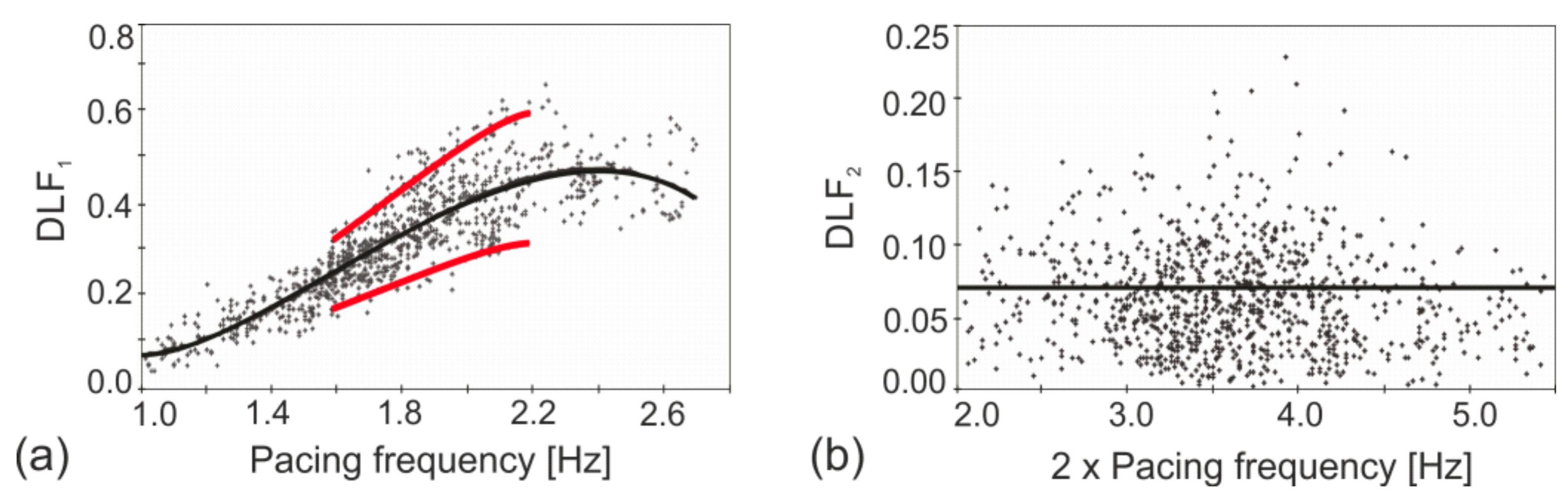
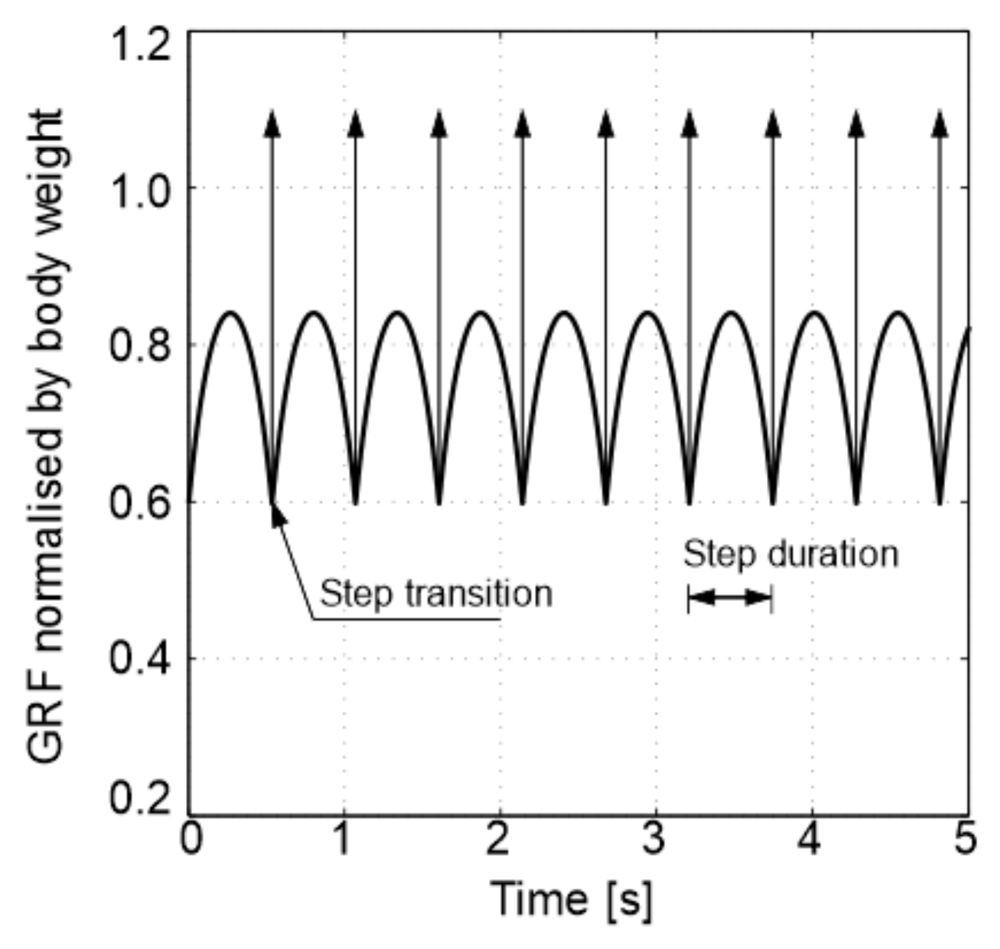
2.2. Frequency Content of Ground Reaction Force

Modelling a continuous, multi-step GRF in civil engineering applications started with summing up a sequence of nominal single-step GRFs with an appropriate time overlap between two successive steps to achieve the intended pacing frequency (and therefore time period $T$), as shown in Figure 2a [35,36]. This created a periodic force consisting of distinct harmonics in the frequency domain. The typical continuous GRF, however, is of a narrow-band nature, as shown in Figure 2b. Its energy is concentrated not only in the main harmonics that occur at the pacing frequency and its integer multiples and less pronounced sub-harmonics that are consequence of the slight differences in forces generated by the left and right foot, but it also spills over to the neighbouring frequency lines [6,37]. The main harmonics are usually normalised by the weight of the pedestrian and expressed in the form of dynamic loading factors (DLFs).

The dynamic loading factor for the first harmonic, DLF₁, shows a strong dependency on the pacing frequency (Figure 3a), while the higher harmonics are frequency independent [38] (data for the 2nd harmonic only are shown in Figure 3b). It should be noted that DLFs are independent from the pedestrian’s weight [9].

While DLF₁ can reach values as high as 0.7 (Figure 3a) for fast walking, DLF₂ (Figure 3b), DLF₃, and DLF₄ are characterised by maximum values around 0.22, 0.14, and 0.12, and mean values of 0.07, 0.06, and 0.05, respectively [38]. All four harmonics can have extremely low values approaching zero. In case of DLF₁, however, the values below 0.1 are only possible for extremely slow (and rarely seen in practice) walking frequencies below 1.3 Hz.

Figure 2. (a) Periodic GRF representation in the time domain and (b) actual GRF representation in the frequency domain (vertical component only).

Figure 2. (a) Periodic GRF representation in the time domain and (b) actual GRF representation in the frequency domain (vertical component only).

Figure 3. (a) Data points for DLF₁ versus pacing frequency. Solid black line—best data fit. Red solid lines—best fit ± 2 standard deviations. (b) Data points for DLF₂ versus pacing frequency. Solid black line—mean value. (after Kerr [38]).

Figure 3. (a) Data points for DLF₁ versus pacing frequency. Solid black line—best data fit. Red solid lines—best fit ± 2 standard deviations. (b) Data points for DLF₂ versus pacing frequency. Solid black line—mean value. (after Kerr [38]).

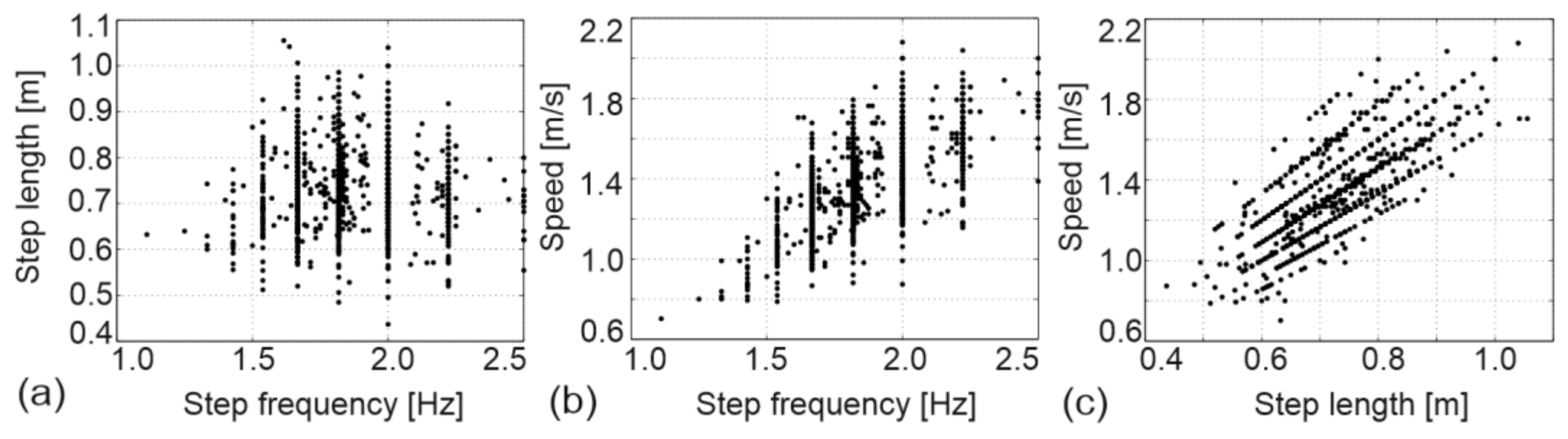
2.3. Pacing Frequency and Pedestrian’s Forward Speed

Pacing frequency is one of the most important locomotion parameters in civil engineering applications [39]. When the pacing frequency (or one of its integer multiples) is close or equal to a natural frequency of a structure that is, at the same time, light and/or lightly damped, strong vibrations that might compromise the vibration serviceability state of the structure could develop [40]. While the pacing frequency for a population of structure users is known to follow a normal distribution, the distribution parameters (the mean and the standard deviation, STD) vary between user populations and structural purpose. Table 1 shows a summary of parameters observed on nine structures. Taking the mean ± 3STD as the boundaries of the possible pacing rates in each case suggests that the pacing rate ranges from 1.3 Hz to 2.5 Hz.

Table 1. Statistics of pacing rate and walking speed on a range of structures.

Structure	Country	Sample	Pacing Rate (Hz)		Walking Speed (m/s)
[Reference]		Size	Mean	STD	Mean	STD
Road [41]	Japan	505	1.99	0.17	-	-
Footbridge 1 [42]	UK	200	1.86	0.11	1.38	0.13
Footbridge 2 [42]	UK	200	1.80	0.10	1.23	0.09
Two shopping floors [42]	UK	400	2.00	0.13	1.41	0.13
Footbridge [43]	Germany	251	1.82	0.12	1.37	0.15
Walkway [44]	Italy	116	1.84	0.17	1.41	0.22
Indoor footbridge [45]	UK	939	1.94	0.19	1.47	0.23
Footbridge [46]	Montenegro	2019	1.87	0.19	1.39	0.20

Table 1. Statistics of pacing rate and walking speed on a range of structures.

Structure	Country	Sample	Pacing Rate (Hz)		Walking Speed (m/s)
[Reference]		Size	Mean	STD	Mean	STD
Road [41]	Japan	505	1.99	0.17	-	-
Footbridge 1 [42]	UK	200	1.86	0.11	1.38	0.13
Footbridge 2 [42]	UK	200	1.80	0.10	1.23	0.09
Two shopping floors [42]	UK	400	2.00	0.13	1.41	0.13
Footbridge [43]	Germany	251	1.82	0.12	1.37	0.15
Walkway [44]	Italy	116	1.84	0.17	1.41	0.22
Indoor footbridge [45]	UK	939	1.94	0.19	1.47	0.23
Footbridge [46]	Montenegro	2019	1.87	0.19	1.39	0.20

Pedestrians’ forward speed influences the amount of time a pedestrian requires to cross a structure, and therefore, the amount of time the structure is exposed to the dynamic excitation by the pedestrian. Assuming the possible speed values are within the mean ± 3STD of the data shown in Table 1, the speed could be as low as 0.7 m/s and as high as 2.1 m/s.

Some studies also report the mean and standard deviation for the step length: 0.75 m and 0.07 m [43], 0.77 m and 0.10 m [44], and 0.74 m and 0.08 m [46]. The range of step length values can be estimated to be from 0.47 m to 1.07 m.

For any individual pedestrian, the average pedestrian speed $v$, pacing rate $f_p$, and step length $l_s$ are mutually dependent parameters ($v=f_p{l}_s$). Investigating the correlation of each pair of parameters on a population level suggests that the step length is relatively independent from the pacing frequency (Figure 4a), while the speed of walking increases with an increase in both pacing rate and step length (Figure 4b,c) [44,46].

Figure 4. (a) Step length and (b) walking speed as functions of pacing frequency. (c) Pedestrian speed as a function of step length (adapted from [46]).

Figure 4. (a) Step length and (b) walking speed as functions of pacing frequency. (c) Pedestrian speed as a function of step length (adapted from [46]).

2.4. Criteria for Evaluation of Bipedal Models

When modelling pedestrian traffic in civil engineering applications, it is important to correctly reproduce the key time- and frequency-domain features of an individual pedestrian-induced dynamic force as well as the variability in the gait parameters within the studied population. The latter aspect requires the models to be able to generate the realistic range of gait parameters (e.g., DLF, pacing rate, and walking speed) as well as to correctly represent their correlation. The ability of the two simple bipedal models (IPM and IPRFM) to reproduce kinematics and kinetics of individual walkers as well as to cover the parameter space typical of a pedestrian population is investigated in the next section.

3. Inverted Pendulum Models with Rigid Legs

The research into walking locomotion was motivated by the curiosity about its mechanics [47], and it resulted in the development of a number of bipedal models. Most of the existing models have been developed based on the observations of major determinants of walking gait: (1) pelvic rotation, (2) pelvic tilt, (3) knee flexion, (4) the foot mechanism, (5) knee mechanisms, and (6) lateral displacement of the pelvis [31]. Since this study is concerned with the investigation of the walking gait in the sagittal plane (i.e., the vertical plane that includes the direction of progression), the first and sixth determinants could be excluded from considerations.

Bipedal models of walking locomotion were initially used to study normal and pathological gaits in medical applications [31]. Apart from medicine, the walking locomotion has been a subject of interest in research fields of biomechanics, animated image processing, and robotics. A number of models are shown in Figure 5 in order of increasing complexity. A detailed representation of the first two models will be presented in this paper; we hope this will inspire a similar type of analysis for other models in the future. The main feature of all these models is that the body mass is lumped into a single point representing the BCoM. As a result, the human kinematics is represented by the movement of this single point, as dictated by the geometry (and elasticity and damping, if included) of the legs.

Figure 5. Bipedal walking locomotion models: (a) inverted pendulum [31], (b) inverted pendulum with rocker foot [30], (c) spring-loaded inverted pendulum, SLIP [48], (d) SLIP with rocker foot [49], (e) spring mass with damper [22], and (f) spring mass with rocker foot and damper [50].

Figure 5. Bipedal walking locomotion models: (a) inverted pendulum [31], (b) inverted pendulum with rocker foot [30], (c) spring-loaded inverted pendulum, SLIP [48], (d) SLIP with rocker foot [49], (e) spring mass with damper [22], and (f) spring mass with rocker foot and damper [50].

3.1. Inverted Pendulum Model

The inverted pendulum model (IPM) is the simplest bipedal walking model (Figure 5a) developed by Saunders et al. [31]. The model consists of a point mass $m_p$ and two rigid, straight, and massless legs (Figure 6). The human body is assumed to be symmetrical, i.e., the two legs have the same length. The foot is modelled as a point foot that does not slip during contact with the ground.

The time instant when one leg touches the ground can be taken as a starting point of a step in the IPM. The model is set into motion by specifying the initial conditions for the attack angle ${\theta }_0$ and angular speed ${\dot{\theta }}_0$. The resulting motion of the point mass is in the form of an arc, defined by the geometry of the supporting leg. A step is completed when the angle formed by the supporting leg, $\theta \left(t\right)$, (see Figure 6) becomes equal to the supplement of the attack angle ${\theta }_0$. This angle is also called the end-of-step angle, denoted as ${\theta }_e$ in Figure 6.

At the time of step completion, the swinging leg touches the ground and the pedestrian’s weight is instantaneously transferred from one foot to another. The next step is initiated by specifying a new set of initial conditions, which are usually assumed to be the same for all the steps.

Using the Lagrangian approach [51], the equation of motion for a single step can be written as:

$$\ddot{\theta }\left(t\right)=\frac{\cos \theta \left(t\right)}{l}g,$$

(1)

where $\ddot{\theta }\left(t\right)$ is the second derivative of $\theta \left(t\right)$ with respect to time, $l$ is the distance from the BCoM to the foot (hereafter referred to as the pendulum length), and $g$ is the acceleration of gravity ($g=-9.81$ m/s²). Equation (1) describes the stance phase of the gait cycle only because the IPM neglects the DSP. The GRF generated within a single step $F_p\left(t\right)$ is:

$$F_p\left(t\right)=-m_p\sin \theta \left(t\right)\left(g\sin \theta \left(t\right)+l\dot{\theta }{\left(t\right)}^2\right),$$

(2)

where $\dot{\theta }\left(t\right)$ is the first derivative of $\theta \left(t\right)$ with respect to time, while all other variables are the same as before.

The step transition process requires redirecting the BCoM upwards, from the falling downwards momentum at the end of a step. During walking, this upwards momentum is provided by a foot pushing off the ground just before the toe-off event (Figure 1), and it can be simulated in the model by applying an upward impulse to the point mass. The amplitude of this vertical upward impulse $I_n$ at the end of the nth step is [16]:

$$I_n=-m_p{\dot{y}}_{e,n}+m_p{\dot{x}}_{0,n+1}{\cot \dot{\theta }}_0,$$

(3)

where ${\dot{y}}_{e,n}$ and ${\dot{x}}_{0,n+1}$ are the vertical speed of the BCoM at the end of the nth step and the forward speed at the beginning of the (n + 1)th step, respectively. The first part of the impulse in Equation (3) cancels the falling effect at the end of nth step, while the second part pushes the mass upwards so to supply the initial forward speed ${\dot{x}}_{0,n+1}$. The initial forward speed ${\dot{x}}_0$ is assumed to be the same in all steps and it is linked to the initial angular speed ${\dot{\theta }}_0$ and the attack angle ${\theta }_0$ through the equation:

$${\dot{x}}_0=l{\dot{\theta }}_0{\sin \theta }_0.$$

(4)

3.1.1. Model Inputs

To perform simulations using the IPM, two sets of input parameters are required: model parameters and initial conditions. The model parameters consist of pedestrian mass and the pendulum length. The body mass of 77.5 ± 17.2 kg (mean ± STD) and height of 1.676 ± 0.097 m of an average person are chosen as representative values in this paper [52]. This body height corresponds to the physical leg length of 0.864 ± 0.050 m [53]. The physical leg length has to be increased by about 20% [54] to obtain the pendulum length parameter, which amounts to 1.037 ± 0.060 m.

Initial conditions required by the model are ${\theta }_0$ and ${\dot{\theta }}_0$ (or ${\dot{x}}_0$ instead of ${\dot{\theta }}_0$, see Equation (4)). The attack angle ${\theta }_0$ ranges between 65° and 80° [48]. The exact range of the initial forward speed ${\dot{x}}_0$ is not well known. After initial simulation trials, the range has been set to 1.0–2.5 m/s for the needs of the parametric study. The locomotion is assumed to be periodic, i.e., the initial conditions remain constant in each step.

3.1.2. Simulation Results

The solver ode45 from the MATLAB library [55] that utilises the Runge–Kutta integration method with a variable step size was used to solve Equation (1). The maximum time step of the solver is set at 10⁻³ s. An example of the GRF generated by the model for the input values of $m_p=$ 77.5 kg, $l=$ 1.037 m, ${\theta }_0=$ 69°, and ${\dot{x}}_0=$ 1.61 m/s is shown in Figure 7. The initial conditions were chosen to generate walking at a pacing rate of 1.87 Hz and an average walking speed of 1.39 m/s, which correspond to the mean values observed on an as-built bridge (reported in [46], and included in Table 1). The arcs in the figure represent the inertia force of mass $m_p$ while the vertical lines represent the externally applied impulses. The duration of each impulse for the numerical simulation is chosen to be such that the average of the total force is equal to the pedestrian weight.

The amplitude of the first harmonic of this GRF is within the measured range shown in Figure 3. The DLFs for higher harmonics in the IPM are significantly overestimated due to the simplified modelling of the push-off phase using the impulses [17].

To investigate the ability of the IPM to reproduce realistic combinations of the pacing rate, DLF₁, step length, and average forward speed, the model has been exposed to a range of initial conditions: the initial forward speed varies between 1.0 m/s and 2.5 m/s (in discrete steps of 0.01 m/s) and the attack angle varies between 65° and 80° (in steps of 0.01°). The light grey area in Figure 8a shows all the combinations of the attack angle and initial forward speed that result in the physically relevant pacing rate between 1.3 and 2.5 Hz. The light grey in Figure 8b covers the parameter space which results in DLF₁ ≤ 0.7, while the darker grey in the same figure represents the parameter combinations that produce realistic values of both the pacing frequency and DLF₁. It can be seen that unrealistically low values of DLF₁ (i.e., DLF₁ ≤ 0.1) correspond to an unrealistically low pacing frequency, which is consistent with the data shown in Figure 3a. The light grey area in Figure 8c shows a parameter space that covers the realistic range of the walking speed (0.7–2.1 m/s) and the dark grey area in the same figure represents all the parameter combinations that result in a realistic pacing frequency, DLF₁, and pedestrian speed. Figure 8c reveals that, for the given pendulum parameters (i.e., $m_p=$ 77.5 kg, $l=$ 1.037 m), the most extreme pedestrian speeds (i.e., around 0.7 m/s and 2.1 m/s) are not achievable. To better represent extremely slow walkers, the pendulum length must be shortened, while the fastest walkers can be modelled by lengthening the pendulum length. Using a pendulum length between 0.9 m and 1.2 m (in agreement with the data reported by Hof et al. [54], it is possible to select initial conditions that result in realistic simulations of all of the pacing frequencies, DLF₁, and walking speeds.

To check the correlation between the gait parameters of interest, only those initial conditions that produced realistic ranges of the pacing rate, DLF₁, and average forward speed are utilised in Figure 9. The boundary of the parameter space that includes the points within the dark grey area in Figure 8c are shown as solid lines in Figure 9. Boundaries are also shown for a shorter pendulum length of 0.9 m (dashed line) and elongated pendulum length of 1.2 m (chain line). In addition, the experimental data points from Figure 4 are also shown in Figure 9a–c, while the boundaries for DLF₁ from Figure 3a are shown in Figure 9d. Figure 9 shows that the IPM is able to reproduce a (empirically observed) lack of correlation between the step length and the step frequency, as well as the positive correlations between the speed and step frequency, speed and step length, and DLF₁ and step frequency. It is also noticeable that the model covers a larger parameter space than that seen in practice (e.g., for a given step frequency of, say, 2 Hz, it can both underestimate and overestimate the DLF₁ value, depending on the choice of the pendulum length and the initial conditions).

The trajectory of the BCoM that is represented by a series of arcs in the IPM overestimates the vertical excursion by a factor of two or more [56]. The trajectory also lacks smoothness of the actual trajectory shown in Figure 1 due to an instantaneous transfer of the body weight from one foot to another and the inherent inability of the IPM to depict the double support phase of the gait.

The inability of the IPM to replicate the kinematics of the BCoM accurately is a drawback for the quantitative modelling of pedestrians on a vibrating structure as the kinematic state of the foot–structure interface cannot be genuinely represented. On the other hand, this simple model is a building block for understating more complex bipedal models and could offer some qualitative insight into the pedestrian–structure interaction [16,17].

Figure 8. (a) Pacing rate, (b) DLF₁, and (c) average forward speed of a pedestrian resulting from different combinations of the initial conditions in the IPM ($m_p=$ 77.5 kg, $l=$ 1.037 m). Refer to the text for explanation of the colours.

Figure 8. (a) Pacing rate, (b) DLF₁, and (c) average forward speed of a pedestrian resulting from different combinations of the initial conditions in the IPM ($m_p=$ 77.5 kg, $l=$ 1.037 m). Refer to the text for explanation of the colours.

Figure 9. Relationships between (a) step length and step frequency, (b) speed and step frequency, (c) speed and step length, and (d) DLF₁ and step frequency, in the IPM. Blue dashed line: $l=$ 0.9 m, black solid line: $l=$ 1.037 m, red chain line: $l=$ 1.2 m. Black dots: experimental data from Figure 4. Dotted lines: experimental data (mean and mean ± 2 STD) by Kerr [38].

Figure 9. Relationships between (a) step length and step frequency, (b) speed and step frequency, (c) speed and step length, and (d) DLF₁ and step frequency, in the IPM. Blue dashed line: $l=$ 0.9 m, black solid line: $l=$ 1.037 m, red chain line: $l=$ 1.2 m. Black dots: experimental data from Figure 4. Dotted lines: experimental data (mean and mean ± 2 STD) by Kerr [38].

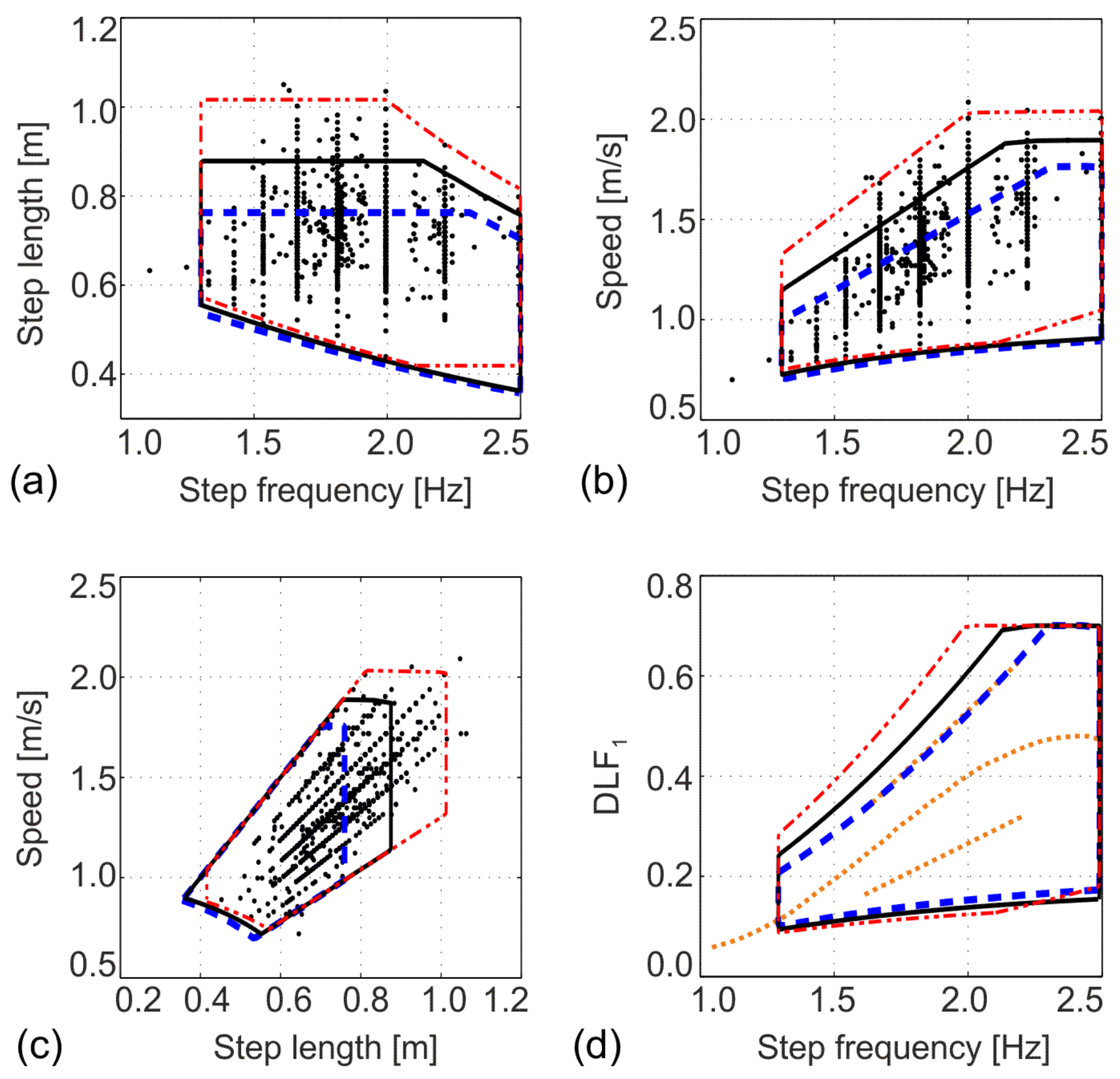
3.1.3. Dimensional Analysis

Dimensional analysis is a convenient means of exploring how changing some parameters influences the others. Let us select mass $m_p$, pendulum length $l$, and acceleration of gravity $g$ as the base quantities. For a given attack angle ${\theta }_0$, it is possible to determine how changing the $m_p$ or $l$ (or gravity $g$, although this change is not of actual interest in this work) influences other parameters of interest. The new value of a parameter of interest can be found by preserving the dimensionless value, defined in

Table 2. Parameters of interest.

Parameter	Dimensionless Parameter
Step frequency $f_p$	$f_p^{\ast }=f_p\sqrt{\frac{l}{g}}$
Step length $d$	$d^{\ast }=\frac{d}{l}$
Average speed $v$	$v^{\ast }=\frac{v}{\sqrt{gl}}$
Dynamic load factor DLF1	-

, for the same parameter.

This can be used, for example, to observe consequences of extending the pendulum length from, say, 1.037 m to 1.2 m. Let us assume the initial conditions: ${\theta }_0=70°$ and ${\dot{x}}_0=$ 1.5 m/s. These inputs (for $l=$ 1.037 m) correspond to the following gait parameters: $f_p=$ 1.79 Hz and $v=$ 1.27 m/s (Figure 8). In addition, DLF₁ = 0.31. Extending the pendulum length to 1.2 m, keeping the same attack angle, and using dimensional analysis leads to an increase in the initial forward speed from ${\dot{x}}_0=$ 1.5 m/s to ${\dot{x}}_0\sqrt{1.2/1.037}=$ 1.61 m/s. Table 2 indicates that the step frequency would reduce to $1.79\sqrt{1.037/1.2}=$ 1.66 Hz, the average speed of walking would increase to 1.27$\sqrt{1.2/1.037}=$ 1.36 m/s, while DLF₁, being a dimensionless quantity, would remain 0.31. Moreover, the step length can now be calculated as a ratio between the average speed and step frequency. It has increased from 0.71 m (1.27 m/s/1.79 Hz) to 0.82 m (1.36 m/s/1.66 Hz), which corresponds to the expected increase by a multiplication factor of 1.2/1.037 (Table 2). A change in the pedestrian mass, on the other hand, does not influence the resulting parameters. However, an increase in the pedestrian mass will proportionally increase the harmonic force value, given that DLF₁ represents the force normalised by a pedestrian’s weight.

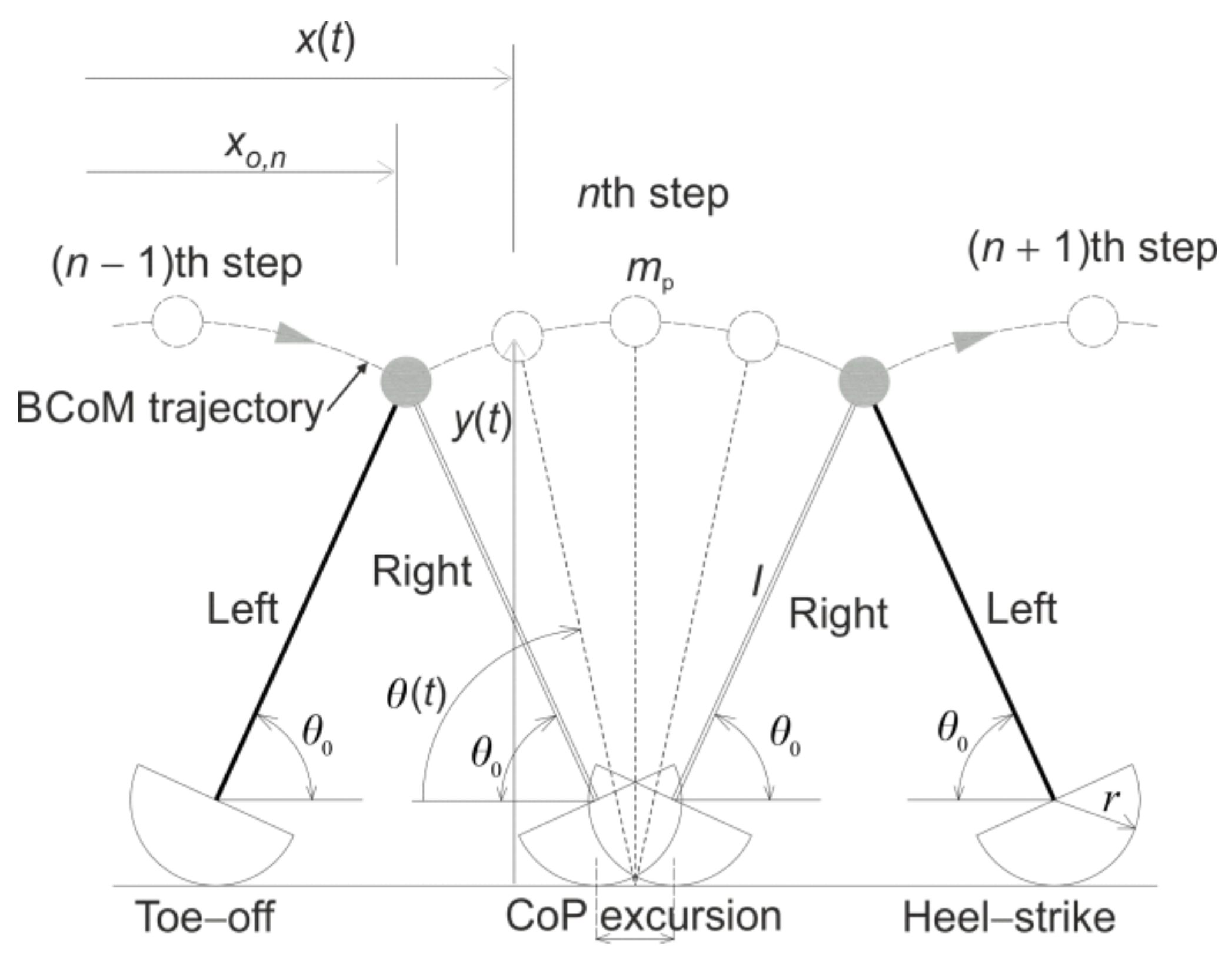
3.2. Inverted Pendulum with Rocker Foot Model

The IPM overestimates the vertical excursion of the BCoM since it does not include all the relevant determinants of the walking gait in the modelling process [31]. While pelvic tilt and knee flexion (the second and third determinants) have little or no effect on the amount of the vertical excursion [57,58], the foot and ankle mechanisms (the fourth and fifth determinants) influence the excursion significantly. Thus, a way to improve the modelling of the vertical excursion is to replace point foot with a rocker. This intervention results in the inverted pendulum with the rocker foot model, IPRFM, shown in Figure 10 and explained in more detail by Hansen et al. [59], and Gard and Childress [30].

The introduction of the rocker, in the form of a circular arc having radius $r$, is equivalent to lengthening the pendulum length of the IPM. In addition, it represents the walking mechanism during the stance phase more accurately as it enables the transition of the centre of pressure (CoP) from the “heel” to the “toe” as the foot rolls forward. Although the trajectory of the BCoM in the IPRFM still follows the pattern of a series of arcs, the effective lengthening of the leg and the forward progression of the CoP reduce the total excursion of the BCoM in comparison with the IPM [56,59].

Using the Lagrangian approach, the equation of motion for the IPRFM can be written as:

$$\ddot{\theta }\left(t\right)=\frac{l \cos \theta \left(t\right) \left(g-r{\dot{\theta }}^2\left(t\right)\right)}{r^2+l^2+2rl\sin \theta \left(t\right)}.$$

(5)

The GRF generated by the IPRFM within a single step is:

$$F_p\left(t\right)=-m_p\left(g+l{\dot{\theta }}^2\left(t\right)\sin \theta \left(t\right)-\frac{l^2{\cos }^2\theta \left(t\right) (g-r{\dot{\theta }}^2\left(t\right))}{r^2+l^2+2rl\sin \theta \left(t\right)}\right).$$

(6)

The end-of-the-step condition and the amplitude of applied impulses are calculated using the same approach as in the calculations for the IPM.

3.2.1. Model Inputs

The inputs for the IPRFM are pendulum length, $l+r,$ and body mass, $m_p$. They are chosen in the same way as for the IPM. In addition, the proportion of $r$ in the pendulum length has to be specified. McGeer [47] assumed that the supporting foot travels a distance of 20% of the leg length, and calculated that this requires a roller radius $r$ that is equal to 30% of the leg length. Whittington and Thelen [49] reported that a roller radius of 0.3 m, which is approximately 30% of the limb length, resulted in the centre of pressure excursion that best agreed with experimental data at slow, preferred, and fast walking speeds. Adamczyk et al. [60] added that this size of the rolling feet appeared energetically advantageous, partially due to decreased work in step-to-step transitions. Hence, the rocker radius of 0.3 m is adopted in this paper.

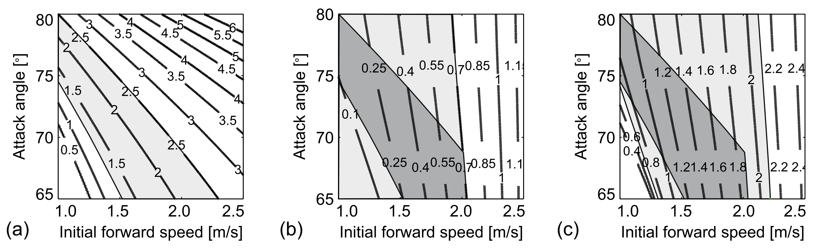
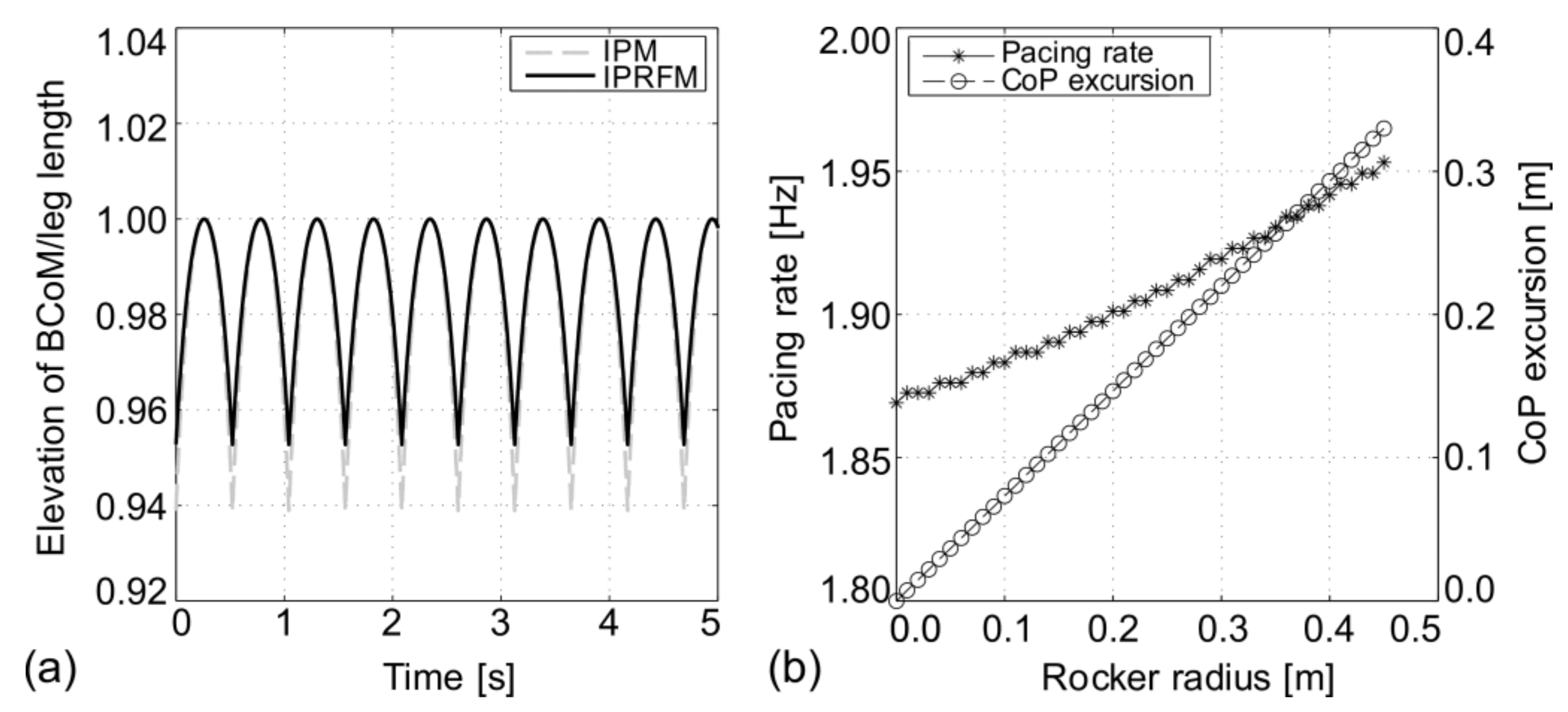
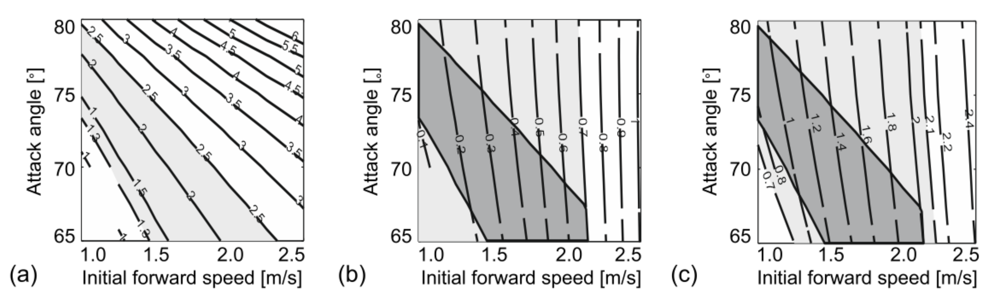
3.2.2. Simulation Results

As before, ode45 solver utilising the Runge–Kutta integration with a variable step size was implemented to solve the differential equation. Figure 11a shows how the introduction of a rocker in the IPRFM reduces the vertical excursion of the BCoM when compared with the IPM, while Figure 11b demonstrates that the progression of the CoP (i.e., excursion of the CoP in Figure 10) and the pacing frequency both increase with an increase in the rocker radius from 0.00 m to 0.45 m.

The results of a parametric scan of the IPRFM are shown in Figure 12. The rocker radius was set to $r=$ 0.3 m and length $l+r=$ 1.037 m. As before, the initial forward speed ranges from 1.0 m/s to 2.5 m/s, and the attack angle is between 65° and 80°. The light grey area in Figure 12a shows all the combinations of the initial conditions that result in the expected pacing rate between 1.3 and 2.5 Hz. Among the identified combinations, those that also result in a viable value of DLF₁ ≤ 0.7 are shown as the dark grey area in Figure 12b. Furthermore, the dark grey area in Figure 12c denotes the parameter space that results in viable values of the pacing rate, DLF₁, and the average forward speed. In comparison with the IPM (Figure 8c), the IPRFM provides a slightly wider range of initial conditions that result in realistic walking parameters (Figure 12c). Varying the leg length and/or the rocker radius offers further flexibility in modelling different pedestrians.

Figure 13 shows that the correlation graphs typical of the IPRFM are similar to those derived for the IPM in Figure 9. The solid lines represent the $l+r=$ 1.037 m case, whereby $l=$ 0.737 m and $r=$ 0.3 m. The chain lines are derived for $l+r=$ 1.2 m (achieved by increasing the original value for either $l$ or $r$) and the dashed lines are for $l+r=$ 0.9 m (achieved by decreasing either $l$ or $r$). As before, increasing the pendulum length enables the modelling of pedestrians with the longest step lengths and fastest walking speeds, while a decrease in the pendulum length has the opposite effect. However, the pendulum length increase also increases the DLF₁ to values not easily encountered in practice. The lower boundary for DLFs underestimates the measured values for almost all but the slowest pacing frequencies. There is little difference between the cases having the same value of $l+r$ in Figure 13a–c, suggesting similar effects on the parameter space are achieved by changing either $l$ or $r$. The effects on the DLF parameter are slightly more noticeable.

In summary, the IPRFM is a kinematic upgrade of the IPM as it reduces the vertical excursion of the BCoM and enables the progression of the CoP. However, it still models the single support phase of the gait only and requires applying the impulses as an external source of power to keep the model in motion. The latter means that the generated GRF has the same shortcomings as the IPM in terms of overestimating the higher harmonics.

Figure 13. Relationships between (a) step length and step frequency, (b) speed and step frequency, (c) speed and step length, and (d) DLF1 and step frequency, in the IPRFM. Blue dashed lines: $l+r=$ 0.9 m (thick $l=$ 0.6 m and $r=$ 0.3 m, thin $l=$ 0.737 m and $r=$ 0.163 m), black solid line: $l+r=$ 1.037 m (thick $l=$ 0.737 m and $r=$ 0.3 m), red chain lines: $l+r=$ 1.2 m (thick $l=$ 0.9 m and $r=$ 0.3 m, thin $l=$ 0.737 m and $r=$ 0.463 m). Black dots: experimental data from Figure 4, yellow thin solid lines in (d): experimental data (mean ± 2 STD) by Kerr [38].

Figure 13. Relationships between (a) step length and step frequency, (b) speed and step frequency, (c) speed and step length, and (d) DLF1 and step frequency, in the IPRFM. Blue dashed lines: $l+r=$ 0.9 m (thick $l=$ 0.6 m and $r=$ 0.3 m, thin $l=$ 0.737 m and $r=$ 0.163 m), black solid line: $l+r=$ 1.037 m (thick $l=$ 0.737 m and $r=$ 0.3 m), red chain lines: $l+r=$ 1.2 m (thick $l=$ 0.9 m and $r=$ 0.3 m, thin $l=$ 0.737 m and $r=$ 0.463 m). Black dots: experimental data from Figure 4, yellow thin solid lines in (d): experimental data (mean ± 2 STD) by Kerr [38].

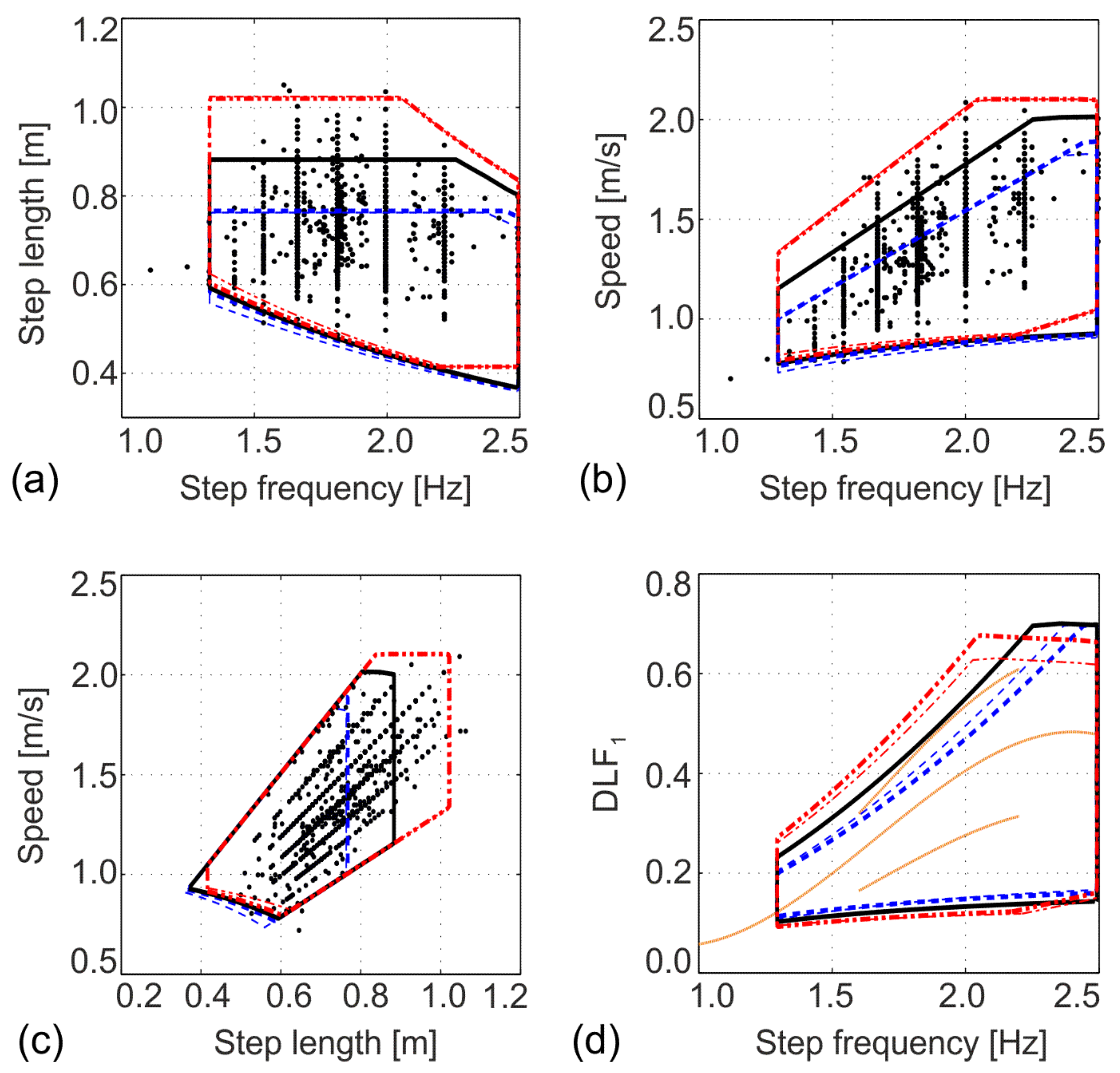
3.2.3. Dimensional Analysis

As in the case of the IPM, the three base quantities ($m_p$, $l$ and $g$) are used to determine how changing $m_p$ or $l$ influences other parameters of interest for a given ${\theta }_0$. Both $r$ and $l$ have a dimension of length, and therefore, multiplying $l$ by the factor $l^{\ast }$ would require multiplying $r$ by the same factor. The dimensionless parameters of interest are the same as those presented in Table 2.

Let us assume the initial conditions: ${\theta }_0={70}^{°}$ and ${\dot{x}}_0=$ 1.5 m/s. These inputs correspond to $f_p=$ 1.85 Hz and $v=$ 1.32 m/s (Figure 12). In addition, DLF₁ = 0.30. Let us observe how extending length $l+r=1.037$ m (whereby $l=0.737$ m and $r=0.3$ m) to $l^{\ast }\left(l+r\right)=$ 1.2 m influences the other derived parameters. This corresponds to $l^{\ast }=1.2/1.037=1.16$, and therefore, the new lengths $l=0.853$ m and $r=0.347$ m. Dimensional analysis (Table 2) suggests that the observed lengthening of the pendulum results in the initial forward speed, which increases from ${\dot{x}}_0$= 1.5 m/s to ${\dot{x}}_0\sqrt{1.16}=$ 1.61 m/s. The step frequency will reduce to ${\dot{x}}_0\sqrt{1/1.16}=$ 1.72 Hz, the average speed of walking will increase to $1.32\sqrt{1.16}=$ 1.42 m/s, while DLF₁ will remain 0.30. The step length (a ratio between the average speed and step frequency) has increased from 0.71 m (1.32 m/s/1.85 Hz) to 0.82 m (1.42 m/s/1.72 Hz), which corresponds to the expected increase by a multiplication factor of 1.16 (Table 2). The change in the pedestrian mass does not influence any quantity apart from the harmonic force amplitude.

4. Discussion and Conclusions

Both the IPM and IPRFM are simplifications of human gait that have no capability of modelling the double support phase of walking locomotion. As a result, the kinematics of the body’s centre of mass consists of a series of arcs with a non-smooth transition between the successive steps. The vertical excursion of the centre of mass is exaggerated in the IPM and reduced to a more realistic level by enabling the forward progression of the centre of pressure in the IPRFM. However, due to a lack of the double support phase, the kinematics in the two models are unrepresentative of actual human walking. As the kinematic compatibility of the leg and vibrating surface is likely to play an important role in the realistic simulation of actual walking on lively structures, it is unrealistic to expect that these models can be used in a quantitative vibration serviceability assessment of civil engineering structures. Initial research into using the IPM on lively structures confirms this notion. Namely, simulations by Bocian et al. [16] demonstrated that the IPM produces reasonable estimates of additional damping that pedestrians could add to the structures under a specific vibration frequency, pacing frequency, and vibration amplitude conditions, as observed in practice. However, the IPM also predicts negative damping effects for some parameter combinations—a phenomenon that has not been observed in practice so far. In addition, Dang [17] demonstrated that the IPM, on average, generates an improved prediction of the measured vibration response compared with the classical harmonic force model that neglects the pedestrian–structure interaction. At the same time, however, the IPM tends to react to the oscillating structure by reducing the pacing rate, especially when the pacing rate is close to the natural frequency of the structure. This is in contradiction with the slight increase in the pacing rate observed in experiments, and it makes the model erroneous in the most important frequency region. The authors are unaware of the research that investigated the performance of the IPRFM on lively structures.

Parametric analysis focused on the gait parameters for the two models showed that they are able to generate realistic combinations of the gait parameters and their correlations. In addition, they include some parameter combinations that are not seen in pedestrian populations. Namely, a realistic value for one parameter, say DLF₁, is not necessarily associated with the realistic values of the other parameters, e.g., pacing frequency. The introduction of the rocker foot has a kinematic effect similar to extending the pendulum length in the IPM. However, the ranges of the locomotion parameters that the two models can produce are similar, with no obvious advantage of using one model over another. Finally, it should be noticed that the two models have the ability to generate a realistic value of the DLF₁, while higher harmonics are overestimated due to presence of impulse components in the dynamic force.

The next natural step in the evolution of pedestrian modelling is to replace the rigid leg with a compliant (i.e., deformable) leg (with or without a rocker foot), which is a feature of the spring-loaded inverted pendulum, SLIP, models (Figure 5c,d). These models are known to improve the kinematics of the body centre of mass and replicate a typical M-shaped GRF pattern [48]. However, these models, together with the two models analysed in this paper, neglect the role of the muscles in generating walking locomotion by relying on either artificially generated external impulses (as in the IPM and IPRFM) or energy preservation (in SLIP models). They also neglect the energy dissipation that characterises the walking process [32]. In response to these drawbacks, models that account for leg damping and positive work done by muscles have been developed (Figure 5e,f). Both constant [50] and time-variant damping models [22,23,61] exist. They propose different modelling mechanisms for compensating the energy lost due to damping. This brief model overview illustrates the richness of modelling approaches within the inverted pendulum model family. Unfortunately, the verification of these models, especially on lively structures, lags behind the theoretical developments. The adoption of one or more models in the vibration serviceability field could be accelerated by: (1) the development of an open-access database of experimental data related to walking on lively structures (that preferably should include kinematic and kinetic data for the human, as well as vibration data for the structure) and (2) providing detailed insight into the performance of the inverted pendulum models on both rigid and lively surfaces.

To conclude, the IPM and IPRFM are the simplest models from the bipedal family of models of pedestrians. This paper provides the necessary background for the application of these models by other researchers and information about their ability to represent kinematic and kinetic features that characterise human walking locomotion on rigid level surfaces. A limited amount of research into the performance of the IPM on lively structures suggests that, while the model can qualitatively describe some effects observed on as-built structures, it cannot be relied upon for the accurate assessment of structural vibration, especially in the most interesting case of (near) resonance excitation. Further research should investigate whether more complex bipedal models could provide a better representation of pedestrian locomotion on both rigid and lively surfaces.

References

1. BS 5400; Steel, Concrete and Composite Bridges-Part 2: Specification for Loads; Appendix C: Vibration Serviceability Requirements for Foot and Cycle Track Bridges. British Standards Association: London, UK, 1978.
2. Sétra. Footbridges: Assessment of Vibrational Behaviour of Footbridges under Pedestrian Loading: Technical Guide; Service d’Études Techniques des Routes et Autoroutes: Paris, France, 2006. [Google Scholar]
3. NA to BS EN 1991-2:2003; UK National Annex to Eurocode 1: Actions on Structures-Part 2: Traffic Loads on Bridges. British Standards Institution: London, UK, 2008.
4. Research Fund for Coal and Steel. Human Induced Vibrations of Steel Structures: Design of Footbridges—Guideline. RFS2-CT-2007-00033. 2009. Available online: https://www.coursehero.com/file/59133890/Footbridge-Backgroundpdf/ (accessed on 5 April 2013).
5. Brownjohn, J.M.W.; Pavic, A.; Omenzetter, P. A spectral density approach for modelling continuous vertical forces on pedestrian structures due to walking. Can. J. Civ. Eng. 2004, 31, 65–77. [Google Scholar] [CrossRef]
6. Živanović, S.; Pavic, A.; Reynolds, P. Probability based prediction of multi-mode vibration response to walking excitation. Eng. Struct. 2007, 29, 942–954. [Google Scholar] [CrossRef]
7. Caprani, C.C.; Keogh, J.; Archbold, P.; Fanning, P. Enhancement factors for the vertical response of footbridges subjected to stochastic crowd loading. Comput. Struct. 2012, 102–103, 87–96. [Google Scholar] [CrossRef]
8. Piccardo, G.; Tubino, F. Equivalent spectral model and maximum dynamic response for the serviceability analysis of footbridges. Eng. Struct. 2012, 40, 445–456. [Google Scholar] [CrossRef]
9. Racic, V.; Brownjohn, J.M.W. Stochastic model of near periodic vertical loads due to humans walking. Adv. Eng. Inform. 2011, 25, 259–275. [Google Scholar] [CrossRef]
10. Dallard, P.; Fitzpatrick, A.J.; Flint, A.; Le Bourva, S.; Low, A.; Ridsdill-Smith, R.M.; Willford, M. The London Millennium Footbridge. Struct. Eng. 2001, 79, 17–33. [Google Scholar]
11. Macdonald, J.H.G. Lateral excitation of bridges by balancing pedestrians. Proc. R. Soc. Lond. Ser. A 2009, 465, 1055–1073. [Google Scholar] [CrossRef]
12. Ingólfsson, E.T.; Georgakis, C.T.; Ricciardelli, F.; Jönsson, J. Experimental identification of pedestrian-induced lateral forces on footbridges. J. Sound Vib. 2011, 330, 1265–1284. [Google Scholar] [CrossRef]
13. Carroll, S.P.; Owen, J.S.; Hussein, M.F.M. Experimental identification of the lateral human-structure interaction mechanism and assessment of the inverted-pendulum biomechanical model. J. Sound Vib. 2014, 333, 5865–5884. [Google Scholar] [CrossRef]
14. McRobie, A.; Morghental, G.; Lasenby, J.; Ringer, M. Section model tests on human-structure lock-in. Proc. ICE-Bridge Eng. 2003, 156, 71–79. [Google Scholar] [CrossRef]
15. Ricciardelli, F.; Mafrici MIngólfsson, E.T. Lateral Pedestrian-Induced Vibrations of Footbridges: Characteristics of Walking Forces. J. Bridge Eng. 2014, 19, 04014035. [Google Scholar] [CrossRef]
16. Bocian, M.; Macdonald, J.H.G.; Burn, J.F. Biomechanically-inspired modelling of pedestrian-induced vertical self-excited forces. J. Bridge Eng. 2013, 18, 1336–1346. [Google Scholar] [CrossRef]
17. Dang, H.V. Experimental and Numerical Modelling of Walking Locomotion on Vertically Vibrating Low-Frequency Structures. Ph.D. Thesis, University of Warwick, Coventry, UK, 2014. [Google Scholar]
18. Ahmadi, E.; Caprani, C.; Živanović, S.; Heidarpour, A. Vertical ground reaction forces on rigid and vibrating surfaces for vibration serviceability assessment of structures. Eng. Struct. 2018, 172, 723–738. [Google Scholar] [CrossRef]
19. Ahmadi, E.; Caprani, C.; Živanović, S.; Heidarpour, A. Assessment of human-structure interaction on a lively lightweight GFRP footbridge. Eng. Struct. 2019, 199, 109687. [Google Scholar] [CrossRef]
20. Caprani, C.C.; Ahmadi, E. Formulation of human-structure interaction system models for vertical vibration. J. Sound Vib. 2016, 377, 346–367. [Google Scholar] [CrossRef]
21. Bocian, M.; Macdonald, J.H.G.; Burn, J.F. Biomechanically inspired modelling of pedestrian-induced forces on laterally oscillating structures. J. Sound Vib. 2012, 331, 3914–3929. [Google Scholar] [CrossRef]
22. Qin, J.W.; Law, S.S.; Yang, Q.S.; Yang, N. Pedestrian-bridge dynamic interaction, including human participation. J. Sound Vib. 2013, 332, 1107–1124. [Google Scholar] [CrossRef]
23. Lin, B.; Zhang, Q.; Fan, F.; Shen, S. A damped bipedal inverted pendulum for human-structure interaction analysis. Appl. Math. Model. 2020, 87, 606–624. [Google Scholar] [CrossRef]
24. Vega Ruiz, D.; Magluta, C.; Roitman, N. Experimental verification of biomechanical model of bipedal walking to simulate vertical loads induced by humans. Mech. Syst. Signal Process. 2022, 167, 108513. [Google Scholar] [CrossRef]
25. Carroll, S.P.; Owen, J.S.; Hussein, M.F.M. Modelling crowd-bridge dynamic interaction with a discretely defined crowd. J. Sound Vib. 2012, 331, 2685–2709. [Google Scholar] [CrossRef]
26. Whittle, M.W. Gait Analysis: An Introduction, 3rd ed.; Butterworth-Heinemann Elsevier: Oxford, UK, 2001. [Google Scholar]
27. Inman, V.T.; Ralston, H.; Todd, F. Human Walking; Edwin Mellen Press Ltd.: Lewiston, NY, USA, 1989. [Google Scholar]
28. Perry, J.; Burnfield, J.M. Gait Analysis: Normal and Pathological Function, 2nd ed.; SLACK Incorporated: Thorofare, NI, USA, 2010. [Google Scholar]
29. Ayyappa, E. Normal human locomotion, Part 2: Motion, ground-reaction force and muscle activity. Prosthet. Orthot. 1997, 9, 4957. [Google Scholar] [CrossRef]
30. Gard, S.A.; Childress, D.S. What determines the vertical displacement of the body during normal walking? J. Prosthet. Orthot. 2001, 13, 6467. [Google Scholar] [CrossRef]
31. Saunders, J.B.D.M.; Inman, V.T.; Eberhart, H.D. The major determinants in normal and pathological gait. J. Bone Jt. Surg. 1953, 53, 543–558. [Google Scholar] [CrossRef]
32. Cavagna, G.A.; Thys, H.; Zamboni, A. The sources of external work in level walking and running. J. Physiol. 1976, 262, 639657. [Google Scholar] [CrossRef]
33. Whittle, M.W. Three-dimensional motion of the center of gravity of the body during walking. Hum. Mov. Sci. 1997, 16, 347–355. [Google Scholar] [CrossRef]
34. Gard, S.A.; Miff, S.C.; Kuo, A.D. Comparison of kinematic and kinetic methods for computing the vertical motion of the body center of mass during walking. Hum. Mov. Sci. 2004, 22, 597610. [Google Scholar] [CrossRef]
35. Blanchard, J.; Davies, B.L.; Smith, J.W. Design criteria and analysis for dynamic loading of footbridges. In Proceedings of the Symposium on Dynamic Behaviour of Bridges at the Transport and Road Research Laboratory, Crowthorne, UK, 19 May 1977; pp. 90–100. [Google Scholar]
36. Rainer, J.H.; Pernica, G. Vertical dynamic forces from footsteps. Can. Acoust. 1986, 14, 12–21. [Google Scholar]
37. Racic, V.; Pavic, A.; Brownjohn, J.M.W. Experimental identification and analytical modelling of human walking forces: Literature review. J. Sound Vib. 2009, 326, 1–49. [Google Scholar] [CrossRef]
38. Kerr, S.C. Human Induced Loading on Staircases. Ph.D. Thesis, University College London, London, UK, 1998. [Google Scholar]
39. Pedersen, L.; Frier, C. Sensitivity of footbridge vibrations to stochastic walking parameters. J. Sound Vib. 2010, 29, 2683–2701. [Google Scholar] [CrossRef]
40. Živanović, S.; Pavic, A.; Reynolds, P. Vibration serviceability of footbridges under human-induced excitation: A literature review. J. Sound Vib. 2005, 279, 1–74. [Google Scholar] [CrossRef]
41. Matsumoto, Y.; Nishioka, T.; Shiojiri, H.; Matsuzaki, K. Dynamic design of footbridges. IABSE Proc. 1978, P-17/78, 1–15. [Google Scholar]
42. Pachi, A.; Ji, T. Frequency and velocity of people walking. Struct. Eng. 2005, 83, 36–40. [Google Scholar]
43. Kasperski, K.; Sahnaci, C. Serviceability of Pedestrian Structures. In Proceedings of the IMAC-XXV, Orlando, FL, USA, 19–22 February 2007. [Google Scholar]
44. Ricciardelli, F.; Briatico, C.; Ingólfsson, E.T.; Georgakis, C.T. Experimental validation and calibration of pedestrian loading models for footbridges. In Proceedings of the International Conference of Experimental Vibration Analysis for Civil Engineering Structures, Porto, Portugal, 24–26 October 2007. [Google Scholar]
45. Živanović, S.; Racic, V.; El-Bahnasy, I.; Pavic, A. Statistical characterization of parameters defining human walking as observed on an indoor passerelle. In Proceedings of the International Conference of Experimental Vibration Analysis for Civil Engineering Structures, Porto, Portugal, 24–26 October 2007. [Google Scholar]
46. Živanović, S. Benchmark footbridge for vibration serviceability assessment under vertical component of pedestrian load. J. Struct. Eng. 2012, 138, 1193–1202. [Google Scholar] [CrossRef]
47. McGeer, T. Passive dynamic walking. Int. J. Robot. Res. 1990, 9, 6282. [Google Scholar] [CrossRef]
48. Geyer, H. Simple Models of Legged Locomotion Based on Compliant Limb Behavior. Ph.D. Thesis, Friedrich-Schiller-Universität, Jena, Germany, 2005. [Google Scholar]
49. Whittington, B.R.; Thelen, D.G. A simple mass-spring model with roller feet can induce the ground reactions observed in human walking. J. Biomech. Eng. 2009, 131, 011013. [Google Scholar] [CrossRef]
50. Kim, S.; Park, S. Leg stiffness increases with speed to modulate gait frequency and propulsion energy. J. Biomech. 2011, 44, 1253–1258. [Google Scholar] [CrossRef]
51. Goldstein, H. Classical Mechanics, 2nd edition; Addison-Wesley: San Francisco, CA, USA, 1980. [Google Scholar]
52. National Health Service (NHS). Health Survey for England, United Kingdom. 2010. Available online: https://digital.nhs.uk/data-and-information/publications/statistical/health-survey-for-england/health-survey-for-england-2009-trend-tables (accessed on 5 April 2013).
53. Pheasant, S.T. Anthropometric estimates for British civilian adults. Ergonomics 1982, 25, 993–1001. [Google Scholar] [CrossRef]
54. Hof, A.L.; Gazendam, M.G.J.; Sinke, W.E. The condition for dynamic stability. J. Biomech. 2005, 38, 1–8. [Google Scholar] [CrossRef]
55. Mathworks Inc. MATLAB, version 9.11.0.1769968 (R2021b); Matworks: Natick, MA, USA, 2021. [Google Scholar]
56. Lee, C.R.; Farley, C.T. Determinants of the center of mass trajectory in human walking and running. J. Exp. Biol. 1998, 201, 2935–2944. [Google Scholar] [CrossRef]
57. Gard, S.A.; Childress, D.S. The effect of pelvic list on the vertical displacement of the trunk during normal walking. Gait Posture 1997, 5, 233–238. [Google Scholar] [CrossRef]
58. Gard, S.A.; Childress, D.S. The influence of stance-phase knee flexion on the vertical displacement of the trunk during normal walking. Arch. Phys. Med. Rehabil. 1999, 80, 26–32. [Google Scholar] [CrossRef]
59. Hansen, A.; Gard, S.; Childress, D. The determination of foot/ankle roll-over shape: Clinical and research applications. In Proceedings of the Pediatric Gait: A New Millennium in Clinical Care and Motion Analysis Technology, Chicago, IL, USA, 22 July 2000; pp. 159–165. [Google Scholar] [CrossRef]
60. Adamczyk, P.G.; Collins, S.H.; Kuo, A.D. The advantages of a rolling foot in human walking. J. Exp. Biol. 2006, 209, 3953–3963. [Google Scholar] [CrossRef]
61. Gao, Y.; Wang, J.; Liu, M. The Vertical Dynamic Properties of Flexible Footbridges under Bipedal Crowd Induced Excitation. Appl. Sci. 2017, 7, 677. [Google Scholar] [CrossRef]
Figure 6. Inverted pendulum model.
Buildings 12 01216 g006
Figure 7. Normalised GRF as a function of time.
Buildings 12 01216 g007
Figure 10. Inverted pendulum with rocker foot model.
Buildings 12 01216 g010
Figure 11. (a) Trajectory of the BCoM in the IPM and IPRFM: m p = 77.5 kg, l + r = 1.037 m ( r = 0 m in IPM, r = 0.3 m in IPRFM). (b) Pacing rate and the CoP excursion as functions of the rocker radius: m p = 77.5 kg, l + r = 1.037 m. In all simulations: θ 0 = 69° and x ˙ 0 = 1.61 m/s.
Buildings 12 01216 g011
Figure 12. (a) Pacing rate, (b) DLF1, and (c) average forward speed of a pedestrian resulting from different combinations of the initial conditions in the IPRFM ( l + r = 1.037 m, r = 0.3 m). Refer to the text for explanation of the colours.
Buildings 12 01216 g012