Restoring Force Model for Composite-Shear Wall with Concealed Bracings in Steel-Tube Frame

Abstract

Establishing a restoring force model is a fundamental yet critical task for the analysis of structural responses to earthquakes. Such a model has a substantial impact on the structural analysis results. Composite-shear walls with concealed bracings in steel-tube frames (composite-shear walls) offer several advantages, including convenient construction processes, high-bearing capacity, and excellent ductility. In this study, the mechanical properties of virtual test pieces were simulated when subjected to low-cyclic-reversed loading in ABAQUS. The simulation results agreed well with the experimental results. Subsequently, 24 additional virtual test pieces were obtained by adjusting the parameters of the original four test pieces, including the strength of the recycled concrete, thickness of the wallboard, and axial compression ratio. Finally, the restoring force model was validated using the experimental test results from our previous study. The results demonstrate the excellent performance of the proposed restoring force model in simulating the mechanical response of a composite shear wall. In particular, this model can accurately reflect the restoring force characteristics of the composite shear wall explored in this study. The restoring force model provides an effective theoretical support for the analysis of the elastoplastic seismic response of similar types of structures.

1. Introduction

A restoring force model describes important characteristics of members or structures, such as elastoplastic seismic responses and seismic performances [1,2,3]. The restoring force model of a structure or member is a practical mathematical model obtained by simplifying the relationship between the restoring force and deformation. This relationship is often obtained through a considerable number of static and dynamic tests.

In the past 60 years, researchers in earthquake engineering have performed numerous experimental studies on structures and members. Many different restoring force models have been proposed.

In 1962, Penizen proposed for the first time a bi-linear model based on the elastoplastic test results of steel, where the initial value of both the loading and unloading stiffness was regarded as K0 [4]. The Bauschinger effect and strain hardening behaviour of steel were considered in the model. This model was subsequently improved by Clough and Johnston in 1966, who considered the stiffness degradation behaviour during reloading, and subsequently proposed a degradation bi-linear model (Clough model) [5]. In 2004, Sucuoglu and Erberik proposed an energy-based strength deterioration model based on the Clough model, which also considered stiffness [6]. Shi et al. proposed bi-linear models in 2008 to describe the restoring force characteristics of beam, column, and panel zone elements [7,8]. Takeda et al. proposed a tri-linear skeleton curve in 1970 to describe loading stiffness. Their tri-linear model included stiffness degradation, wherein the strain hardening stiffness was set as 3% of the initial stiffness and the rules for an inner hysteretic loop were considered [9,10]. Park et al. proposed a tri-linear restoring force model in 1982, which considered stiffness degradation, strength deterioration, and the pinching effect [11].

In 2000, Song and Pincheira [12] proposed a peak-oriented model based on energy dissipation in a hysteretic loop. The model was established based on a degradation parameter while it incorporated the pinching effect. In 2005, Ibarra et al. [13] proposed another hysteretic model that integrated strength deterioration with stiffness degradation.

In 1999, Mostaghel formulated hysteresis models by considering two types of pinching effects. The first was attributed to the system that encountered additional stiffness, and the other was attributed to the inequality of strengths for loading in opposite directions [14]. In 2002, Della et al. proposed a semi-empirical pinching hysteresis model that included two limiting curves, defined as the ‘upper limit’ and ‘lower limit’. The model was finalised based on parameters associated with the upper limit, lower limit, and transition from the lower to the upper limit [15].

In 1943, Ramberg and Osgood proposed a power function in terms of three parameters to describe the displacement and restoring force [16]. In 1967, Bouc et al. proposed a general-purpose continuous and smooth model (the Bouc–Wen model) [17], which was subsequently improved by other researchers (Baber and Noori (1985), Noori (1986), and Foliente (1996)) to incorporate stiffness degradation and the pinching effect [18]. Using the Ramberg–Osgood skeleton model as a basis, Amde and Mirmiran proposed a continuous linear–non-linear model in 1999 to represent the expansion characteristic of hysteresis models [19]. In 2000, Sivaselvan et al. developed a general hysteresis model that included a continuous change in stiffness, thereby describing more accurately the inelastic regions of strength deterioration and stiffness degradation of the target structure [20].

In summary, two types of restoring force models have been developed which have been subject to cyclic loading: linear and continuous and smooth-curve models. The linear models are simple and convenient to use. However, a sudden change in stiffness occurs in the linear model that increases the difficulty of convergence during calculation. The curve model is advantageous due to its continuous derivative, which simplifies the calculation in the program. However, the curve model often involves many parameters and complex computation processes, both of which render it inconvenient for engineering applications.

Currently, bi-linear and tri-linear models are the most extensively used restoring force models (they are primarily used to analyse typical reinforced and steel concrete structures). To facilitate engineering applications, a series of studies have been conducted on the restoring force model of reinforced concrete (RC) or steel members.

Wang et al. proposed restoring force models for a carbon fibre-reinforced polymer (CFRP)-steel tube column with circular and square cross sections subjected to a bending load [21,22,23]. Zhang proposed a model to predict the cyclic lateral load–deformation response of flexure–shear critical RC columns subjected to combined axial load and cyclic shear. A comparison between the predicted cyclic response and experimental results indicated that the proposed model could predict accurately the observed hysteretic response of flexure–shear critical RC columns [24]. Du proposed a constitutive model of shear performance for the panel zone of connections between concrete-filled square steel tubular columns and steel–concrete composite beams with external diaphragms subjected to cyclic loading. The proposed model was applied to predict and evaluate the shearing degeneration and destruction of large-scale and complex composite connections [25]. Du established a hysteretic model of L-shaped concrete-filled steel tubular (L-CFST) columns and proposed calculation formulae for the model curve based on the load, displacement, and stiffness degradation. The results of the hysteretic model of L-CFST columns agreed well with the experimental results, providing a theoretical basis for the analysis of the nonlinear seismic behaviour of L-CFST columns [26]. Yang established a restoring force model for modified concrete columns with recycled aggregate concrete that was subjected to cyclic-loading tests, wherein the calculation method could provide the theoretical basis for engineering applications [27]. Papadopoulos demonstrated the capability of constitutive models to simulate the non-linear behaviour of RC members through finite element (FE) analyses of test specimens. Based on experimental and numerical findings from studies on concrete shear walls subjected to horizontal reverse cyclic loads with constant axial load, possible changes were recommended to the design of RC components and slab–column joints in bridges were suggested [28]. Zhao tested five steel fibre-reinforced canal loads. The feature points and restoring force models of the curves were defined by analysing the shape of a typical skeleton curve and hysteretic loop [29]. Yan developed a hysteretic model of steel-reinforced, ultrahigh-strength concrete columns and steel-reinforced concrete beam joints. The proposed hysteretic model considered the damage effects and was capable of accurately describing the characteristics of the experimental hysteretic curves [30]. Skalomenos determined three hysteretic models and successfully simulated the hysteretic behaviour of square concrete-filled steel columns that exhibited deterioration [31]. Ma et al. investigated the seismic performance of steel-reinforced recycled concrete columns. Furthermore, they developed quadric-linear restoring force models that matched the stiffness degradation behaviour of steel-reinforced recycled concrete columns [32,33].

Most studies regarding the restoring force model were conducted to analyze steel plate shear walls and composite cold-formed steel concrete shear walls. Studies regarding restoring force models for composite-shear walls with concealed bracings in steel-tube frames are scarce. The previous studies conducted low-cyclic, reversed loading tests on composite shear walls with concealed bracings in steel-tube frames [34,35]. The software ABAQUS can simulate accurately various structural forms in the field of architecture, and is suitable for simulating experimental structural components and for obtaining accurate results [36,37,38,39,40,41]. The current study simulated low-cyclic, reversed loading tests conducted with four test pieces (from previous study [34,35]) and 24 additional virtual test pieces using ABAQUS. Based on the simulation results, the study developed a restoring force model for composite shear walls. The model was subsequently validated using the experimental test results. By establishing the restoring force model, the study provides effective theoretical support for the analysis of the elastoplastic seismic response of these structures.

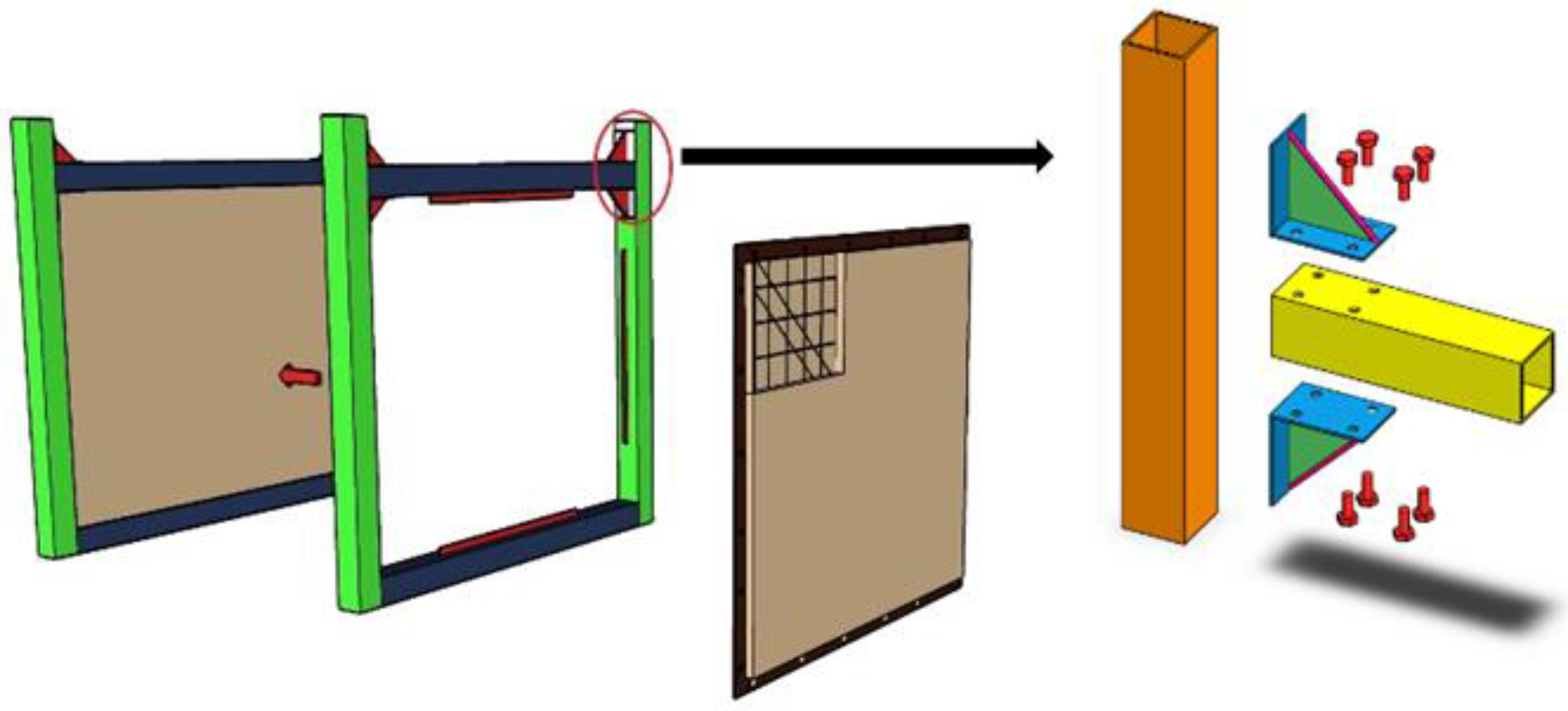
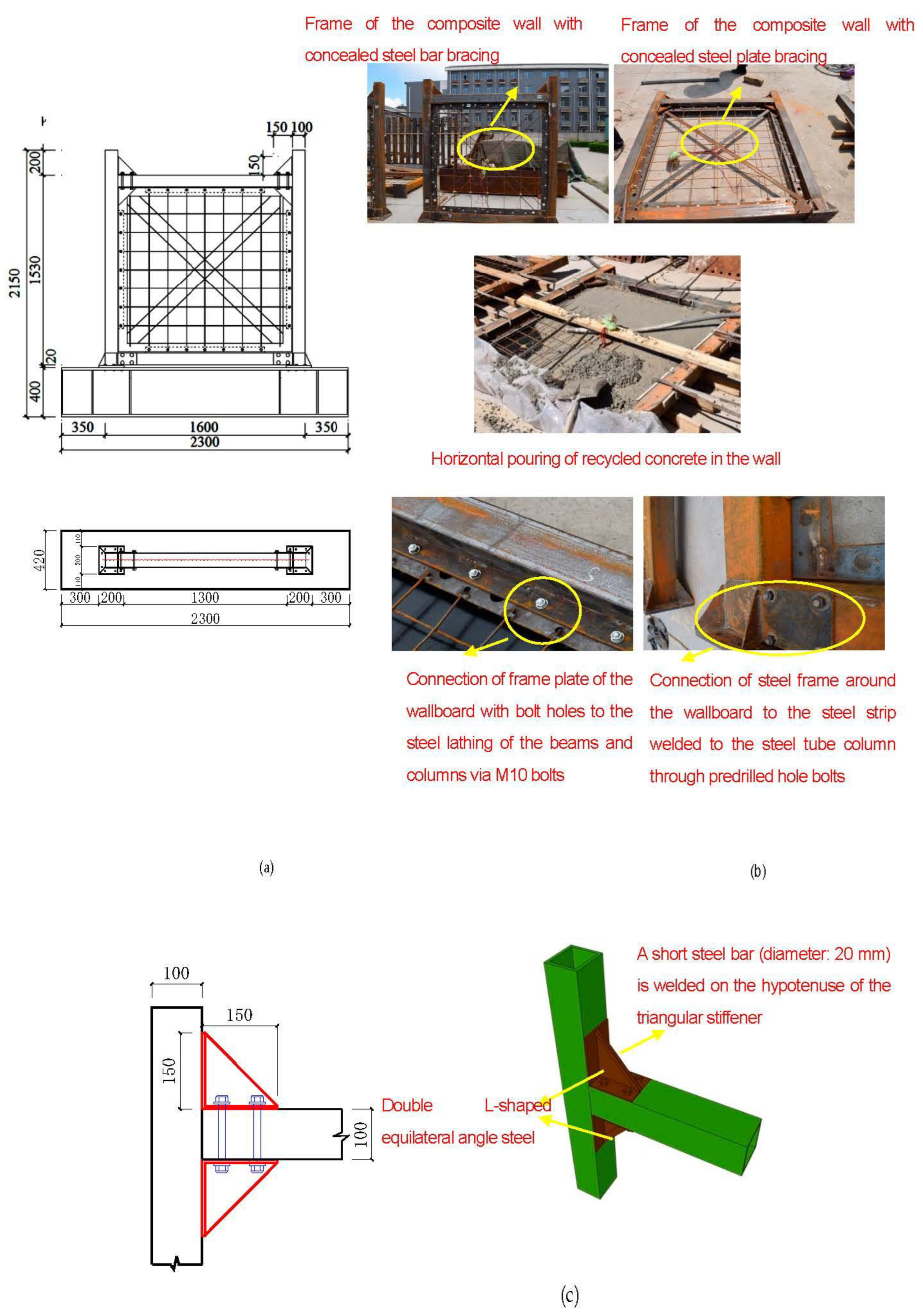
2. Composite-Shear Wall with Concealed Bracings in Steel-Tube Frame

Composite-shear walls with concealed bracings in steel-tube frames are earthquake-resistant wall units suitable for use in low-rise and multi-storey residential buildings. These shear walls are assembled from steel-tube frames and recycled concrete wallboards with concealed bracings.

The steel-tube frame was prepared by assembling steel-tube recycled concrete columns and beams following reinforced joints, whereby two equilateral steel angles are welded to the column at one end and bolted to the beam via the vertical bolt holes reserved at the other. It should be noted that triangularly shaped stiffening ribs, in which the hypotenuses are welded with short reinforcement bars (diameters: 20 mm), were welded to the centre of the steel angle [42]. The steel frame of the recycled concrete wallboard was composed of a frame steel plate, a two-way distribution bar, and concealed bracings. Bolt holes were retained in the frame steel plate which surrounded the wallboard to match the bolt holes on the steel lathings welded on the steel-tube beams and columns, as shown in Figure 1.

Six 1/2-scale composite shear wall test pieces were designed in our previous studies [34,35]. All test pieces had the same steel-tube frame structure. The dimensions and structural diagram of the test pieces are shown in Figure 2a, Figure 2b shows the fabrication process of the member and the installation position of the dark support, The diameter of the steel dark support used in the test pieces is 5 mm, and the thickness of the steel dark support is 4 mm.nd Figure 2c shows the geometry of the reinforcement joint and the connection to the beam and column, and the design parameters are listed in

Table 1. Design parameters of the composite shear wall.

Test Piece No.	Type of Concealed Bracing	Thickness of Wallboard	Axial Compression Ratio	Spacing between Reinforcement Bars	Reinforcement Ratio of the Distribution Bars
MX-1	Concealed steel bar bracing	60 mm	0.39	100 mm	0.33%
MX-2	Concealed steel plate bracing	60 mm	0.39	100 mm	0.33%
MX-3	Concealed steel bar bracing	60 mm	0.39	150 mm	0.22%
MX-4	Concealed steel plate bracing	60 mm	0.39	150 mm	0.22%
MX-5	Concealed steel bar bracing	60 mm	0.39	200 mm	0.16%
MX-6	Concealed steel plate bracing	60 mm	0.39	200 mm	0.16%

.

The concrete used in our study was prepared by mixing recycled coarse aggregates with particles (with diameters in the range of 5–10 mm), natural sand, Portland cement, water, mineral powder, fly ash, and water reducer in a stirrer at specific proportions. The measured average compressive strength of the standard recycled concrete cube was 43.8 MPa. The mix proportions of concrete are listed in

Table 2. Mix proportions of the recycled concrete.

Strength Grade	Amount of the Materials Used in the Recycled Concrete (kg m−3)
	Cement	Fly Ash	Mineral Powder	Sand	Recycled Aggregate	Water	Water Reducer
C40	369	79	79	841	841	181	3.5

. The mechanical properties of the steel used to prepare the test pieces are listed in

Table 3. Mechanical properties of steel.

Type of Steel	Plate Thickness (Diameter)/mm	Yield Strength fy/MPa	Tensile Strength fu/MPa	Elongation δ/%	Elastic Modulus E/MPa
Distribution bar/Concealed steel bar bracing	5	680	786	5.5	2.09 × 105
Frame steel plate/Connected steel lathings/Concealed steel plate bracing	4	309	467	25.27	2.11 × 105
Square steel tube	4	375	477	23.23	2.18 × 105

.

3. Numerical Simulation of the Seismic Performances of Test Pieces

To obtain the restoring force model of a composite shear wall with concealed bracings and a steel-tube frame, the study first evaluated the seismic performance of four test pieces used in our previous studies [34,35] using ABAQUS simulations. Subsequently, the reliability of the numerical simulation was validated by comparing the simulation and laboratory test results. Finally, the seismic performance of the virtual test pieces was obtained by numerical simulations. The seismic magnitude of the components in this paper is designed to be earthquake resistant to earthquakes of magnitude 8 and above.

3.1. Numerical Simulations and Validation of Seismic Performances of Test Pieces

(1)

Computation model

To obtain more test samples, the study designed only the four types of virtual test pieces in Table 1, which were classified into four groups, by referring to the actual test pieces, as shown in Table 1. Each group included seven virtual test pieces. The structures of all first-test pieces in each group were identical to those of the actual test pieces MX-1, MX-2, MX-3, and MX-4, listed in Table 1, which were renumbered as MX-1-1, MX-2-1, MX-3-1, and MX-4-1, respectively, in

Table 4. Parameters of the virtual test pieces.

Test Piece No.	Type of Concealed Bracing	Strength of Recycled Concrete	Thickness of Wallboard (mm)	Axial Compression Ratio	Spacing between the Distribution Bars (mm)
MX-1-1	Concealed steel bar bracing	C40	60	0.38	100
MX-1-2	Concealed steel bar bracing	C30	60	0.38	100
MX-1-3	Concealed steel bar bracing	C25	60	0.38	100
MX-1-4	Concealed steel bar bracing	C40	50	0.38	100
MX-1-5	Concealed steel bar bracing	C40	40	0.38	100
MX-1-6	Concealed steel bar bracing	C40	60	0.3	100
MX-1-7	Concealed steel bar bracing	C40	60	0.5	100
MX-2-1	Concealed steel plate bracing	C40	60	0.38	100
MX-2-2	Concealed steel plate bracing	C30	60	0.38	100
MX-2-3	Concealed steel plate bracing	C25	60	0.38	100
MX-2-4	Concealed steel plate bracing	C40	50	0.38	100
MX-2-5	Concealed steel plate bracing	C40	40	0.38	100
MX-2-6	Concealed steel plate bracing	C40	60	0.3	100
MX-2-7	Concealed steel plate bracing	C40	60	0.5	100
MX-3-1	Concealed steel bar bracing	C40	60	0.38	150
MX-3-2	Concealed steel bar bracing	C30	60	0.38	150
MX-3-3	Concealed steel bar bracing	C25	60	0.38	150
MX-3-4	Concealed steel bar bracing	C40	50	0.38	150
MX-3-5	Concealed steel bar bracing	C40	40	0.38	150
MX-3-6	Concealed steel bar bracing	C40	60	0.3	150
MX-3-7	Concealed steel bar bracing	C40	60	0.5	150
MX-4-1	Concealed steel plate bracing	C40	60	0.38	150
MX-4-2	Concealed steel plate bracing	C30	60	0.38	150
MX-4-3	Concealed steel plate bracing	C25	60	0.38	150
MX-4-4	Concealed steel plate bracing	C40	50	0.38	150
MX-4-5	Concealed steel plate bracing	C40	40	0.38	150
MX-4-6	Concealed steel plate bracing	C40	60	0.3	150
MX-4-7	Concealed steel plate bracing	C40	60	0.5	150

. The other six test pieces were obtained by adjusting the strength of the recycled concrete, thickness of the wallboard, and axial compression ratio. The parameters of the virtual test pieces are listed in Table 4.

The ABAQUS model of the virtual test piece is shown in Figure 3d. The steel-tube frame and recycled concrete wall were constructed using hexahedral units in the model. The distribution bars and diagonal tension bars were embedded directly in the model. A fixed boundary condition was imposed on the bottom surface, whereas the top face and two sides of the model were set as free surfaces. A fixed constraint in the normal and tangential directions was imposed between the steel frame and recycled concrete wall to simulate a bolt connection. However, during the calculation, the constraint in the normal or tangential directions became invalid once the tensile or shear stress between the steel frame and recycled concrete wall exceeded the tensile or shear strengths of the bolt. The steel tube frame and recycled concrete wall are all 3 mm thick.

(2)

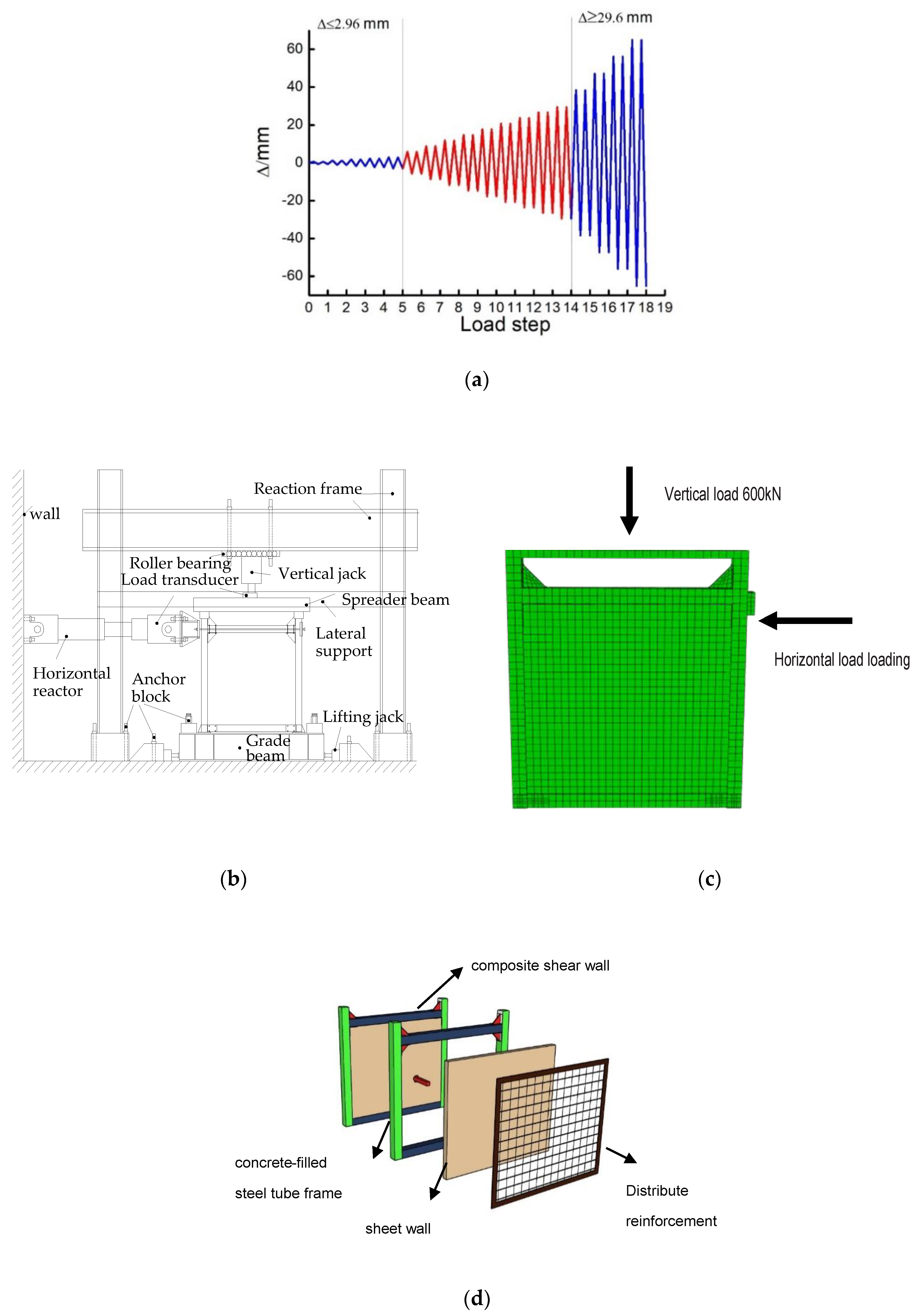
Loading scheme

The loading scheme used for the actual test pieces was adopted for the virtual test pieces as well (Figure 3). The displacement-controlled loading scheme was determined by referring to the Code for Seismic Design of Buildings [43,44]. Specifically, a vertical load of 600 kN was first applied at the centre of the top surface of the supported beam. This load was then distributed symmetrically to the top surfaces of the columns on both sides of the steel frame. The vertical load was maintained constant during the test. Subsequently, a low-cyclic reversed horizontal load was applied at the axis of the frame beams; the loading point was 1480 mm from the top surface of the foundation. During loading, the increments in the angular displacement were set to 1/2500 and 1/500 before the angular displacement of the test piece reached 1/500 and 1/50, respectively. After the angular displacement exceeded 1/50, the increment in angular displacement was set to 3/500. Each loading stage was repeated twice until extensive damage occurred in the test piece, or the horizontal load decreased to values less than 85% of the peak load. In the latter case, loading could not be applied to the test piece. Both cases signified the end of the test. In the case of the steel-tube frame, the displacement angle incurred during elastic deformation, which reached a maximum of 1/500, while that induced during elastic–plastic deformation was 1/50.

(3)

Constitutive relations and yield criteria

Three main constitutive models of concrete are commonly used in ABAQUS: smeared cracking, brittle cracking, and damage plasticity. The concrete plastic damage model considers the compressive plastic strain to be controlled by the plastic compressive yield surface. It also considers the damage effects of the material. It uses isotropic tensile and compressive plasticity to replace the inelastic properties of concrete, and can accurately simulate the structural behaviour and responses of concrete subjected to monotonic loading [45]. In this study, the concrete plastic damage model was used for simulation.

The plastic damage model of concrete in ABAQUS is a plastic-based damage model, and assumes that the concrete material mainly exhibits tensile cracking and compression fracture [45]. Its yield and failure are determined by the equivalent tensile plastic strain ${\tilde{\epsilon }}_t^{pl}$ and equivalent compressive plastic strain ${\tilde{\epsilon }}_c^{pl}$, respectively.

The concrete tensile damage curve is used to convert the cracking strain into plastic damage strain through the relationship between the failure stress and cracking strain, while the concrete compression damage curve is used to convert the inelastic strain into plastic strain for calculation. The calculation formulae for these two variables are expressed by Equations (1) and (2).

$${\tilde{\epsilon }}_t^{pl}={\tilde{\epsilon }}_t^{ck}-\frac{d_t}{\left(1-d_t\right)}\frac{{\sigma }_t}{E_0}$$

(1)

$${\tilde{\epsilon }}_c^{pl}={\tilde{\epsilon }}_c^{in}-\frac{d_c}{\left(1-d_c\right)}\frac{{\sigma }_c}{E_0}$$

(2)

where: ${\tilde{\epsilon }}_t^{ck}$ is the cracking strain, which is the total strain minus the elastic strain of the non-destructive material, ${\tilde{\epsilon }}_t^{ck}={\epsilon }_t-{\epsilon }_{0t}^{el}$, ${\epsilon }_{0t}^{el}={\sigma }_t/E_0$; ${\tilde{\epsilon }}_c^{in}$ is the compressive inelastic strain, which is the total strain minus the elastic strain of the lossless material, ${\tilde{\epsilon }}_c^{ck}={\epsilon }_c-{\epsilon }_{0c}^{el}$, ${\epsilon }_{0t}^{el}={\sigma }_c/E_0$; $d_t$ is the tensile damage variable, and $d_c$ is the compression damage variable. The concrete calculation parameters used in the simulation in this paper are shown in

Table 5. Simulation parameters.

Young’s Modulus	Poisson’s Ratio	Dilation Angle	Eccentricity	fbo/fco	k	Viscosity Parameter
34,500	0.2	30°	0.1	1.16	0.667	0.009

.

In this study, for both steel bars and steel plates, adopted the elastic strengthening model (i.e., the double-broken line model). The yield criterion is the von Mises yield criterion, and the strengthening criterion is the follow-up strengthening criterion. Simplifying the stress–strain relationship after the steel yields an oblique line with $E_s^{|}=0.01E_s$. The Poisson’s ratio was 0.3.

fbo/fco means that the biaxial limit is the ratio of the biaxial ultimate compressive strength to the uniaxial ultimate compressive strength, and the default value is 1.16 in this paper. The ratio k of the second stress constant of the tensile meridian plane to the compression meridian plane takes the default value of 0.667.

(4)

Finite Element Simulation Boundary Condition Setting

The boundary conditions of the model are relatively clear, and the bottom surface of the model base is defined as rigid. That is, all six degrees of freedom of the square steel tube column foot are constrained in ABAQUS. The axial load applied at the top of the frame column is constrained by coupling, and the horizontal center of the frame beam is subjected to repeated horizontal displacement with low cycle (Figure 3c), and coupling constraint is also used. During the finite element simulation of the model loading process, three analysis steps are set: initial analysis step (Initial) and subsequent analysis steps Step-1 (Static, General), Step-2 (Static, General).

In the finite element analysis simulation calculation, three analysis steps are defined, namely the initial analysis step (Initial), Step1 (Static, General), and Step-2 (Static, General). (1) Initial analysis step (Initial): It is mainly to set the boundary conditions in the component. For example, all six constraints of the column foot of the square steel tube column are constrained, that is, a rigid surface. (2) Step-1: The vertical concentrated load of 600 kN is mainly applied at the reference point on the top surface of the distribution beam, and the vertical load is evenly applied to the frame columns on both sides through the distribution beam through the distribution beam, and transferred to Step-2; (3) Step-2: The horizontal displacement is applied to the horizontal center of the specimen frame beam 1480 mm away from the foundation beam, and the unidirectional step-by-step loading is defined as the control of the horizontal displacement. Its loading step is cyclically loaded according to the amplitude of the experiment.

3.2. Analysis of the Computation Results and Validation

All 28 virtual test pieces were subjected to low-cyclic reversed loading simulations in ABAQUS according to the aforementioned loading scheme. The stress contour, failure morphology, hysteretic curve, and skeleton curve of each test piece were obtained from numerical simulations. For simplicity, the calculated results of the four virtual test pieces which yielded the same material and structure as the actual test pieces are listed herein and compared with the experimental test results.

(1)

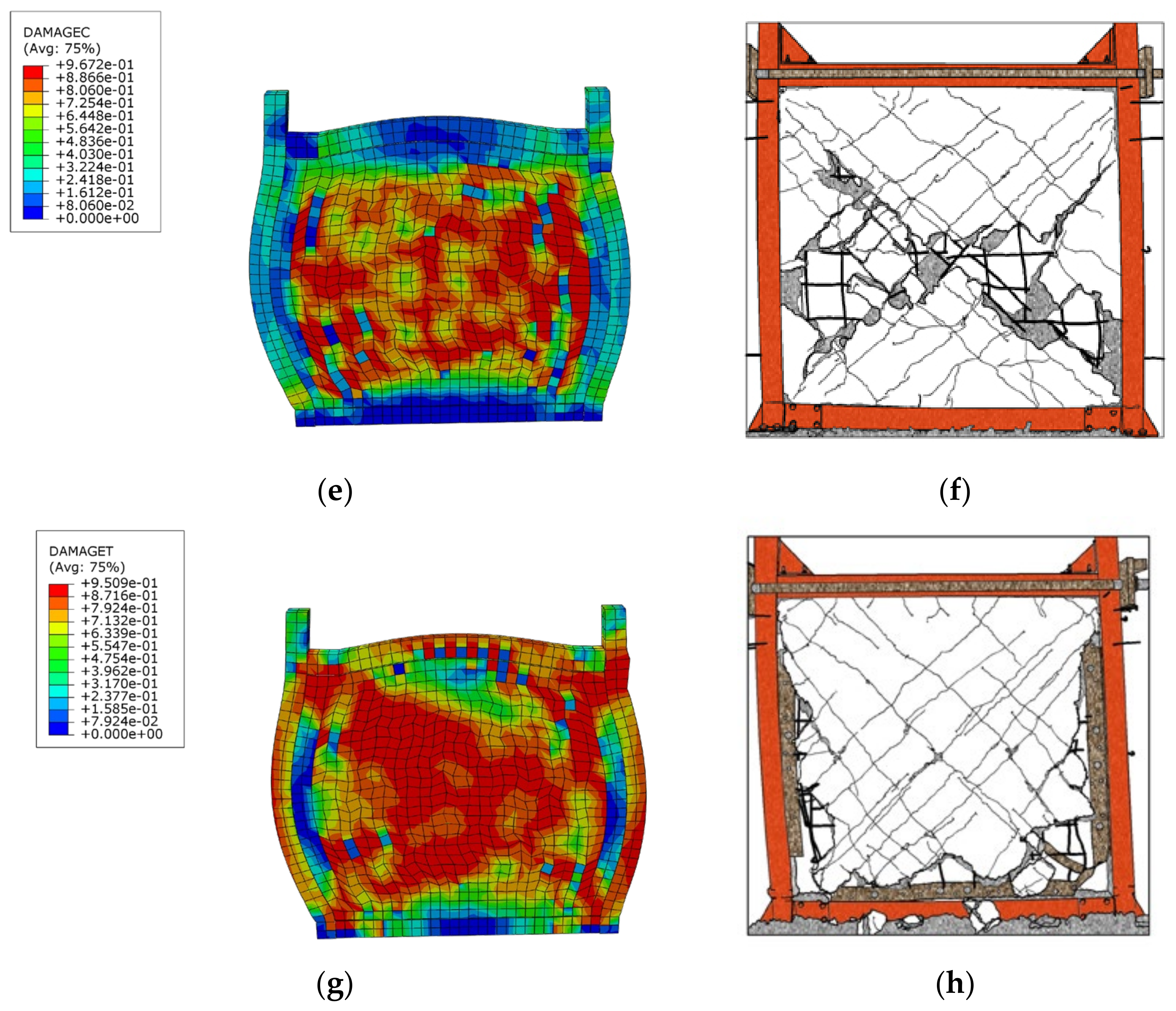
Failure morphology of the test pieces:

The stress contours of the virtual concrete-wall test pieces MX-1-1, MX-2-1, MX-3-1, and MX-4-1 are shown in Figure 4a,c,e,g, respectively. All four test pieces experienced different levels of shear yield. The failure morphologies of the actual test pieces MX-1, MX-2, MX-3, and MX-4 are shown in Figure 4b,d,f,h, respectively. The comparison between neighbouring images revealed similar failure morphologies among the four virtual test pieces and the corresponding actual test pieces. Specifically, the wallboard displayed shear failure, whereas the steel-tube column displayed bending failure. The horizontal resistance of the composite wall supported by steel reinforcements was at least 14.06% higher than that of the composite wall supported by a steel plate subjected to the same loading mode. The horizontal resistance of the composite wall supported by steel reinforcement is at least 6.26% higher than that of the composite wall supported by steel plate under the same loading mode, as is shown in

Table 6. Cumulative energy consumption of specimens at different stages.

Assembly Number	Peak Displacement (mm)	Peak Load (kN)
MX-1	14.56	1166.75
MX-2	13.78	1076.78
MX-3	14.22	1079.90
MX-4	12.18	1016.27

.

As shown in Figure 4 (The value range in the contour is between 0 and 1, which is close to 1, which indicates that the concrete damage is more serious there) [45], for the failure form and damage process of the component, the FE simulation using ABAQUS is consistent with the existing test results. The model first generates a large stress in the diagonal direction. As the horizontal displacement gradually increases, the damage range of the thin wall panel gradually extends along the diagonal line, thus forming a diagonal damage area. Finally, the thin wall panel is damaged in the core area and corners. The foot stress of the frame column was large. This finding is consistent with the test results which showed that the thin wall panel first suffered shear failure, and the steel-tube frame then suffered compression bending failure during the actual loading process of the specimen. That is, in the early stage of the test, the cross-inclined cracks of the thin wall panel continued to develop. As the displacement of the apex of the seismic element increased, the edge of the thin wall panel and the steel pipe frame were dislocated, the recycled concrete was crushed and peeled off, the edge connection structure was exposed, and no obvious damage occurred. When the specimen was damaged, the bottom part of the steel pipe column bulged and assumed the shape of a lantern.

As shown in Figure 4a that the plastic damage of concrete in the concrete compression zone at the corner of the member is the most serious, which is consistent with the actual damage of the member in Figure 4b.

Figure 4c shows that the damage value of the concrete at the four corners of the component is the largest, close to the maximum value of 1. This is consistent with the four corners of concrete falling off in the final failure of Figure 4d (that is, the concrete failure form at this place).

Figure 4f shows the final failure state of the component, with the concrete falling off in the middle and the concrete showing an “X”-shaped crack, which is consistent with the simulation shown in Figure 4e.

Figure 4h shows that the concrete failure of the member close to the frame column is the most severe, which is consistent with the simulation shown in Figure 4g.

(2)

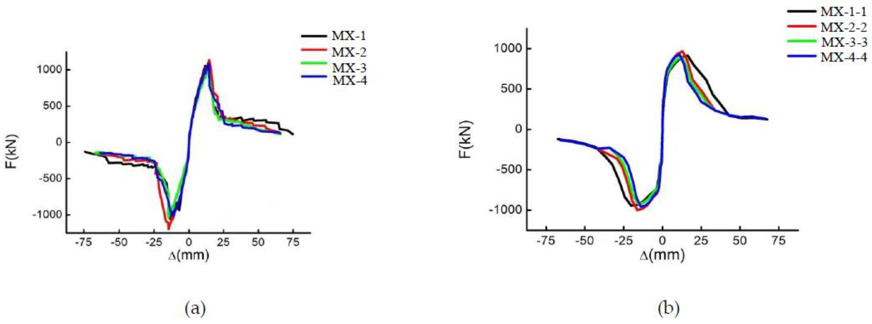
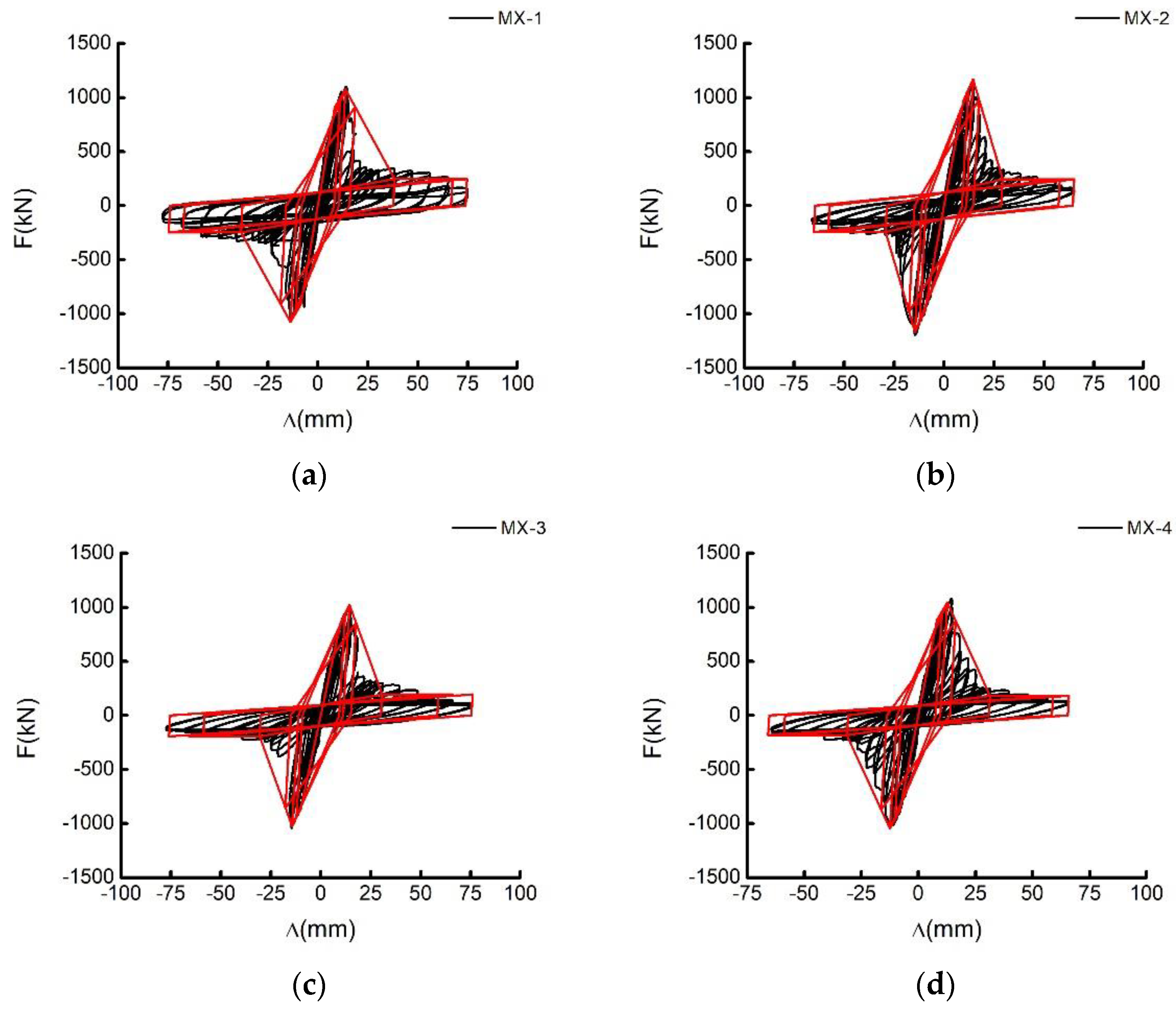
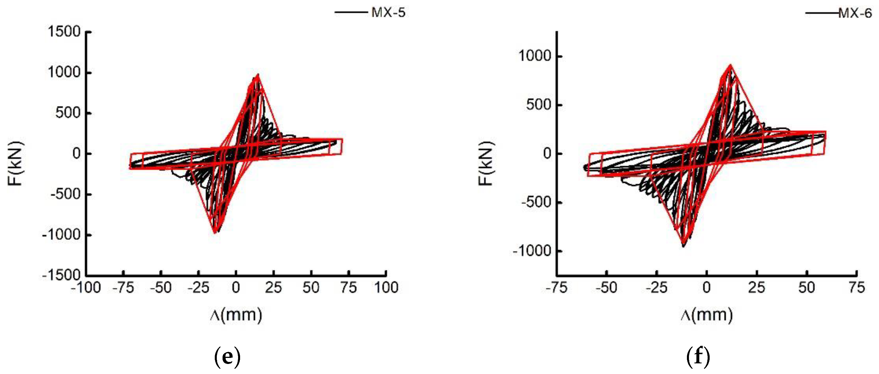
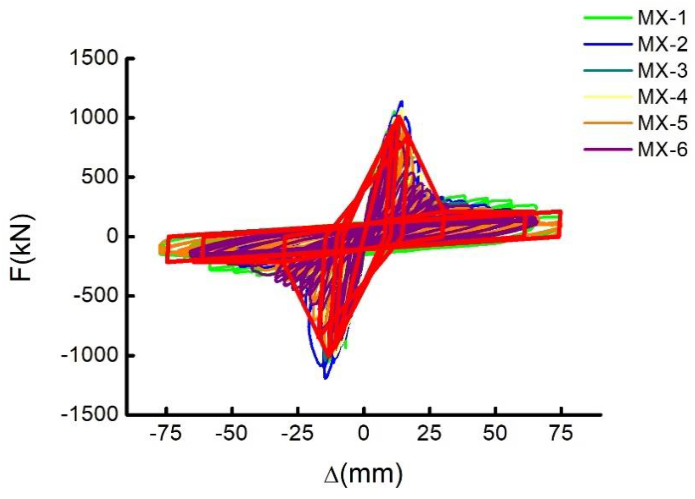
Hysteretic curve

The hysteretic curves of the virtual (MX-1-1, MX-2-1, MX-3-1, and MX-4-1) and actual test pieces (MX-1, MX-2, MX-3, and MX-4) are shown in Figure 5.

As shown in Figure 5, the hysteretic curves of the virtual test pieces agree well with those of the actual test pieces. In particular, the test pieces yield butterfly-shaped hysteretic curves. This feature indicates two seismic fortification lines in the composite-shear wall. In other words, owing to the seismic force, the wallboard of the test piece may be destroyed first, followed by the steel-tube frame.

Figure 5a–d shows that the simulated skeleton curve is relatively consistent with the measured curve in the early stage of loading. The hysteresis curve in the early stage of loading shows a nearly straight line, whether it is simulation or experiment. The measured curve is close to each other, and the hysteresis curve of the specimen shows an inverse S shape in both simulation and experiment. The hysteresis curve obtained from the simulation is also butterfly-shaped, which means that the components obtained from the simulation are also consistent with the experimental results. As shown in Figure 5a, the simulation results of component MX-1 deviate from the measured results by about 4.81%. Figure 5b shows that the simulation results of component MX-2 deviate from the measured results by about 5.91%. Figure 5c It is shown that the simulated result of component MX-3 deviates from the measured result by about 5.27%, and Figure 5d shows that the simulated structure of component MX-1 deviates from the measured structure by about 6.25%.

The simulated hysteretic curve fits well the experimental hysteretic curve, and the largest and smallest differences between them are 6.25% and 4.81%, respectively. Therefore, it is reliable to use ABAQUS to simulate effectively the mechanical characteristics of components.

(3)

Skeleton curve:

The skeleton curves of the virtual (MX-1-1, MX-2-1, MX-3-1, and MX-4-1) and actual test pieces (MX-1, MX-2, MX-3, and MX-4) are shown in Figure 6a,b, respectively. As shown in Figure 6, the skeleton curves of the virtual test pieces agree well with those of the actual test pieces.

As shown in Figure 6, the skeleton curve of the test piece can be categorised into four segments. When the composite wall reaches its maximum displacement point, the inter-storey displacement angle is approximately 1/59. When the test piece is destroyed, the composite wall degrades into a steel frame structure, and the inter-storey displacement angle is approximately 1/23. This angle is used as a control point to determine the structural collapse. In addition, the yield and peak loads of the structure decrease with increasing spacing between the distribution bars. Additionally, employing diagonal steel bar bracings instead of diagonal steel plate bracings yield an increased collapse resistance to the entire structure. Therefore, the use of diagonal steel bar bracings yields a more reasonable design, and helps improve the ductility of the structure. The simulated skeleton loop curve in Figure 6 deviates from the experimental skeleton curve with values in the range of 4.81–6.25% (note: 1/53, 1/29 represent the interlayer displacement to which the member is loaded. The interlayer displacement is the ratio of the maximum interlayer y displacement of the vertical member to the average interlayer displacement).

As shown from the above analyses, the numerical simulation of the composite shear wall performed using the FE software ABAQUS yielded results that were highly consistent with the experimental test data. In other words, the mechanical performance of the composite-shear wall is accurately reflected by the FE simulation outcomes.

(4)

Effects of varying parameters on seismic performance of test pieces:

Figure 7 shows the hysteretic curves of the other virtual test pieces. As shown in the figure, reducing the strength of the recycled concrete or the thickness of the wallboard results in a lower bearing capacity of the composite wall. In addition, the bearing capacity and lateral displacement of the composite wall improve considerably when the axial compression ratio decreases.

As shown in Figure 7a, parameter changes were performed on the specimen MX-1. The changed parameters are recycled concrete strength, concrete slab thickness, and axial compression ratio. With the decrease of the strength of the recycled concrete, the bearing capacity of the composite wall decreases, so when C40 is selected, the strength of the specimen is the highest. The bearing capacity of the component decreases with the thickness of the concrete wall panel, indicating that the specimen has the best performance when the strength of the concrete panel is 60 mm. In addition, with the decrease of the axial compression ratio strength, the bearing capacity of the specimen increases significantly, so when the axial compression ratio is 0.3, the bearing capacity of the specimen is the largest.

Figure 7b–d also carried out the same parameter changes for the specimens MX-2-MX-4, respectively. The conclusions reached are consistent with Figure 7a.

The hysteretic curves of the composite walls shown in Figure 7 are all butterfly-shaped, and can be roughly divided into two developmental stages. The slope of the first stage of the curve (that is, the curve part in which the concrete wall and the steel pipe frame function together) is steeper. The slope of the hysteresis curve after the concrete wall is damaged is relatively gentle. Figure 7 shows that the hysteretic curve obtained by numerical simulations is basically consistent with that obtained experimentally, and proves that the numerical simulations conducted herein were effective.

4. Establishment and Validation of the Restoring Force Model

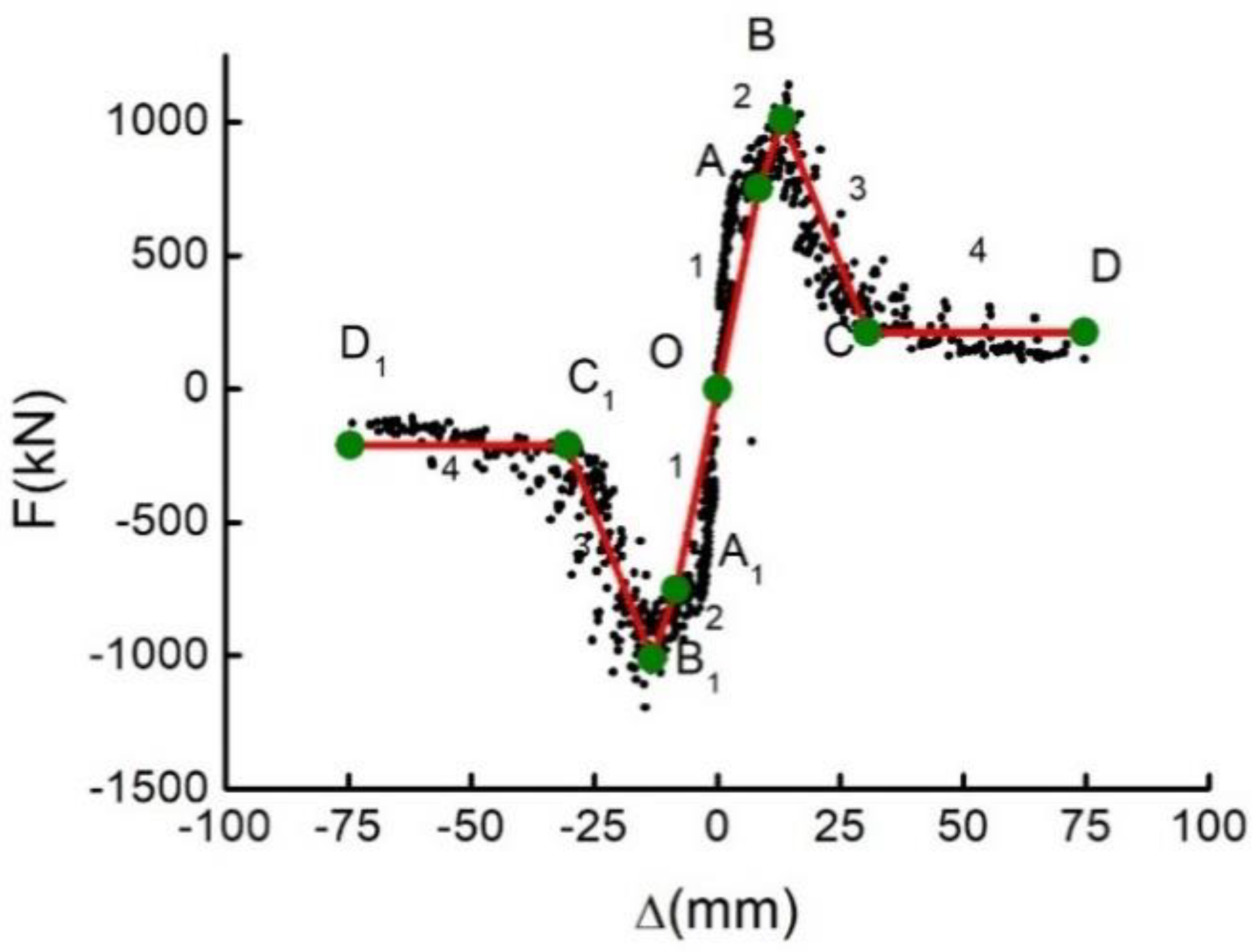
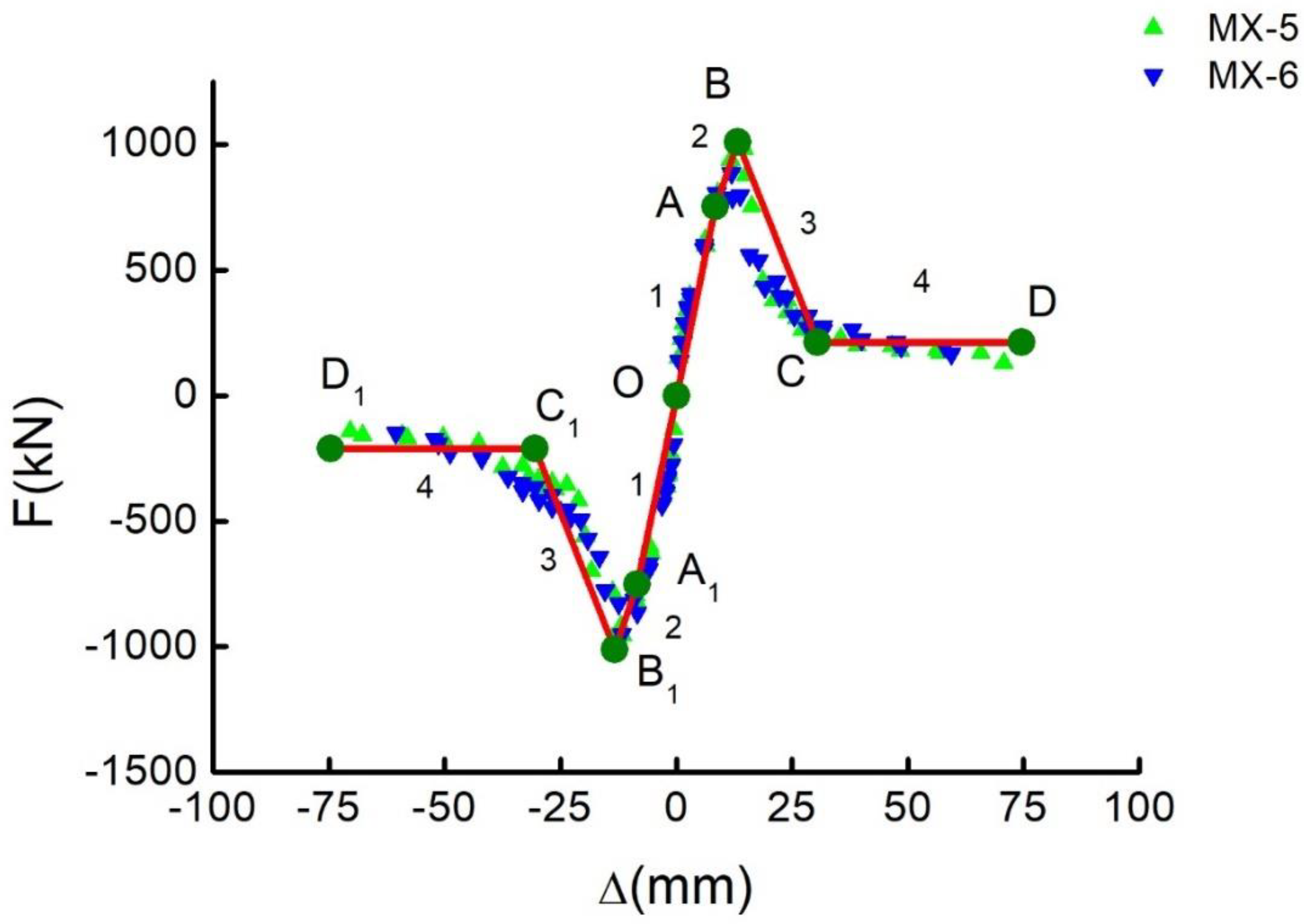
4.1. Construction of the Skeleton Curve

Figure 8 shows the general skeleton curve of the virtual test piece. A reasonable pattern is shown in Figure 8, in which the test piece reaches the yield points A,A₁, B,B₁, C,C₁ and D,D₁, consecutively. Therefore, the skeleton curve of this type of composite wall can be represented by a quadric-linear curve.

Each segment of the skeleton curve shown in Figure 8 can be represented by the following Equations (3)–(9):

$$F=88.71\Delta$$

(3)

$$F=53.35\Delta +300.17$$

(4)

$$F=53.35\Delta -300.17$$

(5)

$$F=-46.34\Delta +1626.80$$

(6)

$$F=-46.34\Delta -1626.80$$

(7)

$$F=211.48$$

(8)

$$F=-211.48$$

(9)

As shown in Figure 8, the entire skeleton curve is segmented into four segments. The first segment encompasses the elastic stage during which cracks are formed on the wallboard, and extends until the occurrence of definite yield. The second segment encompasses the strengthened yield stage, which starts from the definite yield point and ends at the ultimate load point of the composite wall with frames. During this stage, the bearing capacity of the composite wall continues to increase, and the ultimate load of the composite wall represents the limiting load of the first seismic line of defence. When the effect of the earthquake is within the ultimate bearing capacity of the composite wall, the composite wall primarily relies on its bearing capacity to resist the earthquake. In the third stage, the bearing capacity of the composite wall starts to decrease substantially, whereas the function of the wallboard gradually fails. When the effect of the earthquake exceeds the ultimate bearing capacity of the composite wall, the seismic energy is absorbed by the composite wall primarily through elastic–plastic energy dissipation to prevent structural collapse. In the final stage, the elastoplastic displacement of the steel tube-recycled concrete frame continues to increase. The errors between the four-line curve shown in Figure 8 and the experimental skeleton curve are all less than 5.92%, so the proposed four-line curve can be well fitted and used to represent the skeleton curve of this type of specimen.

The skeleton curve obtained through fitting in this study is further validated by comparison with the skeleton curves of the actual test pieces MX5 and MX6, as shown in Figure 9.

As shown in Figure 9, the fitted skeleton curve of the 28 virtual test pieces agrees well with the skeleton curve of the actual test piece, thereby validating the quadric-linear skeleton curve developed in this study.

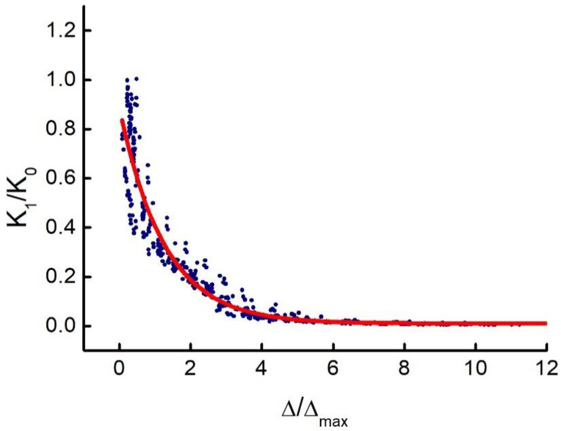
4.2. Stiffness Degradation Curve

The unloading stiffness of the composite wall degrades as the horizontal displacement increases. A non-dimensional analysis has been performed on the unloading stiffness to investigate the variation trend. As shown in Figure 10, $K_i$ can be calculated using Equation (10), where $K_0$ is the initial stiffness determined from the regression equation of the skeleton curve, $\Delta$ is the displacement associated with each peak load, and ${\Delta }_{max}$ is the displacement associated with the maximum load of the test piece.

$$K_i=\frac{\left|+F_i\right|+\left|-F_i\right|}{\left|+{\Delta }_i\right|+\left|-{\Delta }_i\right|}$$

(10)

Herein, $i$ is the number of loading cycles, $K_i$ is the secant stiffness within the $i$th loading cycle, $F_i$ is the peak load within the $i$th loading cycle, and + and − represent the positive and negative directions of the horizontal force, respectively.

Figure 10 shows the stiffness degradation curve of the composite wall.

Figure 10 shows the strong exponential relationship between K₁/K₀ and Δ/Δmax (Among them, in the range of 0.83 < K₁/K₀ < 0.06 and 0.32 < Δ/Δmax < 11.61, it shows a good effect). Therefore, this curve can be fitted using an exponential function. The regression function for this type of structure can be expressed by Equation (11):

$$\frac{K_1}{K_0}=0.87785e^{\frac{-\frac{\Delta }{{\Delta }_{max}}}{1.25092}}+0.01066$$

(11)

In addition, as shown in Figure 10, the composite wall exhibits a large initial stiffness. However, the stiffness values of the test pieces decrease rapidly as the wallboard begins to crack. When the wallboard is severely damaged and fails to function, the beam and column of the frame continue to withstand the load, resulting in a continuous reduction in the stiffness at a substantially slower rate

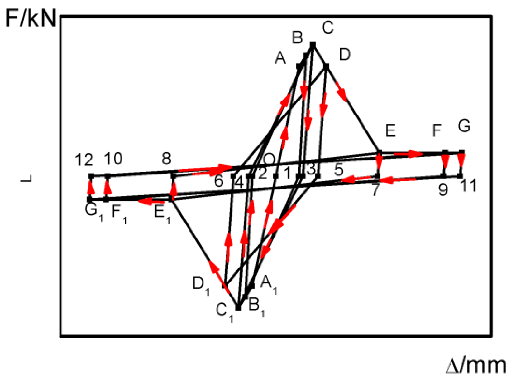
4.3. Establishment of the Restoring Force Model

After analysing the skeleton curve and stiffness degradation curve, the restoring force characteristics can be described by a degradation quadric-linear model (refer to Figure 11) by considering different failure stages of the test piece and the peak-oriented trend during reverse loading.

Referring to Figure 11, the restoring force model is described as follows:

The loading is along O-A-O-A1, and the specimen is in the elastic stage at this time, where A and A1 are the positive and negative yield points of the specimen.

Loading and unloading are along A-B-1-B1-2-B, at this time the specimen is in the elastic-plastic stage and has not reached the limit load point. The coordinates of B and B1 are 0.5 times the coordinates of the peak load point of this section.

Loading and unloading are along B-C-3-C1-4-C, when the specimen reaches the maximum load from the strengthening stage. where C and C1 are the forward and reverse peak load points.

Loading and unloading are along C-D-5-D1-6-D, at this time, the load of the specimen begins to decrease, and the wall gradually loses its bearing capacity. The coordinates of D and D1 are 0.8 times the coordinates of the peak load point of this section.

Load and unload along D-E-7-E1-8-E, when the load of the specimen drops to the lowest point.

Loading and unloading are along E-F-9-F1-10-F, and the bearing capacity of the specimen does not change with the increase of displacement. Among them, the abscissa values of F and F1 take 0.8 times the abscissa of the peak load point of this section.

Loading and unloading are along F-G-11-G1-12-G, and the bearing capacity of the specimen reaches the failure load at this time. Among them, G and G1 are the load points when the specimen finally fails.

Points 1–12 are the points of unloading to zero load, and their coordinate positions can be determined by the fitting curve of unloading stiffness.

Among them, the points B, D, F, G, B1, D1, F1, and G1 are the load dump points, and their coordinates are determined according to the above rules.

As shown in Figure 11, the restoring force model is established based on the following rules:

• The loading curve is traced along the O-A-O-A1 path. The test piece is still in the elastic region, and A and A1 are the positive and negative yield points of the test piece, respectively.
• The loading and unloading curves are traced along the A-B-1-B1-2-B path. The test piece is in the elastoplastic region before reaching the ultimate load point. The coordinates of B and B1 are regarded as 0.5 times the coordinates of the peak load point in this segment. Moreover, 1 and 2 are the forward and reverse zero-loading points, respectively. Their ordinates are calculated from the unloading stiffness fitting curve.
• The loading and unloading curves are along the path B-C-3-C1-4-C. Within this segment, the test piece transitions from the hardening to the peak stage. C and C1 are the forward and reverse peak-loading points, respectively. Furthermore, 3 and 4 are the forward and reverse zero-loading points, respectively. Their ordinates are calculated from the unloading stiffness fitting curve.
• The loading and unloading curves are along the path C-D-5-D1-6-D. Within this segment, the bearing capacity of the test piece decreases rapidly, which indicates the failure stage. The coordinates of D and D1 are considered to be equal to 0.8 times those of the peak-loading points. Further, 5 and 6 are the forward and reverse zero-loading points, respectively. Their ordinates are calculated from the unloading stiffness fitting curve.
• The loading and unloading curves are along the path D-E-7-E1-8-E. The bearing capacity of the test piece reaches the ultimate limit. E and E1 are the respective points at which the forward and reverse loads decrease suddenly. Moreover, 7 and 8 are the forward and reverse zero-unloading points, respectively. Their ordinates are calculated from the unloading stiffness fitting curve.
• The loading and unloading curves are along the E-F-9-F1-10-F path. During this stage, the bearing capacity of the test piece remains constant as a function of displacement. The abscissas of F and F1 are regarded to be equal to 0.8 times that of the peak load point. Further, 9 and 10 are the forward and reverse zero-loading points, respectively. Their ordinates are calculated from the unloading stiffness fitting curve.
• The loading and unloading curves are along the path F-G-11-G1-12-G. The test piece has now undergone failure. G and G1 are the failure loading points, and 11 and 12 are the forward and reverse zero-loading points, respectively. Their ordinates are calculated from the unloading stiffness fitting curve.
• Points B, D, F, G, B1, D1, F1, and G1 shown in the figure represent sudden decreases in the load. The coordinates of these points are determined based on the rules listed above.

4.4. Validation of Restoring Force Model

The hysteretic curves of the six actual test pieces and the restoring force model of 28 virtual test pieces are plotted on the same coordinate system (Figure 12). As shown in the figure, the hysteretic curves and restoring force model reveal the same loading and unloading trends. Therefore, the quadric-linear restoring force model proposed herein can accurately characterise the seismic performance of the composite shear wall investigated in this study.

Loading is carried out using Equations (3)–(9) fitted by the proposed restoring force model, and unloading is carried out according to the above-mentioned rules in Figure 11. The restoring force model of each specimen is shown in Figure 12a–f. The restorative force model is in good agreement with the hysteresis curve as a whole. The deviations between the hysteresis curve and the fitted restorative force model in Figure 4a–f are 6.37%, 5.23%, 7.36%, 6.02% 6.71%, and 8.03%.

The quadric-linear restoring force model proposed in this study is in agreement with the experimental data. Figure 13 shows that the MX-2 member exceeds the maximum horizontal force of the restoring force model by approximately 5.23%, and MX-6 is lower than the maximum level of the restoring force model. The force is approximately 8.03%. The deviation values of the remaining components are all less than 8.03%. Hence, the four linear restoring force models can be used to study the mechanical characteristics of the relevant composite walls.

5. Conclusions

On the basis of the low-cycle, repeated load test of the composite-shear wall with a built-in dark support steel pipe frame, the numerical simulation calculations of the low-cycle, repeated load actions of different virtual specimens were conducted using ABAQUS, and the stress cloud diagram and failure of each specimen were obtained. The morphology and the hysteretic and skeleton curves were generated. On this basis [34,35], the calculation formula of stiffness degradation was obtained according to the regression analysis of the stiffness degradation data, and the four-fold line restoring force model of the composite shear wall with built-in dark support steel tube frame was established.

• In previous studies [34,35], low-cyclic, reversed loading tests were performed on six 1/2 scale composite-shear wall test pieces with concealed bracings and steel tube frames. Based on these results, the study performed low cyclic reversed loading simulations of 28 virtual test pieces in ABAQUS. The stress contour, failure morphology, hysteretic curve, and skeleton curve of each test piece were obtained from numerical simulations. By performing regression analysis on the stiffness degradation data, the study obtained the stiffness degradation function, and then developed a quadric-linear restoring force model for a composite shear wall with a steel tube frame and concealed bracings.
• The study analyzed the effects of different controlling parameters on the seismic performance of the structure by modifying the wallboard thickness, strength of the recycled concrete, and axial compression ratio of the composite shear wall model with concealed bracings and a steel tube frame. The results indicated that the bearing capacity of the composite shear wall decreased as a function of the axial compression ratio. However, increasing the wallboard thickness and the strength of the recycled concrete leads to increased bearing capacity and lateral stiffness of the composite-shear wall.
• The composite-shear wall with a steel-tube frame and concealed bracings exhibited excellent seismic performance. This structure can be used as an earthquake-resistant component to construct buildings with high-seismic intensity in rural areas.

References

- Rodgers, J.E.; Mahin, S.A. Effects of connection fractures on global behavior of steel moment frames subjected to earthquakes. J. Struct. Eng. 2006, 132, 78–88. [Google Scholar] [CrossRef]
- Li, W. Seismic performance of CFST column to steel beam joint with RC slab: Joint model. J. Constr. Steel Res. 2012, 73, 66–79. [Google Scholar] [CrossRef]
- Xu, S.Y.; Zhang, J. Axial–shear–flexure interaction hysteretic model for RC columns under combined actions. Eng. Struct. 2012, 34, 548–563. [Google Scholar] [CrossRef]
- Penizen, J. Dynamic response of elasto-plastic frames. J. Struct. Div. ASCE 1962, 88, 1322–1340. [Google Scholar] [CrossRef]
- Clough, R.W.; Johnston, S.B. Effect of stiffness degradation on earthquake ductility requirements. In Proceedings of the 2nd Japan Earthquake Engineering Symposium, Tokyo, Japan, 1966. [Google Scholar]
- Sucuoglu, H.; Erberik, A. Energy-based hysteresis and damage models for deteriorating systems. Earthq. Eng. Struct. Dyn. 2004, 33, 69–88. [Google Scholar] [CrossRef]
- Shi, Y.; Wang, M.; Wang, Y. Experimental and constitutive model study of structural steel under cyclic loading. J. Constr. Steel Res. 2011, 67, 1185–1197. [Google Scholar] [CrossRef]
- Wang, M.; Shi, Y.; Wang, Y. Equivalent constitutive model of steel with degradation and damage. J. Constr. Steel Res. 2012, 79, 101–114. [Google Scholar] [CrossRef]
- Takeda, T.; Sozen, M.A.; Nielson, N.N. Reinforced concrete response to simulated earthquakes. J. Struct. Div. ASCE 1970, 96, 2557–2572. [Google Scholar] [CrossRef]
- Lignos, D.G. Sidesway Collapse of Deteriorating Structural System under Seismic Excitations. Ph.D. Thesis, Stanford University, Stanford, CA, USA, 2008. [Google Scholar]
- Park, Y.J.; Reinhorn, A.M.; Kunnath, S.K. IDARC: 1987 Inelastic Damage Analysis of Reinforced Concrete Frame-Shear-Wall Structures; Technical Report No. NCEER-87-0008; State University of New York: Buffalo, NY, USA, 1987. [Google Scholar]
- Song, J.K.; Pincheira, J.A. Spectral displacement demands of stiffness and strength degrading systems. Earthq. Spectra 2000, 16, 817–851. [Google Scholar] [CrossRef]
- Ibarra, L.F.; Medina, R.A.; Krawinkler, H. Hysteretic models that incorporate strength and stiffness deterioration. Earthq. Eng. Struct. Dyn. 2005, 34, 1489–1511. [Google Scholar] [CrossRef]
- Mostaghel, N. Analytical description of pinching, degrading hysteretic systems. J. Eng. Mech. 1999, 125, 216–224. [Google Scholar] [CrossRef]
- Della, C.G.; de Matteis, G.; Landolfo, R. Seismic analysis of MR steel frames based on refined hysteretic models of connections. J. Constr. Steel Res. 2002, 58, 1331–1345. [Google Scholar] [CrossRef]
- Ramberg, W.; Osgood, W.R. Description of Stress-Strain Curves by Three Parameters; Technical Note; NACA: Washington, DC, USA, 1943; Volume 902.
- Charalampakis, A.E.; Koumousis, V.K. Identification of Bouc–Wen hysteretic systems by a hybrid evolutionary algorithm. J. Sound Vib. 2008, 314, 571–585. [Google Scholar] [CrossRef]
- Wang, M. Damage and Degradation Behaviors of Steel Frames under Severe Earthquake. Ph.D. Thesis, Tsinghua University, Beijing, China, 2013. (In Chinese). [Google Scholar]
- Amde, A.M.; Mirmiran, A. A new hysteresis model for steel members. Int. J. Numer. Methods Eng. 1999, 45, 1007–1023. [Google Scholar] [CrossRef]
- Sivaselvan, M.V.; Reinhorn, A.M. Hysteretic models for deteriorating inelastic structures. J. Eng. Mech. 2000, 126, 633–640. [Google Scholar] [CrossRef]
- Wang, Q.; Shao, Y. Compressive performances of concrete filled Square CFRP-Steel Tubes (S-CFRP-CFST). Steel Compos. Struct. 2014, 16, 455–480. [Google Scholar] [CrossRef]
- Wang, Q.-L.; Li, J.; Shao, Y.-B.; Zhao, W.-J. Flexural Performances of Square Concrete Filled CFRP-Steel Tubes (S-CF-CFRP-ST). Adv. Struct. Eng. 2015, 18, 1319–1344. [Google Scholar] [CrossRef]
- Yongbo, S.; Qingli, W. Flexural performance of circular concrete filled CFRP-steel tubes. Adv. Steel Constr. 2015, 11, 127–149. [Google Scholar]
- Zhang, Y.; Shi, H. Hysteretic Model for Flexure-shear Critical Reinforced Concrete Columns. J. Earthq. Eng. 2017, 22, 1639–1661. [Google Scholar] [CrossRef]
- Du, G.-F.; Bie, X.-M.; Li, Z.; Guan, W.-Q. Study on constitutive model of shear performance in panel zone of connections composed of CFSSTCs and steel-concrete composite beams with external diaphragms. Eng. Struct. 2018, 155, 178–191. [Google Scholar] [CrossRef]
- Du, G.; Juan, J.; Zhang, J.; Li, Y.; Zhang, J.; Zeng, L. Experimental study on hysteretic model for L-shaped concrete-filled steel tubular column subjected to cyclic loading. Thin-Walled Struct. 2019, 144, 106278. [Google Scholar] [CrossRef]
- Yang, T.; Wang, S.-L.; Liu, W. Restoring-force model of modified RAC columns with silica fume and hybrid fiber. J. Cent. South Univ. 2017, 24, 2674–2684. [Google Scholar] [CrossRef]
- Papadopoulos, V. Numerical and Experimental Investigations of Nonlinear Behavior of RC Member and Slab-Column Assemblies in Bridges. Master’s Thesis, University of California, San Diego, CA, USA, 2015. [Google Scholar]
- Zhao, J.; Dun, H. A restoring force model for steel fiber reinforced concrete shear walls. Eng. Struct. 2014, 75, 469–476. [Google Scholar] [CrossRef]
- Yan, C.; Yang, D.; Jia, J.; Ma, Z.J. Hysteretic model of SRUHSC column and SRC beam joints considering damage effects. Mater. Struct. 2017, 50, 88. [Google Scholar] [CrossRef]
- Sigariyazd, M.A.; Joghataie, A.; Attari, N.K.A. Analysis and design recommendations for diagonally stiffened steel plate shear walls. Thin-Walled Struct. 2016, 103, 72–80. [Google Scholar] [CrossRef]
- Ma, H.; Xue, J.; Zhang, X.; Luo, D. Seismic performance of steel-reinforced recycled concrete columns under low cyclic loads. Constr. Build. Mater. 2013, 48, 229–237. [Google Scholar] [CrossRef]
- Ma, H.; Dong, J.; Liu, Y.; Yang, D. Cyclic loading tests and shear strength of composite joints with steel-reinforced recycled concrete columns and steel beams. Eng. Struct. 2019, 199, 109605. [Google Scholar] [CrossRef]
- Jia, S.; Cao, W.; Zhang, Y. Low reversed cyclic loading tests for integrated precast structure of lightweight wall with single-row reinforcement under a lightweight steel frame. R. Soc. Open Sci. 2018, 5, 181965. [Google Scholar] [CrossRef]
- Jia, S.; Cao, W.; Ren, L. Experimental study on seismic performance for fabricated composite structure of lightweight steel frame-lightweight wall with concealed support. J. Build. Struct. 2018, 39, 48–57. [Google Scholar] [CrossRef]
- Park, R. Evaluation of ductility of structures and structural assemblages from laboratory testing. Bull. N. Z. Natl. Soc. Earthq. Eng. 1989, 22, 155–166. [Google Scholar] [CrossRef]
- Lykidis, G.C.; Spiliopoulos, K.V. An efficient numerical simulation of the cyclic loading experiments on RC structures. Comput. Concr. 2014, 13, 343–359. [Google Scholar] [CrossRef]
- De Maio, U.; Greco, F.; Leonetti, L.; Blasi, P.N.; Pranno, A. A cohesive fracture model for predicting crack spacing and crack width in reinforced concrete structures. Eng. Fail. Anal. 2022, 139, 106452. [Google Scholar] [CrossRef]
- Suizi, J.; Wanlin, C.; Zibin, L. Experimental study on seismic performance of a low-energy consumption composite wall structure of a pre-fabricated lightweight steel frame. R. Soc. Open Sci. 2019, 6, 181965. [Google Scholar] [CrossRef] [PubMed]
- Jia, P.; Zhao, W.; Du, X.; Chen, Y.; Zhang, C.; Bai, Q.; Wang, Z. Study on ground settlement and structural deformation for large span subway station using a new pre-supporting system. R. Soc. Open Sci. 2019, 6, 181035. [Google Scholar] [CrossRef]
- Lei, B.; Liu, H.; Yao, Z.; Tang, Z. Experimental study on the compressive strength, damping and interfacial transition zone properties of modified recycled aggregate concrete. R. Soc. Open Sci. 2020, 6, 190813. [Google Scholar] [CrossRef] [PubMed]
- Jia, S.; Cao, W.; Wang, R.; Liu, W.; Ren, L. Seismic test on fabricated composite structure of Lightweight steel frame–thin slab for low- rise housing. J. Southeast Univ. 2018, 48, 323–329. (In Chinese) [Google Scholar] [CrossRef]
- GB 50011-2010; Code for Seismic Design of Buildings. Standards Press of China: Beijing, China, 2016. (In Chinese)
- GBT 50081-2002; Ordinary Concrete Mechanics Performance Test Method Standard. China Building Industry Press: Beijing, China, 2002. (In Chinese)
- Abaqus, F. ABAQUS Analysis User’s Manual 6.14-EF; Dassault Systems Simulia Corp.: Providence, RI, USA, 2014. [Google Scholar]