LES Analysis of the Effect of Snowdrift on Wind Pressure on a Low-Rise Building

Abstract

This paper presents a comparative study of the distribution of wind pressure acting on a low-rise building roof with or without snowdrift through the Large-Eddy simulation (LES) method. Firstly, based on previous wind-blowing snow experiments, the stable snowdrift models were obtained by reverse technique. Secondly, the methodology of LES numerical simulation was introduced, where sensitivity analyses were conducted to determine a more reasonable grid configuration and data sampling time. Meanwhile, the numerical validation was also verified by comparing it with the previous PIV database. Finally, the wind pressure acting on the building’s roof with or without snowdrift were systematically compared and analyzed. It was found that the snow cover significantly restrains the size of the separation bubble and makes is lcoated earlier on the roof, which leads to the increasing passing velocity in the region near the roof. Meanwhile, the area-averaged pressure coefficient in the windward region (x/H < 0.5) for the snowdrift roof will be significantly amplified, especially for the fluctuating pressure, the maximum value of the Relative Difference even reaches 40%. Additionally, according to the POD analysis, the snowdrift causes the fluctuating wind energy to concentrate near the windward side of the roof. Therefore, more attention should be paid to the wind pressure in the windward region when the snowdrift is formed on the roof.

1. Introduction

In snowy regions, wind-induced snow drift will cause uneven snow loads on the roofs of buildings, and it may modify the original roof shape to some extent and leads to the vibration of airflow around them [1,2]. Therefore, the distribution of the wind load on the roofs of buildings will be altered correspondingly, and this issue is rarely explored.

Wind loads acting on low-rise buildings have always been a research hotspot in wind engineering, and many studies have been carried out through field observation, wind tunnel experiments, and numerical simulation. Research factors are mainly included in the following three categories. (i) The overall or local geometric topology changes to the building (such as aspect ratio, roof slope, span, etc.; partial roof ancillary facilities, solar panels, parapets, deflectors, openings on the building surface, etc.); (ii) the characteristics of oncoming wind fields (such as turbulence intensity, integration scale, Reynolds number, wind direction angle, etc.); (iii) and the interference effects of surrounding obstacles (such as surrounding buildings, topography, etc.). These studies involve a lot of literature research, so only a small number of recent works are briefly reviewed here. Tominaga et al. [3], Ozmen et al. [4], and Xing et al. [5] used gable-roof buildings as their research object and analyzed the influence of roof slope on the separation–reattaching flow and wind-load distribution through wind tunnel experiments and numerical simulations. Mahmood [6] and Dong and Ding [7] studied the influence of the chamfering effect of the front windward edge on the wind load. They found that a chamfered roof can reduce the overall wind load of the roof, but it magnifies the local wind pressure at the windward edge. Stathopoulos et al. [8], Jubayer and Hangan [9], and Wang et al. [10] experimentally and numerically investigated the wind load characteristics of low-rise buildings with photovoltaic panels. The influence of factors such as the placement angle of the photovoltaic panel, the size, and the oncoming wind direction were systematically analyzed. Akon and Kopp [11,12] studied the influence of the integral scale and intensity of turbulence on the separation–reattaching flow and pressure field on a flat-roof building using PIV experiments. They found that higher turbulence intensity will significantly shorten the reattachment length of the separation bubble and enlarge the magnitude of the wind pressure in the separation zone. Other researchers have considered the interference effect of wind load on low-rise buildings [13,14,15]. These factors, including the height, spacing, and arrangement of the surrounding buildings, were usually considered, which greatly enriches the wind load database of low-rise buildings and provides valuable guidance for the wind load design of roof structures.

Low-rise buildings have also been the main research objects of research concerning snow drift around obstacles. Due to the complexity of airflow, it is more difficult to predict snowdrifts on the roof of a building [16]. Tsuchiya et al. [17] obtained the snow distribution on a stepped roof through field observation and analyzed the relationship between the local flow field and snow depth. Thiis and O’Rourke [18] analyzed the influence of roof slope on the snow depth coefficient based on the observation database in Norway for many years and obtained some relevant empirical formulas. Furthermore, research methods, such as theoretical analysis [19,20], wind or water tunnel experiments [21,22,23], and numerical simulations [22,24,25], are also widely adopted to investigate snow distribution on the roofs of buildings. From the existing research literature, the attention of wind load research is mainly focused on roofs without snowdrifts. There is no relevant research to consider the effect of snowdrifts on the characteristics of wind load. Recently, Zhu et al. [1] measured the airflow of a stepped-roof building with or without snowdrift using PIV experiments. Liu et al. [2] experimentally and numerically studied the airflow around low-rise flat-roof buildings with different stable snowdrifts. They found that the snow cover could significantly change the flow characteristics near the roof. However, no further research and analysis are reported on the characteristics of wind load on the roof when the snowdrift is present.

The purpose of this paper is to study the characteristics of wind load on low-rise flat-roof buildings with snowdrifts, the essence of which is to explore the influence of local geometric topological changes in roof shape on wind loads. As discussed above, the modification of the geometric topology of the building’s roof is an important factor affecting the wind load, which is also a long-term research topic pursued by wind engineering specialists. Therefore, researching the wind load characteristics of a roof with snowdrifts can further enrich the studying content of wind loading on low-rise buildings. It can provide some references for resisting wind and snow disasters in structures; this is also the original intention and motivation of this paper. For more than a century, wind tunnel testing has proved to be a suitable and reliable method for determining wind loading on buildings [26]. However, this method has some disadvantages, such as its long-time model production and expensive test equipment. Thus, numerical simulations based on Large Eddy Simulation (LES) technology were used in the present study, and they have been widely adopted by many researchers to predict the airflow field around buildings [27,28] and the wind loading on structures [9,10,29,30].

The paper is structured as follows: Section 2 briefly introduces the process of obtaining the roof model with snowdrift and clarifies the numerical model parameters of the LES method. To determine the numerical settings and verify the validation of the LES method, a series of sensitivity analyses and validation processes are presented in Section 3, where some key numerical parameters such as the grid accuracy and sampling time for the data statistics are analyzed in detail, and the wind tunnel experimental database of the previous research is compared with the numerical results for validation. In Section 4, based on the numerical results of the LES method, the influence of snowdrifts on the airflow, wind pressure coefficient, time or frequency domain features, correlation, the energy distribution of the POD mode, and the relationship between the time-averaged structure and some key pressure parameters are systematically discussed and analyzed.

2. Research Object and Numerical Methodology

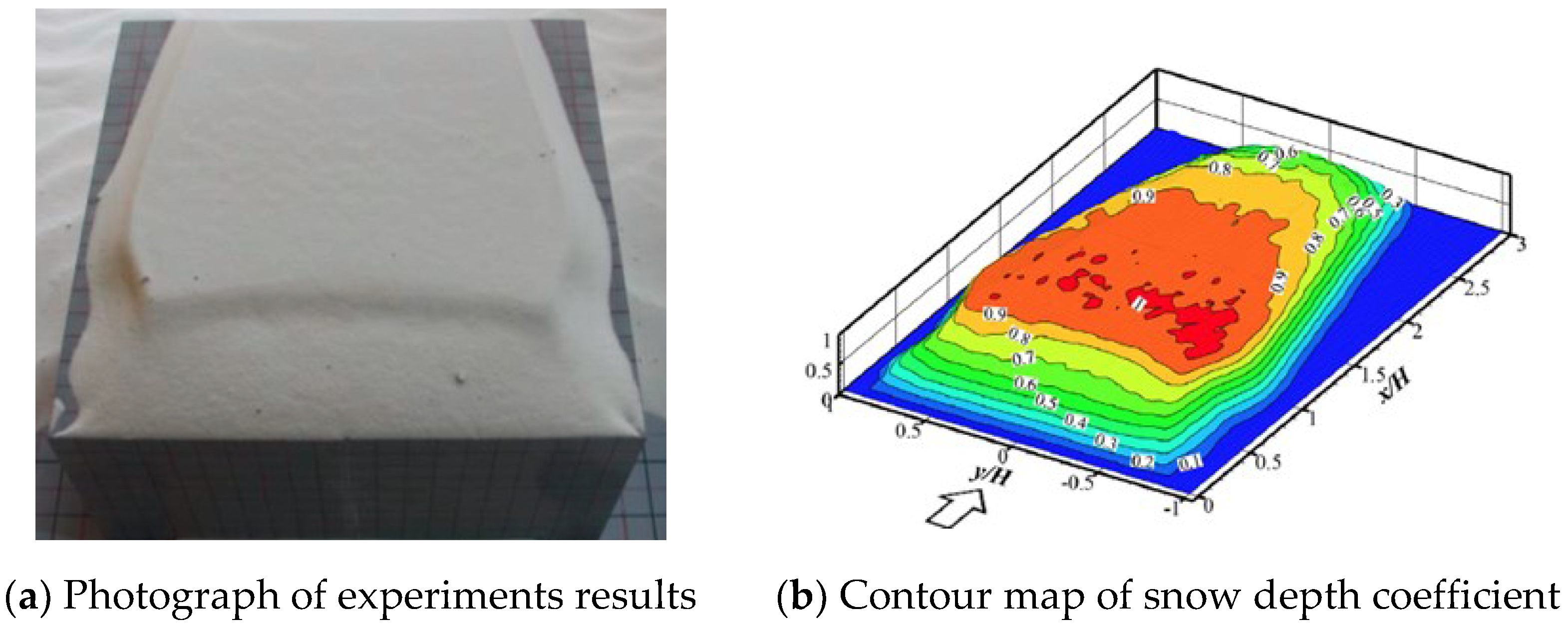
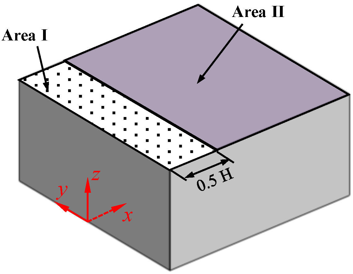
2.1. Geometry Model with Snowdrift

To obtain the snowdrift configuration, the authors conducted wind-blowing snow experiments in a wind tunnel, where high-density silica was used to model the actual snow particles based on a similarity criterion, and low-rise flat-roof buildings with different aspect ratios were considered the research objects. The details of previous wind-blowing snow experiments can be found in the literature [23]. Figure 1 depicts a typical photograph of a model with a snowdrift and the snow depth coefficient. Adopting the oblique photography technique to obtain the point cloud of the snowdrift surfaces, this method is considered to have comparable accuracy to 3D scanning [31,32], and it is easier to use. The geometric model with snowdrift can further be reconstructed from the point cloud. The schematic view of the test model geometry with snowdrift is depicted in Figure 2.

In the present study, the snowdrift model was formed on the flat-roof buildings under the velocity conditions of $U_H=4.5 \mathrm{m}/\mathrm{s}$, as used in previous wind tunnel tests, they were considered to be in a stable form, and different aspect ratios of the low-rise building were considered. In contrast, the building model without snowdrift was used as a control.

Table 1. Model cases.

Model	L/H	W/H	Case Description
Model 1	1	2	No snow (M1_N)
			Snowdrift (M1_S)
Model 2	2	2	No snow (M2_N)
			Snowdrift (M2_S)
Model 3	3	2	No snow (M3_N)
			Snowdrift (M3_S)
Model 4	2	1	No snow (M4_N)
			Snowdrift (M4_S)
Model 5	2	3	No snow (M5_N)
			Snowdrift (M5_S)

provides some descriptions of the model cases. For conciseness of discussion, a notion of ‘M 1_N’ is used to denote the No Snow case for model 1, and so on for all other building models.

2.2. LES Turbulent Model

LES simulated the transient flow by filtering the size of the eddies with the filter width, where the large eddies were directly resolved, and the small eddies were modeled by the sub-grid-scale (SGS) turbulence model. The governing equations for 3D LES with the SGS model are shown as follows:

$$\{\begin{array}{c}\frac{\partial {\overline{u}}_i}{\partial t}+\frac{\partial {\overline{u}}_i{\overline{u}}_j}{\partial x_j}=-\frac{1}{\rho }\frac{\partial \overline{p}}{\partial x_i}+\frac{\partial }{\partial x_j}\left(\nu \frac{\partial {\overline{u}}_i}{\partial x_j}\right)-\frac{\partial {\tau }_{ij}}{\partial x_j}\\ \frac{\partial {\overline{u}}_i}{\partial x_i}=0, \end{array}$$

(1)

where $u_i$ and $u_j$ are the velocity components, and $\rho \mathrm{and} \nu$ are the density and viscosity, respectively. The bar lines indicate the filtering operator, and the incompressible form of the SGS stress term ${\tau }_{ij}$ is defined as:

$${\tau }_{ij}=\overline{u_i{u}_j}-{\overline{u}}_i{\overline{u}}_j.$$

(2)

the SGS stress term is normally used to approximately calculate the following:

$${\tau }_{ij}=-2{\mu }_{SGS}{\overline{S}}_{ij}+\frac{1}{3}{\tau }_{ii}{\delta }_{ij},$$

(3)

where ${\overline{S}}_{ij}$ is the SGS turbulent viscosity, which can be defined as ${\overline{S}}_{ij}=\frac{1}{2}\left(\partial {\overline{u}}_i/\partial {\overline{x}}_j+\partial {\overline{u}}_j/\partial {\overline{x}}_i\right)$. ${\tau }_{ii}$ is the isotropic term that could be simply ignored if the incompressible flow is defined. ${\mu }_{SGS}$ is the SGS eddy viscosity:

$${\mu }_{SGS}=\rho L_S^2\left|\overline{S}\right|=\rho {\left(C_S\mathsf{∆}\right)}^2\sqrt{2{\overline{S}}_{ij}{\overline{S}}_{ij}}$$

(4)

where L_S is the mixing length of the subgrid scales; $C_S$ is the Smagorinsky constant, which changes depending on the type of flow. In the present LES study, to simulate the small eddies, the dynamic Smagorinsky–Lilly (DSL) was selected, and the value of $C_{SGS}$ was computed each time based on the information provided by the resolved scales of motion [33,34].

2.3. Domain Size and Boundary Conditions

This paper used a computational domain size of $42 \mathrm{H}\left(x\right)\times 20 \mathrm{H}\left(y\right)\times 10 \mathrm{H}\left(z\right)$, as shown in Figure 3. The distance from the windward face to the inlet boundary was about 10 H, while 9 H was set from the lateral and top boundary to the model face. The leeward face to the outlet boundary was approximately 30 H. The blockage rate met the relevant requirements, which satisfied the requirements of the relevant CFD guidelines [35,36].

Because of the simple and regular building model, the hexahedral-structured mesh configuration was more suitable for discretizing the computational domain. The schematic view of the grid configuration can be seen in Figure 3. Before the formal LES calculation, a sensitivity test of the grid independence was conducted to obtain a more appropriate mesh size, and detailed information can be found in Section 3.1.

The inlet condition of the numerical simulation was consistent with previous PIV wind tunnel experiments [2] to conveniently verify the validation of the numerical method. The measured profile of the oncoming wind information is shown in Figure 4, where the mean streamwise velocity is fitted by the log law as follows:

$$u\left(z\right)=\frac{u_{ABL}^{*}}{\kappa }\ln \left(\frac{z+z_0}{z_0}\right)$$

(5)

Here, $u_{ABL}^{*}$ is the friction velocity of the ground surface, $\kappa$ is the von Karman constant (0.41), and $z_0$ is the roughness height with a value of 0.00017 m. The turbulent kinetic energy and the dissipation rate were calculated using the following equations:

$$k\left(z\right)=1.5{\left[u\left(z\right)I_u\left(z\right)\right]}^2$$

(6)

$$\epsilon \left(z\right)=C_{\mu }^{3/4}\frac{k{\left(z\right)}^{3/2}}{\kappa z}$$

(7)

where the value of $C_{\mu }$ is 0.09, and $I_u\left(z\right)$ is the turbulence intensity obtained from a wind tunnel.

The vortex method was employed to generate the turbulence fluctuations at the inlet. This method inserts the perturbations into the mean wind velocity profile by randomly generating certain numbers of 2D vortices on the inlet of the computational domain [37], and it has been widely used by many researchers to predict the wind pressure on building surfaces [5,38,39]. For a detailed description of this method, the reader can refer to the literature [37].

As for the remaining boundary conditions, the no-slip wall boundary condition was imposed on the surfaces of the test models and the ground surface. The sides and top of the computational domain were defined as a symmetry boundary condition used to simulate the zero-shear slip walls in viscous flows, and zero static pressure was adopted at the outlet.

2.4. Solution Scheme and Setting Parameters

The parameter settings of the present numerical simulation were similar to the previous research of the author [2]. All of the simulations were performed using Ansys Fluent 2019R1. The pressure–velocity coupling was achieved using the PISO (Pressure-Implicit with Splitting of Operators) algorithm, and the pressure interpolation was solved by the second-order scheme. To avoid any unphysical oscillations in the simulation fields, the bounded central differencing (BCD) scheme was applied to the momentum equations. Meanwhile, the bounded second-order implicit scheme was adopted for the temporal discretization to obtain better stability.

The time step size was set as $\mathsf{∆}t=2.0\times {10}^{-4} \mathrm{s}$, and the mean values of the CFL number did not exceed 0.05. Each LES case was initialized with the solution results from an RANS simulation. After an initialization period of $T_{ini}=2.0 \mathrm{s}$, the data acquisition duration was set as $T_s=7.0 \mathrm{s}$ to ensure that the statistical samples were long enough to obtain converged statistics. The Hewlett-Packard high-performance computer (HPC) facility at Southwest Jiaotong University was used to carry out all of the LES simulations, which employed 128 CPUs for each numerical case.

2.5. Data Sampling and Processing

The wind pressure coefficient $C_{Pi}$ is defined as follows:

$$C_{Pi}=\frac{P_i-P_{ref}}{0.5\times \rho u_{ref}^2}$$

(8)

where $P_i$ is sampling pressure at the i time, $P_{ref}$ is the reference pressure, and $\rho$ is the density of air. Thus, the mean pressure coefficient ${\overline{C}}_P$ can be obtained as follows:

$${\overline{C}}_P=\frac{1}{n}{{\displaystyle \sum }}_{i=0}^n{C}_{Pi}$$

(9)

where n is the total number of sampling times. The fluctuating pressure coefficient $C_P^{\prime }$ is defined as follows:

$$C_P^{\prime }=\sqrt{{\displaystyle \sum }_{i=0}^n\frac{1}{n}{\left(C_{Pi}-{\overline{C}}_P\right)}^2}$$

(10)

3. Sensitivity Analyses and Validation

3.1. Check the Grid Independence

In the present sensitivity analyses, Model 2 without snowdrift was considered to be a reference, and a streamwise mean velocity ($\overline{u}/u_{ref}$) of x/H = 2.5 and the mean pressure (${\overline{C}}_p$) on the roof center (y/H = 0.0) were used as the physical quantities analyzed. Three different refined grids (G1, G2, G3) were tested, and their detailed information is presented in

Table 2. Mesh detail parameters for G1, G2, and G3.

Mesh Type	Grid Numbers on Building Surfaces	The Height of the First Grid on Building Surfaces (m)	Grid Numbers $(\times {10}^4)$	y+ on Building Surfaces
G1	$30\left(x\right)\times 30\left(y\right)\times 27\left(z\right)$	$4\times {10}^{-4}$	70.3	$\approx 10.0$
G2	$41\left(x\right)\times 41\left(y\right)\times 40\left(z\right)$	$4\times {10}^{-5}$	188.6	$\approx 1.0$
G3	$60\left(x\right)\times 60\left(y\right)\times 50\left(z\right)$	$2\times {10}^{-5}$	534.7	$\approx 0.5$

. Figure 5a,b depict the results of the grid resolution tests. As shown in the comparison of the streamwise mean velocity and the mean pressure coefficient, the results of the coarse grid and medium value are quite different, while there is only a relatively small difference between the fine and basic grids. Specifically, for the distribution of the mean wind pressure in the separation–attachment region of the roof, the numerical results between the coarse and medium grid are significantly different. Thus, compared with fine and coarse grids, the medium grid can provide a good compromise.

3.2. Influence of the Sampling Time

The description of turbulence characteristics is usually based on statistical samples, so statistical sampling time is an important parameter affecting the statistical results. The analysis of the sampling time was conducted using the medium grid, and the effects of the different sampling times of 1.0 s, 2.0 s, 3.0 s, 4.0 s, 5.0 s, and 6.0 s on the numerical results were examined, respectively. As shown in Figure 6, taking the results of 6.0 s as a reference, the comparisons of the mean pressure and the fluctuating pressure coefficient on the roof’s central axis under different sampling times are depicted. As one can see, with the increasing sampling time, the statistical value of the wind pressure coefficient tends to stabilize gradually. It indicates that the statistical value of the variables will hardly change after the sampling time exceeds 6.0 s. Therefore, the final statistical sampling time was determined to be 7.0 s in the present LES calculations.

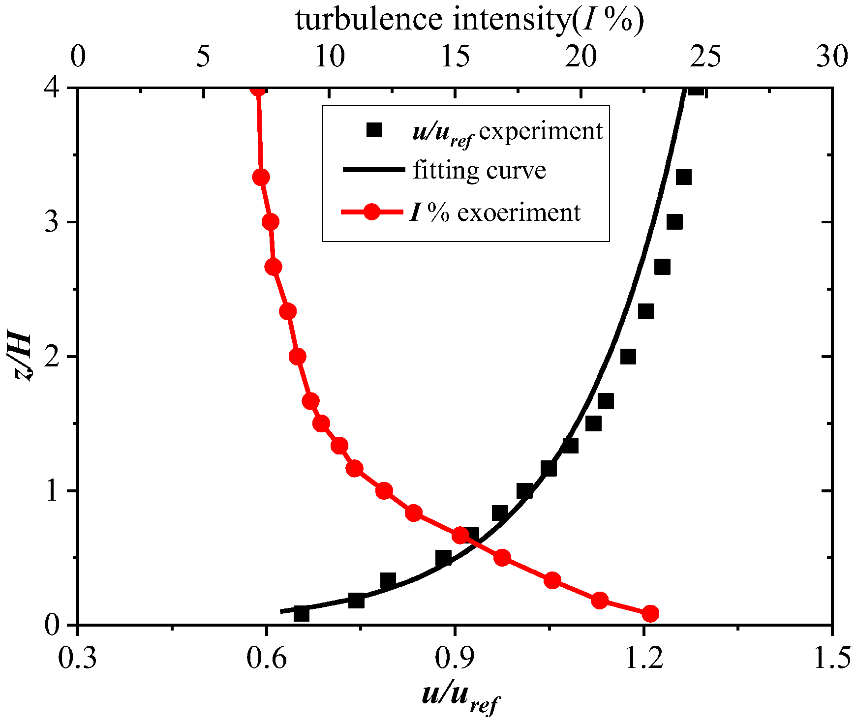
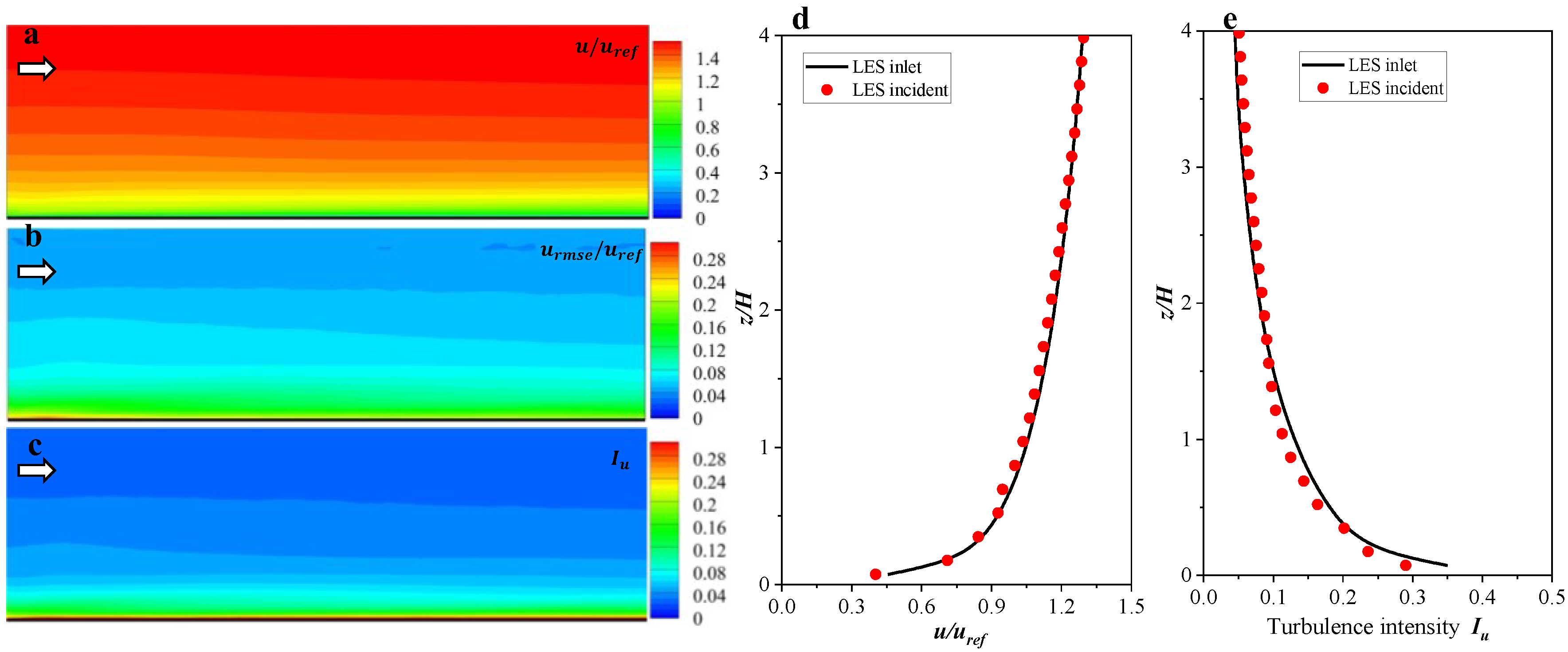
3.3. Self-Preservation Test of the Oncoming Flow

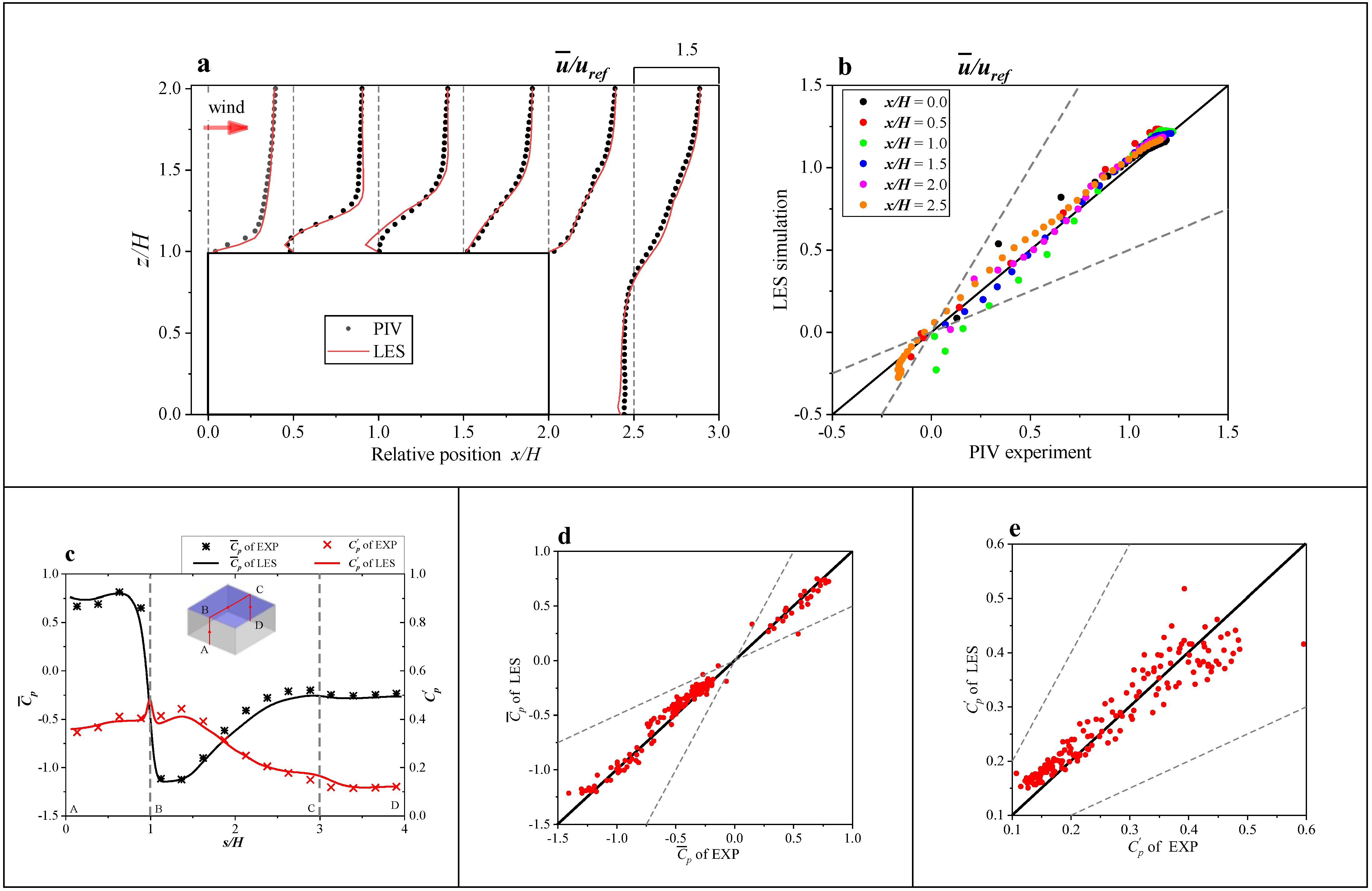
In the present study, testing the self-preservation of the oncoming flow was preferentially conducted in an empty computational domain without a building model, where the domain size, grid configuration, boundary conditions, and solution parameters were consistent with those in Section 2. Based on the calculation results, Figure 7a–c depicts the contour map at the middle planer for $u/u_{ref}$, $u_{rmse}/u_{ref}$, $I_u$. It can be seen that good self-preservation for all of the physical variables can be found in the streamwise direction. Figure 7d,e show a quantitative comparison of the distributions of the variables at the location of the inlet and model incident, a consistency between them can be found by comparing the data distribution. Therefore, in conclusion, the numerical method and the settings of the relevant parameters in the present study can well reproduce the flow field in the wind tunnel test with good self-preservation.

3.4. Validation

In this section, the author uses Model 2 without snowdrift as a reference. Based on the previous wind tunnel experiments, the numerical results were quantitatively analyzed and compared from two aspects, flow velocity ($\overline{u}$) and the roof wind pressure coefficient ($C_p$). The comparison of the flow velocity was based on the previous database carried out by the author in the PIV wind tunnel [2], while the wind pressure coefficient was referenced in the database of Tokyo Polytechnic University [40].

Figure 8a shows that the distribution of the mean streamwise velocity is quantitatively compared at the positions of x/H = 0.0, 0.5, 1.0, 1.5, 2.0, and 2.5, which shows that the numerical results from the LES are consistent with the PIV experiments. Meanwhile, from the quantitative comparison in Figure 8b, it is found that the compared point pairs are almost clustered around the ideal line of a 1:1 relationship. This indicates that the LES method adopted in the present study can accurately predict the mean velocity field. The comparisons of the time-averaged and standard deviation wind pressure are depicted in Figure 8c–e, where the wind tunnel experiments from Tokyo Polytechnic University [36] were used as a validation database. Figure 8c shows the distributions of the wind pressure coefficients along the middle axis of the roof, and Figure 8d,e show the corresponding quantitative comparisons of the time-averaged and STD pressure coefficients between the LES and wind tunnel experiments. As one can see, the results from the presented LES prediction are consistent with the wind tunnel experiments, although the point pairs of the STD pressure coefficient shown in Figure 8e are relatively scattered around the ideal line. This indicates that the numerical settings of the present LES method are suitable for predicting accurate numerical results, and it is well verified by comparing them with the previous wind tunnel experiments.

4. Results and Analyses

4.1. Airflow

When a large amount of snow accumulates on the roof, the original roof shape changes, which leads to significant changes in the flow field near the roof. The following only presents a brief analysis of the streamwise mean velocity and the transient flow evolutions at the xoz planer for a model with or without snowdrift; for more detailed analysis and research, the reader can refer to the previous literature reported by the author [1,2].

4.1.1. Time-Averaged Streamwise Velocity

Figure 9 depicts the distributions of the time-averaged streamwise velocity and streamlines at the xoz planer for some typical models with or without snowdrifts. The red-dotted lines in the contour map represent the separating streamlines, which can be calculated by $\Psi (z)={{\displaystyle \int }}_{wall}^{z}udz=0$. The area enclosed by the separation line and the roof surface can reflect the size of the separation bubble, and the intersection of the separation line and the roof at the rear is the average reattachment point. As shown in Figure 9, it is evident from the figures that the size, both the vertical and streamwise extents, of the mean separation bubble grows monotonically as the windward width increases, which coincides with the findings of previous research [41]. However, the existence of a snowdrift significantly affects the distribution of the velocity field and the shape of the separation bubbles on the roof. As one can see, there is an obvious negative velocity above the roof when there is no snow, and the highest point of the separation line is farther away from the roof; the size of the separation bubble is larger than that of the snowdrift case. However, the negative velocity above the roof almost disappears for snowdrift cases, and the separation bubble becomes smaller and closer to the roof surfaces. Thus, it can be inferred that the snowdrift will accelerate the passing velocity over the building roof.

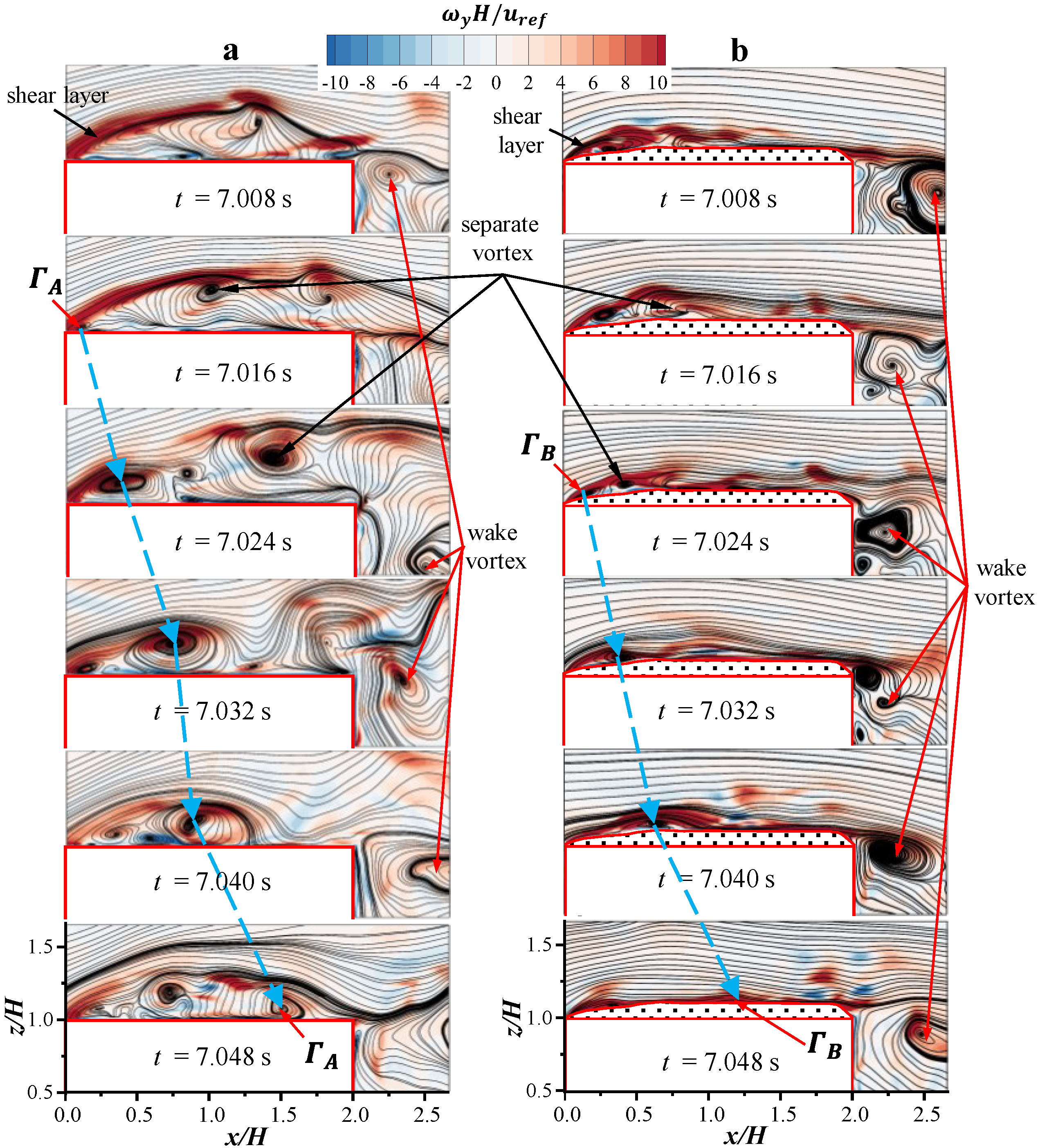
4.1.2. Instantaneous Flow Feature

To better analyze the influence of snowdrifts on the flow field, the direct approach is used to compare the instantaneous flow feature above the roof with or without snowdrifts. In this section, M2 will be taken as a reference, and the instantaneous flow feature at the xoz planer will be compared and analyzed. As shown in Figure 10, the figures depict the instantaneous streamlines and vorticity field of six different instants from t = 7.008 s to t = 7.048 s for the No Snow and Snowdrift model, respectively. In these figures, attention is directed to the flow structures in the separation bubble on the roof. At the front end of the roof, the vorticity has a larger magnitude, which is caused by the formation of the separated shear layer when the oncoming flow flows through the sharp edge of the roof, and the fluid element in the separated shear layer has high shear deformation. Notably, this kind of high-shear flow has significant instability [42]. According to the related turbulence theory, the high-shear effect of fluid is the internal factor of the transition from laminar flow to turbulence flow, which provides the energy source for vortex generation. Thus, a series of vortices are formed in the separated shear layer, then travel and grow up on the roof, and finally slowly dissipate in the flow field. However, the snowdrift on the roof results in a remarkable difference in the vortices’ movement. When there is no snow on the roof, take vortex ${\Gamma }_A$ as an example for analysis. At t = 7.016 s, vortex ${\Gamma }_A$ is detached from the leading edge of the roof. From t = 7.06 s to t = 7.032 s, vortex ${\Gamma }_A$ is stretched and convected downstream along the building roof. During this process, the high shear–strain fluid in the shear layer continuously provides the energy for the generation of vortices, and the generation of turbulence energy is much larger than that of dissipation. Meanwhile, the merging of several neighboring vortices in the separation bubble can also be observed; thus, the size of vortex ${\Gamma }_A$ on the roof will gradually increase. From t = 7.032 s to t = 7.048 s, the large vortex transforms into a small vortex in this process, and the scales of the vortices decrease gradually. The vortex moves from the farthest position of the vortex core of the roof to reattaching to the roof and is finally dissipated in the wake behind the roof.

When there is a snowdrift on the roof, some differences can be clarified. Taking vortex ${\Gamma }_B$ for analysis, it is seen that the scale of vortex ${\Gamma }_B$ decreases obviously, and the core of the vortex is almost closer to the roof surface during the process of traveling. The main reason is that the narrow space for recirculation on the roof due to the existence of snowdrift results in the shear layer being closer to the roof surface. Furthermore, the vortex generated in the shear layer is more easily affected by the wall friction, so the vortex is quickly dissipated on the roof without an obvious growing-up process of the vortex scale. Compared with the distribution of the time-averaged streamlines in Section 4.1.1, the separation bubble on the building roof can be considered the average trajectories of a series of separated vortices. Therefore, when the size of the separated vortex is significantly suppressed by the snowdrift, the size of the separated bubble is also significantly reduced. Notably, the pressures on the building surface result from the “footprints” of the local flow structures, the variation in the flow field will inevitably lead to the distributed difference of wind pressure on roofs. These issues will be discussed and analyzed in the subsequent sections.

4.2. Wind Pressure Coefficient on Roof

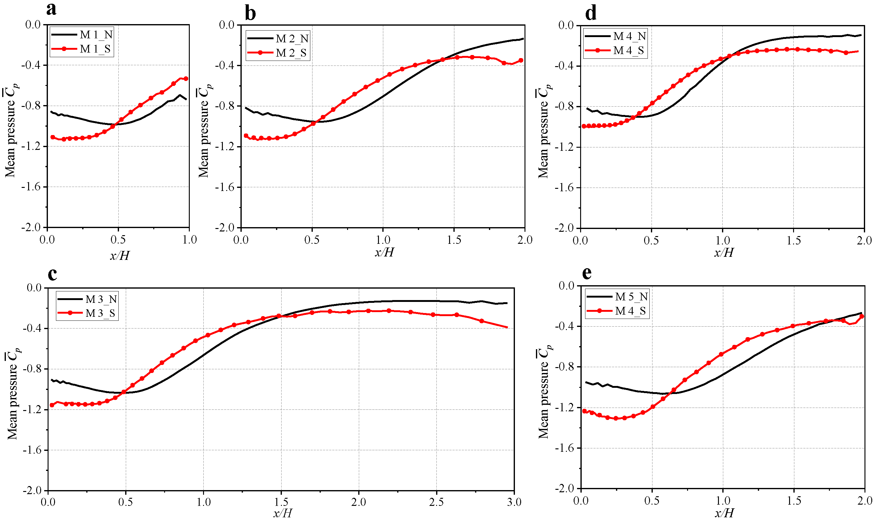
4.2.1. Time-Averaged and Standard Deviation Pressure Coefficient on Roof

Figure 11 quantitatively analyses the time-average (mean) wind pressure coefficient on the middle axis of the No Snow or Snowdrift roofs. When there is no snow, a larger magnitude of negative pressure will occur in the separation region of the roof, and the value of the mean pressure coefficient is around -1 and has no obvious variation. Then the mean pressure increases rapidly along the roof and tends to be stable at the back of the roof. The variation in the mean pressure coefficient with x/H shows a typical ‘S’ curve. When there is a snowdrift on the roof, the ‘S’ curves of the mean pressure coefficient can also be observed. However, some obvious differences between them should be clarified. As shown in the comparisons in Figure 11, it is found that the magnitude of negative pressure in the separation region of the snowdrift roof will be significantly amplified. The comparisons of the standard deviation (STD) wind pressure are shown in Figure 12; the distribution of the STD pressure coefficient along the roof axis has a tendency to increase first and then decrease regardless of whether there is snowdrift or not on the roof. However, the snowdrift will change the position of the peak value of the STD wind pressure. As shown in Figure 12, the peak values of the STD pressure for all of the models without snowdrifts are almost around 0.3, and the corresponding positions are in the region of 0.5 < x/H < 1.0. When there is a snowdrift, the peak values of the STD wind pressure will increase to around 0.35. Meanwhile, the corresponding positions of the peak value will also increase compared with No Snow, and most of them are in the region of x/H < 0.5.

From the analyses compared with the airflow characteristics in Section 4.1, the reason can be deduced as follows: when there is no snow, a typical and large-scale separation bubble will form on the roof after the oncoming flow separates from the leading edge of the roof, and the vortex core will be far away from the separation point and the roof surface. Thus, the mean wind pressure in the windward region for the No Snow roof is smaller than that of a Snowdrift. However, the snowdrift causes the separation shear layer to be closer to the roof surface, and the recircle space is reduced; thus, the reattachment effect is weakened. As a result, the size of the separated vortex is significantly reduced, and its position is earlier and closer to the model surface. Therefore, in the region of x/H < 0.5, the separated vortex closer to the snowdrift roof surface will result in a larger magnitude of the time-averaged and STD wind pressure coefficient. In the region of x/H > 0.7, the large-scale separated vortices formed on the No Snow roof slowly dissipate, and it has a greater impact on the STD wind pressure. However, the small-scale vortices formed on the Snowdrift roof will be more easily dissipated due to the wall friction, so the corresponding STD pressure coefficient for the Snowdrift roof will also be reduced.

4.2.2. Area-Averaged Pressure Coefficient in the Windward Region

As shown above section, the snowdrift on the roof will cause an obvious difference in wind pressure, especially in the windward region of the roof. Thus, the area-averaged pressure coefficient in the windward region will be discussed in this section. Figure 13 depicts the schematic diagram of the roof division, where Area I denotes the windward region with a range of 0 < x/H < 0.5, and Area II denotes the non-windward region with a range of x/H > 0.5. Here attention is directed to the area-averaged pressure coefficient in the windward region, and the analysis variables include the area-averaged value of the mean, standard, and minimum pressure coefficient in the windward region. Taking variable $\phi$ as an example, the area-averaged value of $\phi$ can be expressed as follows:

$${\phi }_{\_Aa}=\frac{{{\displaystyle \sum }}_{i=1}^m{\phi }_i\times A_i}{A_{tol}}$$

(11)

where, ${\phi }_i$ is the center value of the ith element in a roof surface, $A_i$ is the weighted area of the element, $A_{tol}$ is the total area of this surface.

To obtain the minimum value of the pressure coefficient, the peak gust factor method [43] was used based on the time-averaged and standard pressure coefficient, which can be defined as follows:

$$C_{p, min}={\overline{C}}_p-g_{NG}{C}_p^{\prime }$$

(12)

where, $g_{NG}$ denotes the peak gust factor, and in the present study, $g_{NG}=8$ was selected. As shown in Figure 14, the comparison of the area-averaged value of the wind pressure coefficient for roofs with or without snowdrift is depicted. It can be seen that the magnitude of the Snowdrift cases is significantly larger than that of No Snow cases. Taking the area-averaged standard pressure coefficient as an example for analysis (Figure 14b), the values of all models are less than 0.3 without snow, and greater than 0.3 with snow, even more than 0.35 for M5. To quantitatively describe the effect of snowdrift on the area-averaged pressure coefficient, Relative Difference (RD) was introduced:

$$RD=\frac{{\left({\phi }_{\_Aa}\right)}_S-{\left({\phi }_{\_Aa}\right)}_N}{{\left({\phi }_{\_Aa}\right)}_N}\times 100\%$$

(13)

where, ${\phi }_{\_Aa}$ denotes the area-averaged value of variable $\phi$, and the subscripts N and S indicate the No Snow and Snowdrift cases, respectively.

The comparisons of the RD values for all models’ area-averaged pressure coefficients are depicted in Figure 14d. It can be seen that the snowdrift has the most significant effect on the increase in the standard wind pressure in the windward region, with an increasing ratio of more than 20%, and even 40% for model M5. The influence on the time-average wind pressure is small, and the increasing ratio is between 15% and 30%. Therefore, combined with the analyses above, it seems that the wind loads on the windward region of the roof have larger values.

4.3. Probability Density and Energy Spectrum of Fluctuating Pressure

The probability density function (PDF) reflects the random characteristics of the fluctuating wind pressure and tests whether it has the features of a Gaussian distribution. The power spectrum distribution (PSD) describes the characteristics of the fluctuating wind pressure in the frequency domain. In the present section, the author uses M3 as the reference object and sets the wind pressure monitoring points at eight locations (x/H = 0.01, 0.25, 0.50, 0.75, 1.00, 1.50, 2.00, and 2.50) on the central axis of the roof with or without snow and the wind pressure time history data are obtained (Figure 15). On this basis, the influence of snowdrift on the probability density function and the power spectrum of the fluctuating pressure is analyzed.

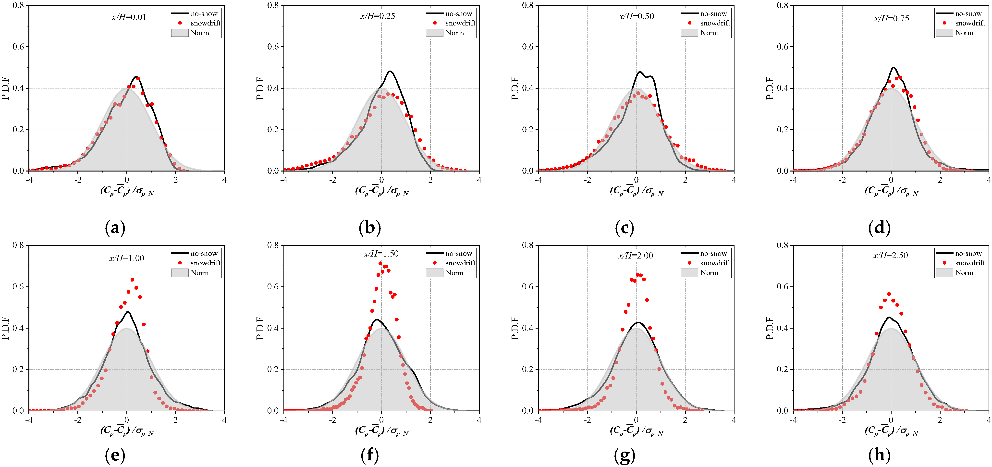
4.3.1. Distribution of Probability Density Function

Figure 16 depicts the PDF of the fluctuating pressure coefficient at the different monitoring points, where the abscissa is the dimensionless fluctuating wind pressure coefficient. ${\sigma }_{p_N}$ denotes the standard deviation of the fluctuating wind pressure coefficient at the monitoring point without a snowdrift, and the grey filling part represents the standard normal distribution (or Standard Gaussian distribution). For the convenience of subsequent analysis, the interval of $\left(C_p-{\overline{C}}_p\right)/{\sigma }_{p_N}\in \left[-1,1\right]$ is defined as the low-fluctuation range of the fluctuating wind pressure, and the intervals of $\left(C_p-{\overline{C}}_p\right)/{\sigma }_{p_N}$ < −2 and $\left(C_p-{\overline{C}}_p\right)/{\sigma }_{p_N}$ > 2 are defined as the negative and positive high-fluctuation ranges, respectively.

At the monitoring point of x/H = 0.01 near the leading edge, the PDF curves with or without snowdrift are the same. The reason is that the fluctuating wind pressure at the separation point is mainly controlled by the unstable flow in the shear layer, and the snowdrift has little effect on it. At the locations of x/H = 0.25 and 0.5 in the windward region, the PDF curves for no snow or snowdrift cases are different. As one can see that in the low-fluctuation range, the relative probability of a no snow case is larger than that of a Snowdrift case. While the high-fluctuation range is just the opposite, which indicates the high amplitude energy of the fluctuating wind pressure accounts for a larger proportion when there is snowdrift. According to the results from Section 4.1 and Section 4.2, it is inferred that the fluctuating wind pressure in the windward region will be simultaneously affected by the unsteady flow of the shear layer and the separated vortex convected downstream along the roof. When there is a snowdrift on the roof, the scale of the separated vortex will be significantly strained, and the vortex core will be much closer to the roof surface. Thus, under the action of the vortex core being closer to the roof surface, the fluctuating wind pressure is also larger. At the location of x/H = 0.75, it can be seen from Figure 16d that the fluctuating pressure coefficients on the roof with or without snowdrift are almost the same, thus the corresponding distributions of PDF also coincide. As for the monitoring points in the region of x/H > 0.75, the peak values of the PDF for the Snowdrift case are larger than that of the No Snow case, which means the energy of the fluctuating wind pressure for the Snowdrift case is more concentrated in the low-fluctuation range. Meanwhile, the values of the PDF for Snowdrift cases in the high-fluctuation range are smaller than that of the No Snow cases. Combined with the flow field in Section 4.1, the reason is that a large-scale vortex will form on the building’s roof when the oncoming flow is separated at the leading edge of the No Snow roof, and the large-scale vortex with larger turbulence energy will undergo a long traveling process on the roof, and gradually dissipate in the wake. However, the small-scale vortex formed on the Snowdrift roof is closer to the roof surface and more easily dissipated under the combined action of the wall friction and fluid viscosity.

Additionally, compared with the Standard Gaussian distribution, the peak values of the PDF curves for the fluctuating wind pressure in the windward region (x/H < 0.5) are distributed on the right side of the zero point, which means that the fluctuating wind pressure has non-Gaussian distribution characteristics of negative skewness. As the monitoring points move to the back of the roof, the peak values of the PDF curves gradually approach the zero point, which indicates that the fluctuating wind pressure in these areas is more consistent with the Gaussian distribution. Furthermore, in the region where the fluctuating wind pressure obeys the non-Gaussian distribution, the fluctuating wind pressure mainly fluctuates in the negative direction, which means a larger peak gust factor occurs in the windward region and results in a larger magnitude of local wind pressure.

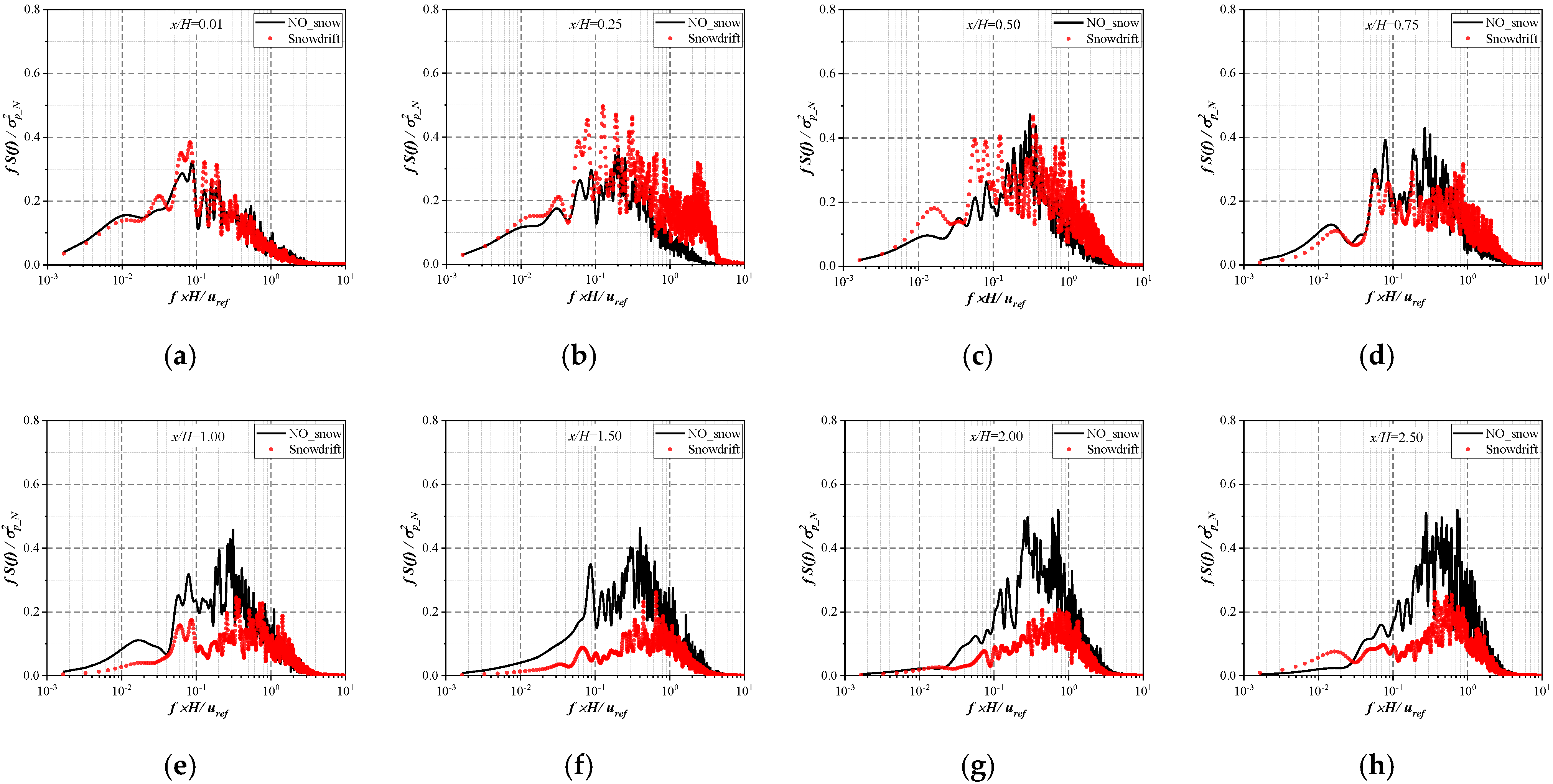
4.3.2. Frequency Domain Features

The power spectrum of the fluctuating wind pressure can be obtained using a Fourier transformation of the time history data to analyze the influence of snowdrift on the energy distribution of the fluctuating wind pressure in the frequency domain. Figure 17 depicts the PSD of the fluctuating pressure at different monitoring points on the roof, where f denotes the frequency and ${\sigma }_{p_N}^2$ represents the variance of fluctuating pressure at the monitoring point without snowdrift. At the point of x/H = 0.01 near the leading edge, the predominant frequency corresponding to the peak values of PSD of the fluctuating wind pressure are all located in the low-frequency range ($fH/u_{ref}<0.1$). The low-frequency fluctuation is mainly caused by the K-H instability in the high-shear flow near the leading edge of the roof [42]. Meanwhile, the K-H instability in the shear layer will transfer turbulence energy to the flow field by the intermittent ‘flapping motion’, thus inducing vortex generation [44]. As the airflow goes downstream in the separating shear layer, the vortex energy is continuously accumulated, and the spectral peak values of the fluctuating wind pressure will tend to increase. Meanwhile, the predominant frequency of each monitoring point also increases gradually. This is because the large-scale vortices formed in the shear layer will transform into small-scale vortices in the traveling process, which causes the vortex energy to transform from low frequency to high frequency.

Snowdrift has a significant effect on the power spectrum of the fluctuating wind pressure. As one can see that in the windward region of the roof, the spectral values of the fluctuating wind pressure for the Snowdrift case are larger than that of the No Snow case, especially in the high-frequency range. The main reason is that the snowdrift accelerates the velocity field near the roof and effectively suppresses the scale of separated vortices, and small vortices will be formed, convected, and dissipated downstream at a faster frequency. Therefore, the fluctuating wind pressure energy for the snowdrift cases will be more concentrated in high-frequency intervals. With the vortex traveling downstream along the roof, the large-scale vortex formed on the no-snow roof is far away from the roof and is dissipated slowly. While the small-scale vortex generated on snowdrift roof is more easily dissipated under the wall friction. Thus, at the back of the roof, the fluctuating wind pressure energy for the Snowdrift case is smaller than that of the No Snow case.

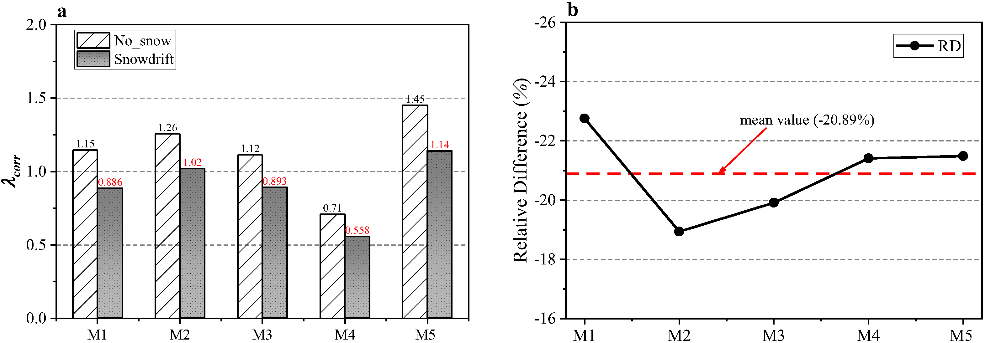
4.4. Cross-Correlation Analysis

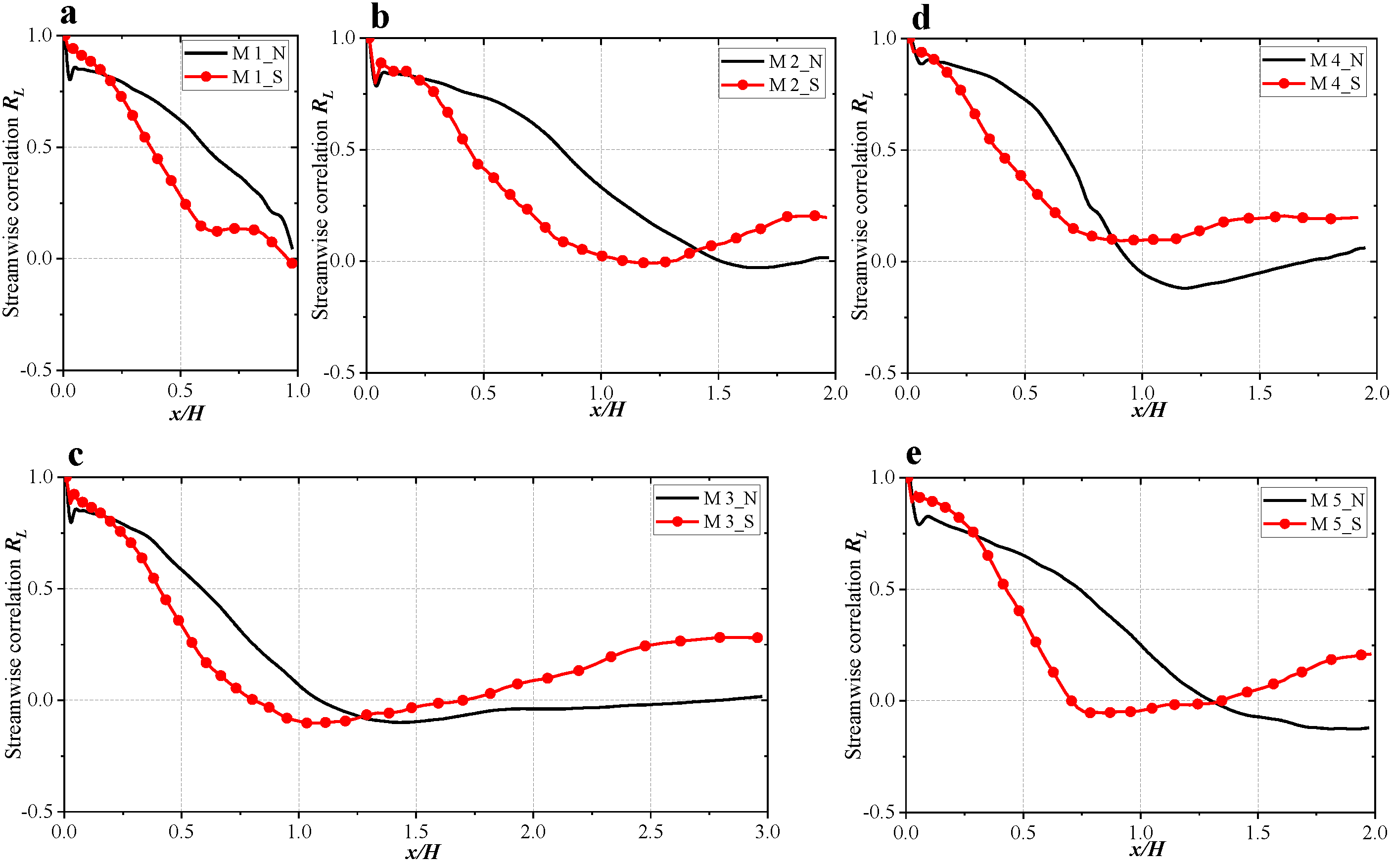
4.4.1. Streamwise Correlation

After separating from the leading edge of the roof, a typical separating vortex is formed. Due to the influence of the vortex, the fluctuating wind pressure acting on the roof has a strong cross-correlation. The streamwise correlation of the fluctuating wind pressure can be described by $R_L$, which is expressed as:

$$R_L=\frac{\overline{C_p\left(t,x\right)C_p\left(t,x_0\right)}}{C_P^{\prime }\left(x\right)C_p^{\prime }\left(x_0\right)}$$

(14)

where $C_p\left(t,x\right)$ is the fluctuating wind pressure at the location of x, and $C_p\left(t,x_0\right)$ denotes the fluctuating wind pressure at the reference point $x_0\left(x_0=0.02H\right)$. The over-bar denotes a time-averaged quantity. $C_P^{\prime }\left(x\right)$ and $C_p^{\prime }\left(x_0\right)$ are the standard deviations of the corresponding fluctuating wind pressure. As shown in Figure 18, the streamwise correlation coefficient decreases rapidly with the increase of x/H. However, the snowdrift has an important effect on the streamwise correlation, when there is a snowdrift on the roof, the $R_L$ tends to decrease faster downstream along the building roof. Thus, the location of the minimum value of $R_L$ will be significantly advanced.

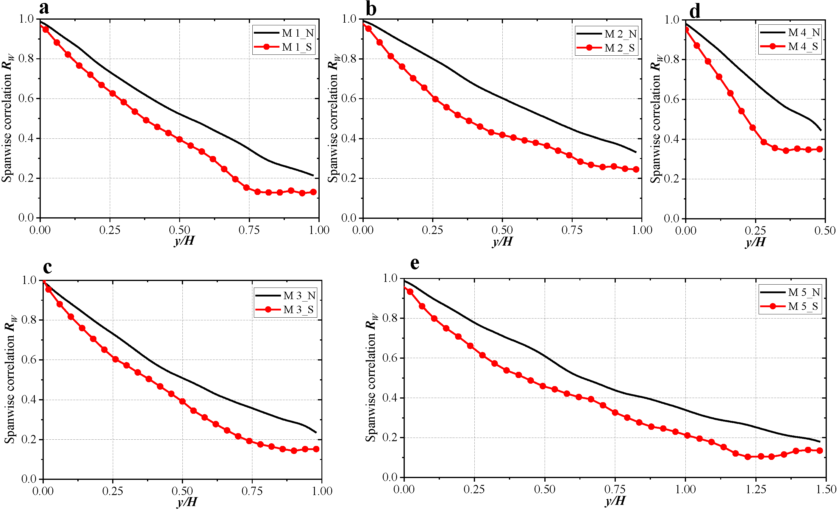
4.4.2. Spanwise Correlation

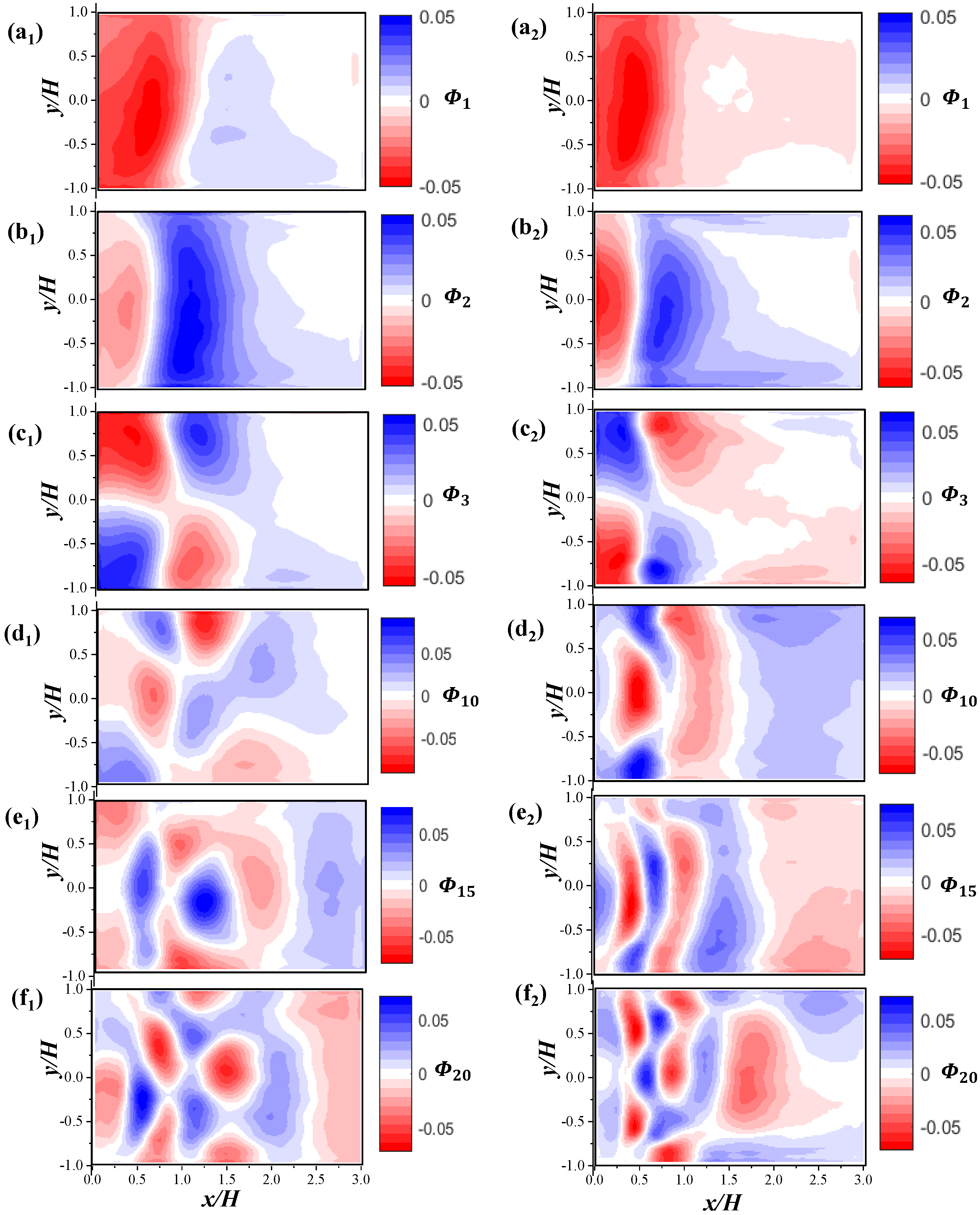
The cross-correlation of the fluctuating wind pressure induced by the separation bubble is not only reflected in the streamwise direction but also in the spanwise direction. The spanwise distributions of the unsteady pressures reflect the three-dimensional characteristics and are of vital importance in calculating the global forces. The spanwise correlation, $R_W$,which is similar to the streamwise correlation $R_L$, can be defined as follows:

$$R_W=\frac{\overline{C_p\left(t,y\right)C_p\left(t,y_0\right)}}{C_P^{\prime }\left(y\right)C_p^{\prime }\left(y_0\right)}$$

(15)

where the point $y_0$ at x/H = 0.5, y/H = 0.0 will be considered as reference, and the spanwise correlations of other monitoring points at the line of x/H = 0.5, 0.0 < y/H < W/2 are obtained. As shown in Figure 19, the spanwise correlation $R_W$ decreases rapidly as the y/H increases. When there is no snow on the roof, the attenuation curve of the spanwise correlation coefficient with the y/H almost satisfies the linear correlation, which indicates the decay rate of the spanwise correlation coefficient is almost the same induced by the separation bubble is almost the constant, and the spanwise integral scale also remains almost unchanged. However, when there is a snowdrift on the roof, the attenuation curve of the spanwise correlation coefficient of the fluctuating wind pressure is nonlinear, and the decay rate is also significantly faster than that of a no-snow roof. To quantify the effect of snowdrift on the spanwise correlation of fluctuating pressure, according to the suggestion of Saathoff and Melbourne [45], the integral length scale of spanwise correlation ${\lambda }_{corr}$ is introduced:

$${\lambda }_{corr}=\frac{2}{H}{{\displaystyle \int }}_0^l{R}_W dy$$

(16)

where l denotes the distance from the reference point to the side of the roof, and the value is the half-width of the roof (W/2). Meanwhile, the integral length scale is normalized by the reference height H.

In Figure 20, the comparisons of the integral length scale of a spanwise correlation (${\lambda }_{corr}$) for different models are presented. It is shown that the integral scale for the No Snow case is remarkably larger than that of the Snowdrift case. Compared with the airflow characteristics above the roof, the reason can be deduced that the snowdrift significantly restrains the scale of the separated vortex, and the small-scale vortex formed on the snowdrift roof can cause the energy of the fluctuating wind pressure to concentrate in the high-frequency range. However, the fluctuating wind pressure with small-scale and high-frequency characteristics is not conducive to lateral transmission, so the corresponding integral length scale is also reduced. Furthermore, as shown in Figure 20b, it is estimated that the average reduction of the integral length scale of spanwise correlation caused by the snowdrift is about 20%.

4.5. POD Analysis

The wind pressure on a building roof is a complicated random field, and proper orthogonal decomposition (POD) is a powerful method that has been extensively used by many researchers [46,47] to reveal the characteristics of wind pressure on a roof. By adopting suitable and mutually orthogonal eigenfunctions Φ(x, y), the complicated fluctuating wind pressure on the roof can be decomposed into the independent time and space database. It is beneficial for uncovering the most significant structures dominating the pressure field in the space and frequency domains. The POD analyses in the present study are applied to the pressure data on the building roofs with or without snowdrift; only the fluctuating components are included, while the time–mean values are removed. Next, the space covariance is calculated by Equation (17), where i and j denote two measuring points.

$${\widehat{R}}_p\left(x_i,y,x_j,y\right)=p\left(x_i,y,t\right)p\left(x_j,y_j,t\right)$$

(17)

A set of eigenvectors ${\Phi }_n\left(x,y\right)$ and the corresponding eigenvalue ${\lambda }_n$, are introduced to represent the energy contained by each mode, where n denotes the mode’s order. The POD modes ${\Phi }_n\left(x,y\right)$ are evaluated by solving the maximum of the projection of $p\left(x,y,t\right)$. Thus, the matrix composed of eigenvectors is the obtained POD modes and the eigenvalue ${\lambda }_n$ denotes the energy contribution of each POD model. The derivation can be expressed as follow:

$${\widehat{R}}_p\Phi =\lambda \Phi$$

(18)

after the eigenvectors are orthogonalized, the fluctuating pressure field can be expressed as the linear superposition of the principal coordinate and the spatial mode.

$$p\left(x,y,t\right)={\displaystyle \sum }_{m=1}^n{\delta }_m\left(t\right){\Phi }_m\left(x,y\right)$$

(19)

where ${\delta }_m\left(t\right)$ is the principal coordinate, which denotes the expansion coefficients of each POD mode, and the energy contribution of each mode is defined as the proportion of corresponding eigenvalues in all POD modes.

The contribution of the typical POD modes to the total fluctuating energy is shown in

Table 3. Proportion and cumulative proportion of the energy level corresponds to the POD modes.

Description of Building Models		The Proportion of Modes (%)						The Total Proportion of the First 20 Modes (%)
		1st	2nd	3rd	10th	15th	20th
M1	N	31.50	15.58	11.62	1.36	0.75	0.45	88.51
	S	29.66	10.94	9.61	1.70	0.91	0.60	82.07
M2	N	22.59	16.60	8.88	2.08	1.02	0.67	83.75
	S	26.74	9.66	5.98	1.61	1.06	0.70	72.84
M3	N	19.12	14.16	7.16	1.93	1.14	0.76	75.02
	S	20.59	9.97	7.55	1.80	1.14	0.73	70.65
M4	N	30.12	12.75	7.66	1.70	1.02	0.65	83.00
	S	29.12	10.03	8.10	1.73	0.91	0.64	80.33
M5	N	19.70	13.30	8.15	1.82	1.09	0.72	74.03
	S	21.24	10.76	7.18	1.67	1.11	0.74	70.02

for building roofs with or without snowdrifts. The cumulative proportions of the first 20 modes are also depicted for comparison. With the increase in the number of the POD modes, the energy contribution of each mode decreases quickly. Taking the building model of M3_N as an example for analysis, the contributions of the lower order Modes 1, 2, and 3 are 19.12%, 14.16%, and 7.16%, respectively. While the contributions for the higher order Modes 10, 15, and 20 are, respectively, 1.93%, 1.14%, and 0.76%. The contributions for other higher order Modes exceeding 20 are smaller than 1%. This indicates that the larger the order of POD modes, the smaller the energy contributions of the corresponding modes. In other words, these higher modes contain a negligibly small amount of energy. As shown in the comparisons of cumulative proportions, the sum energy proportions of the first 20 modes for all building models are all more than 70%, and the maximum value even reaches 88%. It can be inferred that the fluctuating wind pressure energy is more concentrated in the lower-order modes. Furthermore, comparing the cumulative energy proportions of the first 20 modes between the no snow and snowdrift case, it is found that the cumulative energy proportions for no snow cases are larger than that of snowdrift cases, which indicates that the fluctuating energy in lower order modes for no snow cases is more concentrated than snowdrift cases.

To uncover the most significant structures of the pressure field, the pressure contour maps of typical POD modes are analyzed in the present section. For convenience, the building model M3 will be taken as an example. As shown in Figure 21, it can be found that the distributions of the mode eigenvectors for No Snow and Snowdrift have some considerable similarities in the first three POD modes, the numbers of the peak values of the mode eigenvectors are less, and their locations are mainly distributed in the front half of the roof. While for the high order modes (10th, 15th, and 20th), there are some differences, the numbers of the peak values of the mode eigenvectors significantly increase, and the distributions are more dispersed on building roofs. Additionally, as for the first and second modes, the eigenvectors are symmetrically distributed, with y/H = 0 of the roofs as the axis of symmetry. As the mode orders increase, the eigenvectors develop complicated 3D features. The main reason is that the low-order POD modes are dominated by low-frequency vortices with large turbulence scales, and the high-order modes are controlled by the local small-scale vortices, which have a larger shedding frequency. Additionally, from the comparison of the eigenvectors distribution, it can be found that the extremum values of the eigenvectors for snowdrift cases are more distributed at the leading edge of the roof than for the No Snow cases, which indicates the fluctuating energy on the snowdrift roof is more concentrated in the front region of the roof. It can be deduced by combining the airflow characteristics in Section 4.1 that the snowdrift significantly restrains the scale of the separated vortices, which causes the main vortex of the separation bubble to be located forward and closer to the building surface.

5. Conclusions

In this study, the effect of snowdrift on the airflow and wind pressure around an isolated low-rise flat-roof building was analyzed via a validated Computational Fluid Dynamics (CFD) model based on the Large-Eddy simulation (LES) method. Some summaries and conclusions are delineated below.

According to the sensitivity analyses, it is better to adopt the medium grid configuration and a sampling time of $7.0\mathrm{s}$ to obtain sufficiently accurate numerical results in the present LES studies. Meanwhile, the numerical results of the present LES method are well verified by comparison with previous wind tunnel experiments.

The snowdrift leads to a narrow space for recirculation on the roof and can effectively restrain the size of separation bubbles in the separating–reattachment flow field, which leads to the smaller-scale separated vortices formed on the roof, and they are more easily dissipated under the action of wall friction. Therefore, the snowdrift has a remarkable acceleration effect on the flow field near the building roof.

Due to the small-scale separated vortices formed on snowdrift roofs, the vortex core is significantly forward and closer to the roof surface. Thus, the magnitude of the wind pressure coefficient in the windward region for a Snowdrift roof is larger than that of a no snow roof. Especially for the area-averaged value of the fluctuating wind pressure, the maximum value of the Relative Difference even reaches 40%. Furthermore, through the analysis of time- or frequency domain, cross-correlation, and POD for fluctuating pressure, it is indicated that the snowdrift can cause the fluctuating wind energy to concentrate in the region near the windward side. Thus, to some extent, the formation of snowdrifts on the roof may lead to greater local wind loads, which may be a new challenge for the safety of structures.

6. Discussion and Limitation

In the present article, the author used a low-rise flat-roof building as the research object and quantitatively evaluated the influence of wind-induced snowdrift on the wind loading on the roof using LES calculation. From the research results, the formation of snowdrifts on roofs may lead to greater local wind loads to some extent, especially in the windward area. It may create a new challenge for the safety of building structures. Therefore, these research conclusions have certain reference values for the load design of low-rise flat-roof structures in high-latitude snowy and windy regions. Although there is no direct evidence that the change of wind load caused by snowdrift will cause damage to the roof structure in the investigation of snow disasters, its effect on the roof structure is still unknown. Therefore, the author wants to convey that when we pay more attention to the wind-induced uneven snow load on the roof, it is necessary to consider the change of wind loading due to snowdrift; based on this, we conducted the research work of this paper.

However, the factors considered in the present study are still limited, and the snowdrifts shape on flat roofs with different aspect ratios is given. In nature, the snowdrift shape on the roof will change with the wind speed, roof geometry, wind direction, drifting duration, and the interference of surrounding buildings, which will also lead to a different influence on the wind loads on the roof. Therefore, a lot of research work on this issue is still needed to obtain more applicable results and to improve the relevant codes and standards to guide the load design in actual projects.

References

1. Zhu, F.; Yu, Z.; Liu, Z.; Chen, X.; Cao, R.; Qin, H. Experimental study on the air flow around an isolated stepped flat roof building: Influence of snow cover on flow fields. J. Wind. Eng. Ind. Aerodyn. 2020, 203. [Google Scholar] [CrossRef]
2. Liu, Z.; Yu, Z.; Chen, X.; Cao, R.; Chen, Y. Numerical and experimental studies on the airflow around the low-rise flat-roof buildings with different stable snowdrifts. Cold Reg. Sci. Technol. 2021, 187, 103294. [Google Scholar] [CrossRef]
3. Tominaga, Y.; Akabayashi, S.-I.; Kitahara, T.; Arinami, Y. Air flow around isolated gable-roof buildings with different roof pitches: Wind tunnel experiments and CFD simulations. Build. Environ. 2015, 84, 204–213. [Google Scholar] [CrossRef]
4. Ozmen, Y.; Baydar, E.; van Beeck, J.P.A.J. Wind flow over the low-rise building models with gabled roofs having different pitch angles. Build. Environ. 2016, 95, 63–74. [Google Scholar] [CrossRef]
5. Xing, F.; Mohotti, D.; Chauhan, K. Study on localised wind pressure development in gable roof buildings having different roof pitches with experiments, RANS and LES simulation models. Build. Environ. 2018, 143, 240–257. [Google Scholar] [CrossRef]
6. Mahmood, M. Experiments to study turbulence and flow past a low-rise building at oblique incidence. J. Wind. Eng. Ind. Aerodyn. 2011, 99, 560–572. [Google Scholar] [CrossRef]
7. Dong, X.; Ding, J. Wind pressure characteristics on flat roofs with rounded leading edge. J. Build. Struct. 2019, 40, 28–40. [Google Scholar]
8. Stathopoulos, T.; Zisis, I.; Xypnitou, E. Local and overall wind pressure and force coefficients for solar panels. J. Wind. Eng. Ind. Aerodyn. 2014, 125, 195–206. [Google Scholar] [CrossRef]
9. Jubayer, C.M.; Hangan, H. Numerical simulation of wind effects on a stand-alone ground mounted photovoltaic (PV) system. J. Wind. Eng. Ind. Aerodyn. 2014, 134, 56–64. [Google Scholar] [CrossRef]
10. Wang, J.; van Phuc, P.; Yang, Q.; Tamura, Y. LES study of wind pressure and flow characteristics of flat-roof-mounted solar arrays. J. Wind. Eng. Ind. Aerodyn. 2020, 198, 104096. [Google Scholar] [CrossRef]
11. Akon, A.F.; Kopp, G.A. Mean pressure distributions and reattachment lengths for roof-separation bubbles on low-rise buildings. J. Wind. Eng. Ind. Aerodyn. 2016, 155, 115–125. [Google Scholar] [CrossRef]
12. Akon, A.F.; Kopp, G.A. Turbulence structure and similarity in the separated flow above a low building in the atmospheric boundary layer. J. Wind. Eng. Ind. Aerodyn. 2018, 182, 87–100. [Google Scholar] [CrossRef]
13. Ahmad, S.; Kumar, K. Interference effects on wind loads on low-rise hip roof buildings. Eng. Struct. 2001, 23, 1577–1589. [Google Scholar] [CrossRef]
14. Kim, Y.C.; Yoshida, A.; Tamura, Y. Characteristics of surface wind pressures on low-rise building located among large group of surrounding buildings. Eng. Struct. 2012, 35, 18–28. [Google Scholar] [CrossRef]
15. Chen, B.; Cheng, H.; Kong, H.; Chen, X.; Yang, Q. Interference effects on wind loads of gable-roof buildings with different roof slopes. J. Wind. Eng. Ind. Aerodyn. 2019, 189, 198–217. [Google Scholar] [CrossRef]
16. Tominaga, Y. Computational fluid dynamics simulation of snowdrift around buildings: Past achievements and future perspectives. Cold Reg. Sci. Technol. 2018, 150, 2–14. [Google Scholar] [CrossRef]
17. Tsuchiya, M.; Tomabechi, T.; Hongo, T.; Ueda, H. Wind effects on snowdrift on stepped flat roofs. J. Wind. Eng. Ind. Aerodyn. 2002, 90, 1881–1892. [Google Scholar] [CrossRef]
18. Thiis, T.K.; O’Rourke, M. Model for Snow Loading on Gable Roofs. J. Struct. Eng. 2015, 141, 04015051. [Google Scholar] [CrossRef]
19. Meløysund, V.; Lisø, K.R.; Hygen, H.O.; Høiseth, K.V.; Leira, B. Effects of wind exposure on roof snow loads. Build. Environ. 2007, 42, 3726–3736. [Google Scholar] [CrossRef]
20. Kringlebotn Thiis, T.; Formichi, P.; Landi, F.; Sykora, M. Physical-based model for exposure coefficient and its validation towards the second generation of Eurocode EN 1991-1-3 for roof snow loads. J. Build. Eng. 2022, 55, 104665. [Google Scholar] [CrossRef]
21. O’Rourke, M.; DeGaetano, A.; Tokarczyk, J.D. Snow drifting transport rates from water flume simulation. J. Wind. Eng. Ind. Aerodyn. 2004, 92, 1245–1264. [Google Scholar] [CrossRef]
22. Zhou, X.; Kang, L.; Gu, M.; Qiu, L.; Hu, J. Numerical simulation and wind tunnel test for redistribution of snow on a flat roof. J. Wind. Eng. Ind. Aerodyn. 2016, 153, 92–105. [Google Scholar] [CrossRef]
23. Liu, Z.; Yu, Z.; Zhu, F.; Chen, X.; Zhou, Y. An investigation of snow drifting on flat roofs: Wind tunnel tests and numerical simulations. Cold Reg. Sci. Technol. 2019, 162, 74–87. [Google Scholar] [CrossRef]
24. Zhu, F.; Yu, Z.; Zhao, L.; Xue, M.; Zhao, S. Adaptive-mesh method using RBF interpolation: A time-marching analysis of steady snow drifting on stepped flat roofs. J. Wind. Eng. Ind. Aerodyn. 2017, 171, 1–11. [Google Scholar] [CrossRef]
25. Wang, J.; Liu, H.; Xu, D.; Chen, Z.; Ma, K. Modeling snowdrift on roofs using Immersed Boundary Method and wind tunnel test. Build. Environ. 2019, 160, 106208. [Google Scholar] [CrossRef]
26. Thordal, M.S.; Bennetsen, J.C.; Koss, H.H.H. Review for practical application of CFD for the determination of wind load on high-rise buildings. J. Wind. Eng. Ind. Aerodyn. 2019, 186, 155–168. [Google Scholar] [CrossRef]
27. Shirzadi, M.; Mirzaei, P.A.; Tominaga, Y. LES analysis of turbulent fluctuation in cross-ventilation flow in highly-dense urban areas. J. Wind. Eng. Ind. Aerodyn. 2021, 209, 104494. [Google Scholar] [CrossRef]
28. Ikegaya, N.; Okaze, T.; Kikumoto, H.; Imano, M.; Ono, H.; Tominaga, Y. Effect of the numerical viscosity on reproduction of mean and turbulent flow fields in the case of a 1:1:2 single block model. J. Wind. Eng. Ind. Aerodyn. 2019, 191, 279–296. [Google Scholar] [CrossRef]
29. Ricci, M.; Patruno, L.; de Miranda, S. Wind loads and structural response: Benchmarking LES on a low-rise building. Eng. Struct. 2017, 144, 26–42. [Google Scholar] [CrossRef]
30. Sun, X.; Li, W.; Huang, Q.; Zhang, J.; Sun, C. Large eddy simulations of wind loads on an external floating-roof tank. Eng. Appl. Comput. Fluid Mech. 2020, 14, 422–435. [Google Scholar] [CrossRef]
31. Li, X.Q.; Chen, Z.A.; Zhang, L.T.; Dan, J. Construction and accuracy test of a 3D model of non-metric camera images using Agisoft PhotoScan. Procedia Environ. Sci. 2016, 36, 184–190. [Google Scholar] [CrossRef] [Green Version]
32. Koutsoudis, A.; Vidmar, B.; Ioannakis, G.; Arnaoutoglou, F.; Pavlidis, G.; Chamzas, C. Multi-image 3D reconstruction data evaluation. J. Cult. Herit. 2014, 15, 73–79. [Google Scholar] [CrossRef]
33. Germano, M.; Piomelli, U.; Moin, P.; Cabot, W.H. A dynamic subgrid-scale eddy viscosity model. Phys. Fluids A Fluid Dyn. 1991, 3, 1760–1765. [Google Scholar] [CrossRef]
34. Lilly, D.K. A proposed modification of the Germano subgrid-scale closure method. Phys. Fluids A: Fluid Dyn. 1992, 4, 633–635. [Google Scholar] [CrossRef]
35. Tominaga, Y.; Mochida, A.; Yoshie, R.; Kataoka, H.; Nozu, T.; Yoshikawa, M.; Shirasawa, T. AIJ guidelines for practical applications of CFD to pedestrian wind environment around buildings. J. Wind. Eng. Ind. Aerodyn. 2008, 96, 1749–1761. [Google Scholar] [CrossRef]
36. Blocken, B.; Stathopoulos, T.; van Beeck, J.P.A.J. Pedestrian-level wind conditions around buildings: Review of wind-tunnel and CFD techniques and their accuracy for wind comfort assessment. Build. Environ. 2016, 100, 50–81. [Google Scholar] [CrossRef]
37. Sergent, E. Vers Une Methodologie de Couplage Entre la Simulation des Grandes Echelles et les Modeles Statistiques; Ecully, Ecole centrale de Lyon: Lyon, France, 2002. [Google Scholar]
38. Yan, B.W.; Li, Q.S. Inflow turbulence generation methods with large eddy simulation for wind effects on tall buildings. Comput. Fluids 2015, 116, 158–175. [Google Scholar] [CrossRef]
39. Zheng, X.; Montazeri, H.; Blocken, B. CFD simulations of wind flow and mean surface pressure for buildings with balconies: Comparison of RANS and LES. Build. Environ. 2020, 173, 106747. [Google Scholar] [CrossRef]
40. Tokyo Polytechnic University. Database of Isolated Low-Rise Building Without Eaves: A Collection of Data on Aerodynamic Pressures Acting on Low-Rising Building Without Eaves; Tokyo Polytechnic University: Tokyo, Japan, 2006. [Google Scholar]
41. Fang, X.; Tachie, M.F. Flows over surface-mounted bluff bodies with different spanwise widths submerged in a deep turbulent boundary layer. J. Fluid Mech. 2019, 877, 717–758. [Google Scholar] [CrossRef]
42. Kiya, M.; Sasaki, K. Structure of large-scale vortices and unsteady reverse flow in the reattaching zone of a turbulent separation bubble. J. Fluid Mech. 1985, 154, 463–491. [Google Scholar] [CrossRef]
43. Chay, M.; Wilson, R.; Albermani, F. Gust occurrence in simulated non-stationary winds. J. Wind. Eng. Ind. Aerodyn. 2008, 96, 2161–2172. [Google Scholar] [CrossRef]
44. Crompton, M.; Barrett, R. Investigation of the separation bubble formed behind the sharp leading edge of a flat plate at incidence, Proceedings of the Institution of Mechanical Engineers, Part G. J. Aerosp. Eng. 2000, 214, 157–176. [Google Scholar]
45. Saathoff, P.J.; Melbourne, W.H. Effects of free-stream turbulence on surface pressure fluctuations in a separation bubble. J. Fluid Mech. 1997, 337, 1–24. [Google Scholar] [CrossRef]
46. Bienkiewicz, B.; Tamura, Y.; Ham, H.; Ueda, H.; Hibi, K. Proper orthogonal decomposition and reconstruction of multi-channel roof pressure. J. Wind. Eng. Ind. Aerodyn. 1995, 54, 369–381. [Google Scholar] [CrossRef]
47. Chen, X.; Kareem, A. Proper orthogonal decomposition-based modeling, analysis, and simulation of dynamic wind load effects on structures. J. Eng. Mech. 2005, 131, 325–339. [Google Scholar] [CrossRef]
Figure 1. Photograph of typical experiment results and distribution of snow depth coefficient [23].
Buildings 12 01387 g001
Figure 2. Schematic map of the model geometry.
Buildings 12 01387 g002
Figure 3. Schematic view of domain size and grid configuration ((a) computational domain size; (b,c) enlarged view of mesh schematic).
Buildings 12 01387 g003
Figure 4. The profiles of streamwise mean velocity and turbulence intensity at the inlet boundary.
Buildings 12 01387 g004
Figure 5. Insensitivity analyses for different grids ((a) mean velocity; (b) mean pressure coefficient).
Buildings 12 01387 g005
Figure 6. The influence of different sampling times on the statistical values of wind pressure ((a) Mean pressure; (b) Fluctuation pressure).
Buildings 12 01387 g006
Figure 7. Self-preservation test of oncoming flow in LES calculation (ac) Contour maps for u / u r e f , u r m s e / u r e f , I u at xoz planer; (d,e) Quantitative comparison for u / u r e f and I u at location of inlet and incident).
Buildings 12 01387 g007
Figure 8. Comparison of the streamwise mean velocity ( u ¯ / u r e f ) and wind pressure coefficient ( C ¯ P   o r   C P ) between the wind tunnel experiments and LES simulation ((a,b) Quantitative comparison for u ¯ / u r e f ; (ce) Quantitative comparison for C ¯ P and C P ).
Buildings 12 01387 g008
Figure 9. Contours of u ¯ / u r e f and streamlines at xoz planer.
Buildings 12 01387 g009
Figure 10. Comparison of instantaneous flow evolution between (a) No_snow and (b) Snowdrift case for M2.
Buildings 12 01387 g010
Figure 11. The distributions of mean pressure coefficient ( C ¯ P ) along the roof axis ((a) M1; (b) M2; (c) M3; (d) M3; (e) M4).
Buildings 12 01387 g011
Figure 12. The distributions of fluctuating pressure coefficient ( C P ) along the roof axis ((a) M1; (b) M2; (c) M3; (d) M3; (e) M4).
Buildings 12 01387 g012
Figure 13. Schematic diagram of roof partition.
Buildings 12 01387 g013
Figure 14. Comparisons of area average values of wind pressure coefficients in the windward region ((a) C ¯ p _ A a ; (b) C p _ A a ; (c) C p _ A a ; (d) RD value).
Buildings 12 01387 g014
Figure 15. The time history of wind pressure at monitoring points ((a) x/H = 0.01; (b) x/H = 0.25; (c) x/H = 0.5; (d) x/H = 1.0; (e) x/H = 1.5; (f) x/H = 2.5).
Buildings 12 01387 g015
Figure 16. Probability density distribution of fluctuating wind pressure at monitoring points ((a) x/H = 0.01; (b) x/H = 0.25; (c) x/H = 0.5; (d) x/H = 0.75; (e) x/H = 1.0; (f) x/H = 1.5; (g) x/H = 2.0; (h) x/H = 2.5).
Buildings 12 01387 g016
Figure 17. Power spectral density of fluctuating wind pressure at monitoring points ((a) x/H = 0.01; (b) x/H = 0.25; (c) x/H = 0.5; (d) x/H = 0.75; (e) x/H = 1.0; (f) x/H = 1.5; (g) x/H = 2.0; (h) x/H = 2.5).
Buildings 12 01387 g017
Figure 18. Comparison of streamwise correlation ((a) M1; (b) M2; (c) M3; (d) M3; (e) M4).
Buildings 12 01387 g018
Figure 19. Comparison of spanwise correlation ((a) M1; (b) M2; (c) M3; (d) M3; (e) M4).
Buildings 12 01387 g019
Figure 20. Comparison of the integral length scale of spanwise correlation between no snow and snowdrift roof ((a) values of the integral length scale of spanwise correlation; (b) distributions of Relative Difference. The red dash line represents the mean value of Relative Difference).
Buildings 12 01387 g020
Figure 21. The typical POD eigenvectors of fluctuating pressure for M3. (a1f1): No_snow; (a2f2): Snowdrift.
Buildings 12 01387 g021