Comparative Analysis of Data-Driven Techniques to Predict Heating and Cooling Energy Requirements of Poultry Buildings

Abstract

Many models have been developed to predict the energy consumption of various building types, including residential, office, institutional, educational, and commercial buildings. However, to date, no models have been designed specifically to predict poultry buildings’ energy consumption. To address this information gap, this study integrated data-driven techniques, including artificial neural networks (ANN), support vector regressions (SVR), and random forest (RF), into a physical model to predict the energy consumption of poultry buildings in different climatic zones in Turkey. The following statistical indices were employed to evaluate the model’s effectiveness: Root mean square error (RMSE), mean absolute percentage error (MAPE), and coefficient of determination (R²). The calculated and predicted values of the heating and cooling loads were also compared using visualization techniques. The results indicated that the RF model was the most accurate during the testing period according to the RMSE (0.695 and 6.514 kWh), MAPE (3.328 and 2.624%), and R² (0.990 and 0.996) indices for heating and cooling loads, respectively. Overall, this model offers a simple decision-support tool to estimate the energy requirements of different buildings and weather conditions.

1. Introduction

Climate change, industrialization, population growth, and higher living standards have contributed to a sharp increase in global energy consumption [1]. As a sector that consumes significant energy to maintain thermal comfort, the building sector can reduce its energy consumption significantly through well-designed and operated buildings. To achieve an ideal level of thermal comfort, the heating, ventilation, and air conditioning (HVAC) systems must add (heating load) or remove (cooling load) a certain amount of energy from the space [2]. Heat transfer throughout the building envelope accounts for 60–80% of heating and cooling loads [3]. Therefore, early prediction of these building loads can help engineers design energy-efficient buildings.

Buildings are responsible for about 40% of global energy consumption. Because their high energy consumption has had long-term adverse influences on the environment, it has become essential to improve energy efficiency and conserve more energy in recent years [4,5,6,7,8]. Predicting buildings’ energy use can help reduce energy consumption and harmful gas emissions by comparing design options and strategies. Building energy systems are complex, and various factors can affect them, including weather conditions, building type and materials, thermal properties, occupants and their behavior, and the interaction of HVAC systems [9,10,11,12]. This complexity makes it challenging to evaluate a building’s energy consumption and identify more efficient and cost-effective energy configurations quickly and accurately.

Recently, different building simulation software programs (e.g., EnergyPlus, TRACE 700, eQuest, TRNSYS) have been applied extensively to analyze buildings’ energy consumption [13,14,15,16,17,18,19]. However, as the simulation software has so many fields and parameter settings, the processing is tedious and complicated. If the correct inputs are not made, this can lead to inaccurate predictions [20].

On the other hand, data-driven models, such as artificial neural networks (ANN), support vector regression (SVR), and random forests (RF), do not achieve such an energy analysis and do not necessitate comprehensive information about the building simulated. As an alternative, they are implemented using available data. Today, data-driven models are being used increasingly to predict various building types of energy consumption, including residential, office, institutional, and commercial buildings [21,22,23,24]. However, there is no detailed study in the literature on the application of this data-driven method to predict poultry buildings’ energy consumption.

Remarkably, poultry buildings differ significantly from other buildings because chickens are susceptible to temperature and air exchange changes. Keeping the temperature in an optimal range is important, as lower temperatures can cause birds to consume more feed to warm themselves, which increases production costs and decreases meat yield.

Poultry buildings are also one of the most energy-intensive industries and rely heavily on coal, fuel oil, natural gas, or liquefied petroleum gas (LPG) for heating and electricity for cooling. The primary drawbacks of these systems are their high operating expenses and their effect on generating air pollutant emissions. Poultry discharges a large amount of CO₂, and thus contribute significantly to global warming. According to Kharseh and Nordell [25], poultry buildings in EU countries produce 1.6 kg CO₂-eq per kg of bird, and annual energy consumption ranges from 60 to 80 kWh/m² depending on the building’s location insulation, climate conditions, and the level of technology used. Given that heating and cooling costs are among the highest expenditures for poultry producers, forecasting building energy consumption accurately and reliably is becoming increasingly important for energy management.

The literature review above revealed certain limitations in previous studies. Firstly, no comprehensive research has been conducted to predict poultry buildings’ energy consumption. Secondly, previous studies have given attention to analyzing energy consumption largely from the perspective of one region. To surmount these hurdles, this article integrated data-driven techniques, including ANN, SVR, and RF, into a physical model to predict energy consumption in poultry buildings in different climatic zones. In this way, a simple, economical, and accurate energy prediction model was developed. Last, this study reveals the most effective data-driven technique and identifies influential input variables to predict poultry buildings’ energy consumption.

The remainder of this paper is presented as follows. Section 2 reviews the current state of data-driven models to predict energy consumption. Section 3 describes the predictive data-driven models for poultry buildings’ energy consumption in detail. Section 4 compares the data-driven models’ prediction performance and provides the numerical results. Finally, Section 5 summarizes the conclusions and offers proposals for future work.

2. Literature Review

Numerous models of buildings’ energy consumption have been proposed and validated throughout the last several decades. These models can be categorized generally into physical modeling and data-driven approaches [26]. Physical models, referred to also as engineering models, predict a building’s energy performance based on physical principles (thermodynamic rules). Numerous software programs have been developed to evaluate the sustainability and effectiveness of energy in buildings, such as EnergyPlus, TRACE 700, eQuest, and TRNSYS. These tools are accurate and efficient, but they have some practical limitations. First, they are established based on physical theories and therefore require specific building and environmental factors as input data to create an accurate simulation. Further, using these tools typically requires time-consuming skilled labor, which makes them difficult to implement and inefficient in terms of cost. Alternatively, data-driven models combine statistical and machine learning methods to create a building energy model.

The ANN technique has gained importance recently because it can be employed effectively in nonlinear systems or systems with unknown dynamics in the absence of an understanding of complex system dynamics [27]. ANN is one of the most prevalent alternative methods for predicting energy consumption in buildings and has been used extensively in the literature. For example, Moon et al. [28] designed an ANN-based prediction system to evaluate the amount of cooling energy accommodation buildings consumed. Deb et al. [29] reported that the ANN model could forecast cooling load classes precisely for the following twenty days. Melo et al. [30] also assessed the thermal efficiency of residential buildings in Brazil successfully using the ANN model. In other studies of the ANN, Ahmad et al. [31] evaluated the model’s effectiveness in forecasting hourly HVAC energy use in Spain. For the early design stage, Li et al. [32] offered an ANN-based system to predict complex architectural shapes’ energy consumption rapidly. Kalogirou and Bojic [33] stated that the ANN model provides findings more quickly than dynamic simulation methods. Section 3.3 discusses the use of this technique in greater detail.

SVR is another technique that is used frequently to forecast energy consumption. Kavaklioglu [34] forecasted electricity consumption in Turkey based upon this model. In another study conducted in Turkey [35], the SVR and ANN models were applied to forecast electricity output, and the results revealed that the seasonal SVR model achieved superior forecasts to the ANN model. Further, Jain et al. [36] and Chou and Bui [37] obtained good results in predicting buildings’ energy consumption with the SVM model. Zhong et al. [38] presented a novel vector field-based SVR to predict building energy consumption. Based upon ANN and SVR models, Li and Yao [39] developed a residential load forecasting model that incorporated occupant behavior as a forecast variable. Moradzadeh et al. [40] predicted residential energy consumption using the ANN and SVR models as well and noted that the models could be applied to real data also. A brief overview and discussion of SVR are provided in Section 3.4.

In the early 1990s, ensemble learning was introduced to overcome the learning algorithm’s instability and improve predictions’ robustness [41]. Compared to basic models, ensemble learning uses the concept of completion to produce more precise and consistent solutions [42]. RF provides results such as the classes’ mean value (classification) or the individual trees’ mean prediction (regression) [43]. RF requires only minor parameter adjustments compared to other data-driven methods (e.g., ANN and SVR), and using the default parameters can still provide outstanding predictive performance [44]. The RF model is attracting much interest currently in many fields. However, little research has applied the RF model to building energy performance. Tsanas and Xifara [20] improved an RF model to estimate residential buildings’ heating and cooling loads. Lahouar and Slama [45] proposed an RF model that considers expert input to predict the electricity demand for the next 24 h. Yan et al. [46] employed the RF model to estimate household applications’ energy consumption in a low-energy house. A brief overview and discussion of the RF model are provided in Section 3.5.

Based upon the literature reviewed, these studies focused on estimating energy consumption in residential, institutional, educational, and commercial buildings. However, to my knowledge, no detailed research reports have been published that have used the ANN, SVR, and RF methods to estimate energy consumption in poultry buildings. To overcome this gap, an energy-efficiency model was developed for these buildings.

3. Materials and Methods

3.1. Characteristics of the Broiler Buildings and Physical Modeling

In this study, five different broiler house models with different capacities (

Table 1. Characteristics of the broiler buildings used in this study.

	Model 1	Model 2	Model 3	Model 4	Model 5
Capacity (birds)	12,000	15,000	20,000	23,000	30,000
Ground area (m2)	750	960	1260	1400	1920
Wall area (m2)	360.5	383.6	419.2	467.2	546.8
Roof area (m2)	768	976	1274.4	1416	1936.8
Inlet area (m2)	37.5	48	63	70	96
Door area (m2)	10	10	10	10	10

) were designed based upon the stocking density (32kg/m²) the National Chicken Council recommends [47].

To maximize profit, it is recommended that broilers’ production duration is 41 and 42 days. The number of annual cycles affects profitability on the one hand and the length of the production period on the other. Further, the length of downtime (the time the barn is empty for manure removal, disinfection, and rest) between production periods affects the number of annual cycles. This study assumed an annual rotation of 7 cycles with a 42-day production period and a 12-day downtime period (Figure 1).

Therefore, base temperature values were set for six-week periods depending upon broiler growth (

Table 2. Base temperature values for six-week periods.

Weeks	Base Temperatures (°C)
Week 1	32–34
Week 2	28–32
Week 3	26–28
Week 4	24–26
Week 5	18–24
Week 6	18–24

). The broilers’ total heat production was projected using the CIGR [48] equation. To calculate this equation, which refers to the bird’s weight, the chickens’ mean daily weight in the Ross 308 weight chart for broilers [49] was used.

In this study, three different wall structures were used in the analysis. The characteristics of the wall materials used in each type are summarized in

Table 3. Features of the investigated wall types.

Wall Type	Wall Component	Thickness (m)	Conductivity (W/mK)	Specific Heat (J/KgK)	Density (Kg/m3)
Wall 1	Lightweight Metallic Cladding	0.006	0.290	1000	1250
	Insulation	Various	Various	1400	35
	Lightweight Metallic Cladding	0.006	0.290	1000	1250
Wall 2	Brickwork outer	0.006	0.290	1000	1250
	Insulation	Various	Various	1400	35
	Concrete block	0.100	0.510	1000	1400
	Gypsum plastering	0.015	0.400	1000	1000
Wall 3	Cement plaster	0.020	0.720	840	1760
	Insulation	Various	Various	1400	35
	Brick-aerated	0.200	0.300	840	1000
	Gypsum plastering	0.020	0.400	1000	1000

. All groups have four input variables: thermal conductivity of insulation, insulation thickness, the roof’s heat transfer coefficient, and the building’s location. In each group, the insulation material’s thermal conductivity was considered to be 0.03, 0.05, and 0.07 W/mK. Different insulation thicknesses were considered as well, including 3, 5, 7, 10, 13, 16, and 20 cm. Four provinces in the four different climatic regions of Turkey were selected to determine the climatic conditions’ effects on energy consumption (

Table 4. Climatic zones and specific data for selected provinces.

TSE825	Köppen-Geiger	Province	Altitude (m)	Longitude	Latitude
Zone1	Csa	Antalya	47	30°42′	36°53′
Zone 2	Cfa	Samsun	04	36°20′	41°17′
Zone 3	Csb	Ankara	891	35°52′	39°56′
Zone4	Dsb	Erzurum	1860	41°17′	39°55′

). The roof’s heat transfer coefficient values used for energy modeling were taken from the four climatic regions of Turkey according to TS 825 and were 0.45, 0.40, 0.30, and 0.25 Wm²/K for the first, second, third, and fourth regions, respectively.

The data-driven-based method used to predict poultry buildings’ heating and cooling loads is a four-step process, as shown in Figure 2.

Step 1: Using EnergyPlus computer simulation software, heating and cooling requirements were calculated for different configurations of the poultry buildings and the different climate conditions selected.

Step 2: Various data-driven models (ANN, SVR, and RF) to predict broiler building heating and cooling loads were investigated.

Step 3: The raw datasets were preprocessed, trained with the training and validation sets, and tested by applying the models.

Step 4: The predictive precision of data-driven models for heating and cooling loads were evaluated using statistical and graphic methods.

3.2. EnergyPlus Model

In poultry buildings, the air exchange rate (AER) depends primarily on the weight of the birds. The AER was set at 2 m³/h per animal during rearing periods. In general, a higher AER correlates with poorer air tightness of the building envelope. Following Wang et al. [50], the poultry buildings were classified as “loose” in the simulation.

To analyze energy performance, the buildings were modeled in EnergyPlus software. Weather data for the provinces of Antalya, Samsun, Ankara and Erzurum were used for the modeling. The building geometry, heat transfer coefficient of the roof, wall structure, conductivity value of the insulation material, and insulation thickness were implemented in EnergyPlus as input parameters and heating-cooling loads as output parameters (Figure 3). The input and output data obtained from the simulations were used as the main database for data-driven applications (ANN, SVR, and RF) to develop a method for estimating the energy consumption of poultry buildings.

3.3. Artificial Neural Networks (ANN)

ANN is the artificial intelligence model applied most frequently to predict energy in buildings. This model solves nonlinear problems and provides a practical solution to this complex application effectively. Although neural networks are comprised of diverse architectures, the multilayer perceptron (MLP) is a very influential type of ANN because of its inherent ability to construct arbitrary input-output maps. An MLP typically has one or more hidden layers; however, many types of research have revealed that one hidden layer is adequate to approximate a complex nonlinear function [51,52]. Therefore, a feedforward backpropagation MLP with one hidden layer was adopted in this study. This model uses a nonlinear activation function to transport the input signals to the output layer and modifies the weighting by backpropagating the prediction error energy.

The Levenberg-Marquardt learning technique was applied to minimize the objective function (F_obj), which was the mean square error (MSE), described as Equation (1):

$$F_{obj}=\frac{{\displaystyle \sum _{j=1}^n{\left(y_{ij}-y_{pj}\right)}^2}}{n}.$$

(1)

In which y_i and y_p are the values calculated and predicted at the jth observation, and n is the data number.

A single-layer MLP with tangent sigmoid (tansig) and linear (purelin) transfer functions in the hidden and output layers, respectively, was also investigated. The stop criteria were established as F_obj = 1 × 10⁻⁶ and 5000 epochs. Interested readers are referred to references [53,54,55] for further details of the ANN model.

3.4. Support Vector Regressions (SVR)

SVR is an extension of SVM that includes a regression problem that approximates all sample points in the regression hyperplane and minimizes the total deviation between the sample points and the hyperplane [56].

The SVR can conduct nonlinear regression and modeling successfully using the kernel technique. However, one significant disadvantage of SVR is the computational time, which is nearly equivalent to the cube of the sample size.

Mathematically speaking, given training data of n samples in which x_i∈ Rⁿ is the training data and y_i = R is the response for x_i, the optimal separating hyperplane between data classes is achieved by solving a quadratic optimization problem with the objective function. In Equation (2), the first term denotes the initial objective function, while the second represents the inequality constraints:

$$\begin{array}{cc}Min\hfill & \frac{1}{2}{‖\omega ‖}^2+C{\displaystyle \sum _{i=1}^n({\xi }_i+}{\xi }_i^{*}),\hfill \\ Subject to\hfill & y_i-\omega .\phi (x_i)-b\le \epsilon +{\xi }_i, {\xi }_i\ge 0,\hfill \\ & \omega .\phi (x_i)+b-y_i\le \epsilon +{\xi }_i^{*}, {\xi }_i^{*}\ge 0,\hfill \\ & \forall i,i\in (1,2,\dots ,n).\hfill \end{array}$$

(2)

In which 1/2║ω║² denotes the parameter for regularization, C is the empirical error penalty factor, ξ_i and ξ_i^* are the slack variables, φ(x_i) represents a nonlinear mapping function, ε denotes the loss function, and b and ω symbolize scalar and normal vectors, respectively.

Equation (3) indicates the best decision function f(x):

$$f(x)={\displaystyle \sum _{i=1}^N({\alpha }_i-{\alpha }_i^{*})k(x_i,x})+b.$$

(3)

In which α_i and α_i^* are the Lagrange multipliers, and k(x_i,x) represents the kernel function.

Several kernel functions, including linear, polynomial, Gaussian radial basis function (RBF), and tangent sigmoid, have been used in many applications in the SVR field. In this study, the RBF kernel was applied to one of the kernels recommended most commonly [57]. The formulation of the RBF kernel was defined in Equation (4):

$$k(x_i,x)=\exp \left(\frac{{‖x_i-x‖}^2}{2{\sigma }^2}\right).$$

(4)

In which ║x_i − x║² is identified as the squared Euclidean distance between the two feature vectors, and σ is a free parameter.

More information on the theoretical foundation of SVR may be found in Vapnik [58] and Vapnik et al. [59].

3.5. Random Forest (RF)

RF is an ensemble learning method that can be applied for classification and regression in supervised learning [60]. Because of its rapid training time, it is one of the most popular data-driven methods. The tree predictor obtains numerical values, as it is an average of the individual trees’ predictions, and the RF for the regression is created by growing the trees as a function of a random vector. The Algorithm 1 for RF regression is as follows [61]:

Algorithm 1

In case A is the number of trees For a = 1 to A: ◾ Bootstrap a sample S with size n from the training sets ◾ Make an RF tree Ta from the bootstrap data and proceed for each node until the nodes reach a minimum size - Choose m variables randomly from p variables - Find the best variable/split point between the m variables - Create two daughter nodes by splitting the node ◾ Output the trees ${\left\{{\mathrm{T}}_{\mathrm{a}}\right\}}_1^{\mathrm{A}}$ - To produce an estimation at a new point $\mathrm{x}:{\widehat{\mathrm{f}}}_{\mathrm{r}\mathrm{f}}^{\mathrm{A}}(\mathrm{x})=\frac{1}{\mathrm{A}}{\displaystyle {\sum }_{\mathrm{a}=1}^{\mathrm{A}}{\mathrm{T}}_{\mathrm{a}}(\mathrm{x})}$

3.6. Model Performance Evaluation

3.6.1. Statistical Evaluation

The models’ precision was evaluated using the coefficient of determination (R²), mean absolute percentage error (MAPE), and root mean square error (RMSE). The equations are stated as follows:

$$RMSE=\sqrt{\frac{{\displaystyle \sum _{j=1}^n{\left(y_{ij}-y_{pj}\right)}^2}}{n}}.$$

(5)

$$MAPE=\frac{{\displaystyle \sum _{j=1}^n\left(\left|\frac{y_{ij}-y_{pj}}{y_{ij}}\right|\right)}}{n}\times 100.$$

(6)

$$R^2=1-\frac{{\displaystyle \sum _{j=1}^n{\left(y_{ij}-y_{pj}\right)}^2}}{{\displaystyle \sum _{j=1}^n{\left(y_{ij}-y_{i,avg}\right)}^2}}.$$

(7)

where y_i and y_p are the values calculated and predicted at the jth observation, y_i,avg is the mean value of the calculated variable, and n is the data number.

3.6.2. Graphic Evaluation

In addition to the statistical analyses above, this research evaluated the models’ performance using two visualization approaches.

Taylor diagram: This diagram illustrates the model’s predictive quality compared to the reference values. It quantifies the level of similarity between the behaviors examined and modeled using the Pearson correlation coefficient (r), Standard deviation (SD), and RMSE.

Cumulative frequency diagram: The data points with the absolute percent relative error values are drawn versus the cumulative frequency in this graph for easy visual comparison.

4. Results and Discussion

4.1. EnergyPlus Model

Simulations were performed to evaluate the poultry buildings’ energy consumption. Different wall types, insulation thicknesses, and thermal conductivity values, the roof’s heat transfer coefficient values, and provinces of Turkey with different climatic zones were considered.

As can be seen in Figure 4a, the heating load increased from Zone 1 (Antalya) to Zone 4 (Erzurum), while the cooling load decreased. The largest heating load (90.504 kWh) was found in Erzurum province, while the largest cooling load (493.834 kWh) was found in Antalya province. When the types of walls studied were examined, Wall 3 achieved the lowest energy consumption, while Wall 1 exhibited the highest value (Figure 4b). As known, the amount of heat transferred decreases with increasing insulation thickness [62], so the highest and lowest heating/cooling loads were obtained at 3 and 20 cm (Figure 4c), respectively—in addition, the lower the insulation’s thermal conductivity, the lower the heat transfer coefficient overall. Therefore, the lowest and highest heating and cooling loads were found at thermal conductivities of 0.03 and 0.07 W/mK, respectively (Figure 4d).

4.2. Exploratory Factor Analysis

Factor analysis is often performed to develop, improve, and evaluate tests, scales, and measures [63]. Exploratory factor analysis uses a correlation matrix, one of the most popular statistical techniques, to determine the relations between variables [64]. The factor under which a variable has the greatest weight in absolute values closely relates to that factor. Tabachnick and Fidell [65] suggested checking the correlation matrix for correlation coefficients above 0.30. In this study, different variables, including thermal conductivity of insulation material (Cond.), insulation thickness (Thick.), indoor temperature (T-in), heat transfer coefficient of roof (U-roof), roof area (A-roof), wall area (A-wall), building capacity (N), bird weight (W), and heating-cooling loads (HL-CL) were selected as studied variables for factor analysis (Figure 5). Factor 1 accounts for 36% of the common-factor variance. This factor shows the variables related to the HL-CL. Therefore, five variables (N, W, A-roof, A-wall, and T-in) were considered as inputs for the designed data-driven methods (ANN, SVR, and RF).

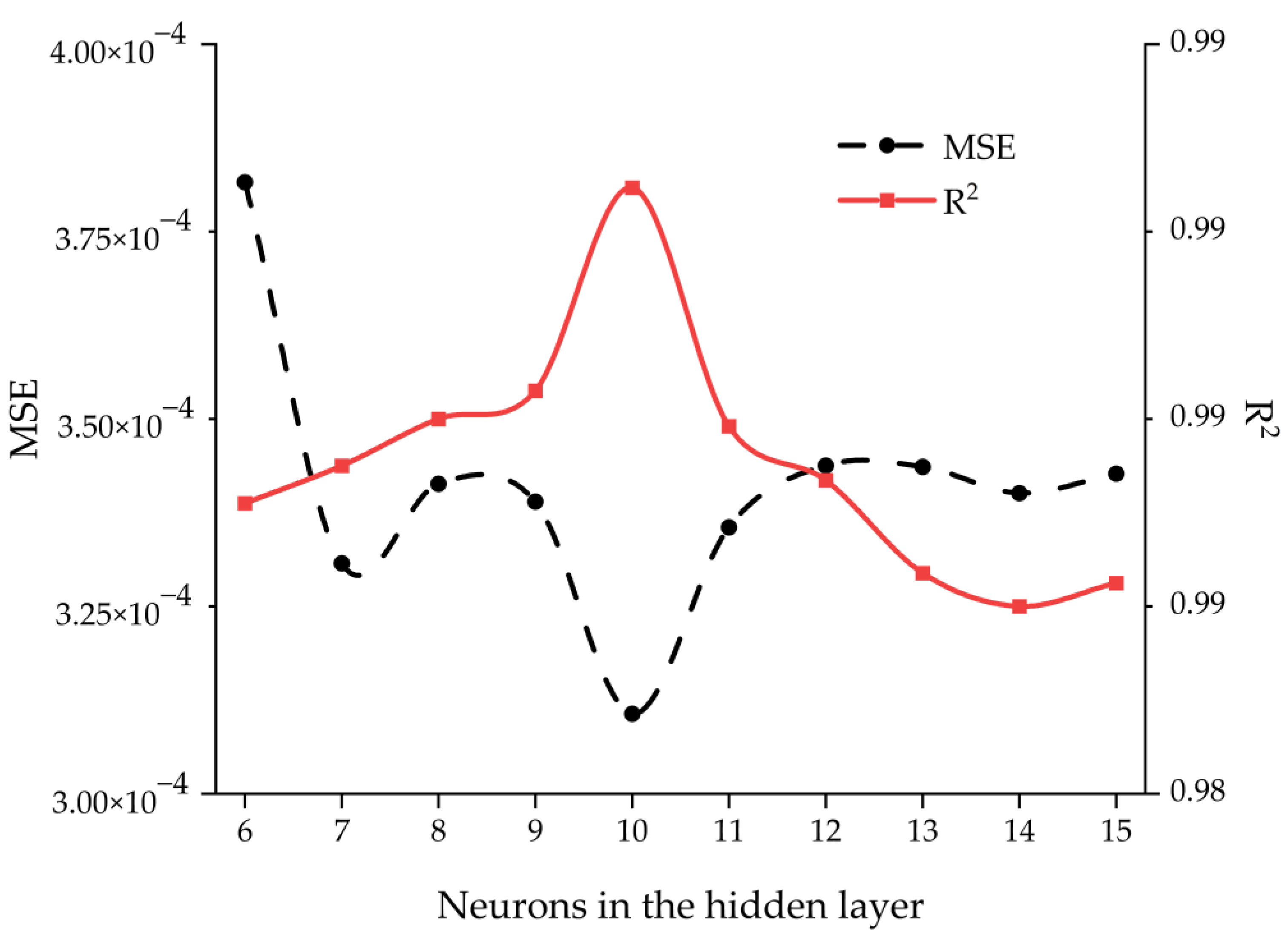
4.3. Hyper-Parametric Tuning

Before the models were developed, the data were standardized between 0 and 1 to overcome the difficulties of processing data with different measurement units and avoid complications related to extreme values. Then, the data were partitioned randomly into three sets: 70% for training, 15% for validation, and 15% for testing. The training and validation sets were then divided equally into ten-sized subgroups and subjected to a 10-fold cross-validation process. The model tuning parameters were determined using their mean performance across ten validation sets by using nine subsets as training and one subset as a validation set repeatedly for a total of ten times. Last, the data-driven models were developed using all the data from the training and validation sets, and the models’ predictive accuracies were determined using the testing set.

As explained in Section 3.3, the input, output, and hidden layers form the layered structure of ANN. To test the ANN model’s sensitivity, different numbers from 6 to 15 neurons were used in the hidden layer. There is no definitive answer to the question of how many neurons the hidden layer of an ANN model should contain. However, some researchers have suggested that more than twice the number of neurons in the hidden layer should be more than the number of input neurons (input variables) [66]. It has also been reported that the number of neurons generated by this statement does not essentially ensure that the network can be generalized [67]. In particular, the neurons in the hidden layer vary depending upon the problem’s nature and the training patterns’ number and quality [68]. If too few neurons are included in the hidden layers, the network may result in underfitting. If, on the other hand, too many neurons are used in the hidden layers, the network can lead to overfitting. The optimal value of the hidden layer neurons was determined after an initial experiment with ten neurons using the stepwise search method (Figure 6). Thus, we decided to use ten neurons to simplify the network.

The three parameters, including the error term penalty parameter (C), kernel coefficient (γ), and radius (ε), are referred to as the SVR model’s hyperparameters. To avoid under- and overfitting, these hyper-parameters need to be chosen correctly. Chang and Lin [69] defined the kernel coefficient as = 1/K, in which K is the total number of inputs. Therefore, the heating and cooling loads in this study were estimated as γ = 1/5. The parameter C is applied to obtain a trade-off between the model’s complexity and the extent to which variations larger than ε are allowed in the optimization formulation. A small value of C gives little weight to the training data and results in a model with an inadequate fit. In contrast, an excessively large value of C minimizes only the empirical risk and leads to an inadequate fit to the training dataset. In this paper, to determine the optimal values for these hyperparameters (C and ε), a two-step grid search approach with 10-fold cross-validation was used to derive the tuning parameters in the SVR model [70]. In this approach, a coarse grid search was performed first and found that the best C and ε were 3 and 0.2, respectively, with an R² of 0.748 (Figure 7a). Then, a finer grid search with tenfold cross-validation was performed in a zone of values optimized from the coarse grid search. This resulted in 2.5 and 0.04 for C and ε, respectively, with an R² of 0.990 (Figure 7b).

Three user-defined parameters, the number of trees (N_T), the number of splits (N_S), and the individual trees’ depth (D), must be specified for optimization to develop the RF models [71]. In this paper, a stepwise search procedure was performed, and the range of 1–200, 2–10, and 1–50 were considered for the N_T, N_S, and D, respectively. It was found that N_T and N_S did not enhance the model’s performance drastically, so default values of 100 and 2 were chosen for these parameters, respectively. In contrast, D enhanced the prediction results greatly, i.e., for values of D equal to 1 and 10, the models have R² values of 0.630 and 0.993, respectively (Figure 8). After a value of D = 10, there was no considerable improvement in the model’s predictive ability, and therefore, D = 10 was used in further experiments.

4.4. Comparison of the Models

The training, validation, and testing results of the ANN, SVR, and RF models to predict heating and cooling loads are shown in

Table 5. Comparison of the prediction errors of the ANN, SVR, and RF models for heating and cooling loads.

	Models	Training			Validation			Testing
		R2	RMSE (kWh)	MAPE (%)	R2	RMSE (kWh)	MAPE (%)	R2	RMSE (kWh)	MAPE(%)
Heating loads	ANN	0.987	0.795	4.147	0.987	0.802	4.148	0.986	0.806	4.152
	SVR	0.988	0.732	3.655	0.988	0.737	3.730	0.988	0.741	3.729
	RF	0.990	0.692	3.245	0.990	0.697	3.334	0.990	0.695	3.328
Cooling loads	ANN	0.995	7.116	3.383	0.994	7.131	3.415	0.994	7.149	3.466
	SVR	0.995	6.923	3.171	0.995	6.956	3.198	0.995	6.979	3.209
	RF	0.997	6.476	2.603	0.996	6.442	2.612	0.996	6.514	2.624

. The table shows clearly that the RF model was more precise than the others during the testing period according to the criteria used: RMSE = 0.695 and 6.514 kWh, MAPE = 3.328 and 2.624%, and R² = 0.990 and 0.996 for heating and cooling loads, respectively.

A Taylor diagram was used as well to examine the R and SD between the predicted and calculated heating and cooling loads for the ANN, SVR, and RF models. This is shown in Figure 9a,b for all models considered, where the RMSE difference is measured as a function of the distance from the reference point (i.e., the calculated value). The point with the highest R and lowest RMSE is the most excellent predictive model. The visual representation of the model reveals that the results of the RF model match the calculated data points much better than those of the ANN and SVR models.

Figure 10 depicts the cumulative frequency of data points as a function of absolute relative deviation for the ANN, SVR, and RF models, which allowed a visual evaluation of these models. A model’s precision and robustness increase with the distance between its curve and the vertical axis. As Figure 10a,b shows, the RF models have greater accuracy, followed by the SVR and ANN models.

Physical models are based on thermodynamic laws that cannot be applied to every existing building due to the large amount of input data and computational effort required to run a detailed energy model [24]. The data-driven approach, on the other hand, learns from historical or available data sets for prediction. The hybrid approach combines physical modeling and the data-driven approach by using the output of physical modeling as the main data sets for building data-driven models. It has the potential to provide a solution to missing building energy consumption data by using physical models to create data sets.

Numerous studies conducted on energy consumption have confirmed that machine learning models have a good predictive ability. Tien Bui et al. [72] used ANN to develop individual models to assess heating and cooling loads in buildings. For this purpose, an appropriate data set was provided, consisting of relative compactness, surface area, wall area, roof area, overall height, orientation, glazing area, and distribution of glazing area. As a result of the study, the models achieved values of R², MAE, and RMSE of 0.902 and 0.918, 2.938 and 3.286 kW, and 3.648 and 3.949 kW for the heating and cooling loads, respectively. Similarly, Moradzadeh et al. [40] used the same inputs to predict the heating and cooling loads of residential buildings. The authors developed SVR models with the following parameters: R (0.998 and 0.988), MAE (0.778 and 1.476 kW), and RMSE (0.885 and 1.739 kW) for heating and cooling loads, respectively. Chou and Bui [37] also used the same inputs in their study and found that SVR + ANN had higher prediction accuracy (RMSE = 1.566 kW, MAE = 0.973 kW, and MAPE = 3.455%) compared to the other individual models they used to predict cooling load. The SVR model predicted the heating load best according to the indices (RMSE = 0.346 kW, MAE = 0.236 kW, and MAPE = 1.132%). Furthermore, several studies have been reported in the literature using machine learning methods with different inputs to predict heating and cooling loads [73,74,75,76].

The best artificial intelligence techniques to estimate energy consumption need to be compared because it is known well that the best data-driven approaches cannot be selected in advance. This study demonstrated that ANN, SVR, and RF are valuable machine-learning methods to predict poultry buildings’ energy consumption. However, the RF model’s performance metrics (RMSE, MAPE, and R²) were superior to those of the ANN and SVR models.

Further, the model developed was integrated into a software module that enables users to make informed energy consumption decisions, detect differences between predicted and expected energy use, determine root causes, and identify and diagnose system errors. In future studies, another promising new approach, Deep Learning, needs to be explored to improve further the accuracy with which energy consumption in poultry buildings can be predicted.

5. Conclusions

Energy forecasting is critical for building managers and owners to make informed decisions. Today, researchers have developed models to predict residential and commercial energy use because energy is so important in our lives. However, no attempt has been made to develop models for poultry houses that consume significant amounts of energy. To fill this gap, energy consumption models were developed in this study using various data-driven techniques (ANN, SVR, and RF). The capabilities of the models studied were tested thoroughly using three statistical parameters, RMSE, MAPE, and R². In addition, graphic evaluations of the performance of the models studied were performed. Based upon the results above, the following conclusions can be drawn:

ANN, SVR, and RF are effective data-driven techniques to predict poultry building energy consumption

Of the models studied, the RF model outperformed the others during the testing period based upon the criteria: RMSE = 0.695 and 6.514 kWh, MAPE = 3.328 and 2.624%, and R² = 0.990 and 0.996 for heating and cooling loads, respectively

Of particular note, the results of this study, which is the first to present data-driven methods to predict poultry buildings’ energy consumption, provide a data-driven pathway to understand building energy consumption and efficiency, and ultimately help building owners and designers achieve better energy savings during planning and renovation. Future efforts should investigate the capability of deep learning models to predict the energy consumption of poultry buildings.

References

1. Küçüktopcu, E.; Cemek, B. The use of artificial neural networks to estimate optimum insulation thickness, energy savings, and carbon dioxide emissions. Environ. Prog. Sustain. 2021, 40, e13478. [Google Scholar] [CrossRef]
2. Roy, S.S.; Roy, R.; Balas, V.E. Estimating heating load in buildings using multivariate adaptive regression splines, extreme learning machine, a hybrid model of MARS and ELM. Renew. Sustain. Energy Rev. 2018, 82, 4256–4268. [Google Scholar]
3. Meng, X.; Yan, B.; Gao, Y.; Wang, J.; Zhang, W.; Long, E. Factors affecting the in situ measurement accuracy of the wall heat transfer coefficient using the heat flow meter method. Energy Build. 2015, 86, 754–765. [Google Scholar] [CrossRef]
4. Huang, H.; Zhou, Y.; Huang, R.; Wu, H.; Sun, Y.; Huang, G.; Xu, T. Optimum insulation thicknesses and energy conservation of building thermal insulation materials in Chinese zone of humid subtropical climate. Sustain. Cities Soc. 2020, 52, 101840. [Google Scholar] [CrossRef]
5. Açıkkalp, E.; Kandemir, S.Y. A method for determining optimum insulation thickness: Combined economic and environmental method. Therm. Sci. Eng. Prog. 2019, 11, 249–253. [Google Scholar] [CrossRef]
6. Küçüktopcu, E.; Cemek, B. A study on environmental impact of insulation thickness of poultry building walls. Energy 2018, 150, 583–590. [Google Scholar] [CrossRef]
7. Verichev, K.; Zamorano, M.; Carpio, M. Effects of climate change on variations in climatic zones and heating energy consumption of residential buildings in the southern Chile. Energy Build. 2020, 215, 109874. [Google Scholar] [CrossRef]
8. Huo, T.; Ren, H.; Cai, W. Estimating urban residential building-related energy consumption and energy intensity in China based on improved building stock turnover model. Sci. Total Environ. 2019, 650, 427–437. [Google Scholar] [CrossRef]
9. Pan, Y.; Zhang, L. Data-driven estimation of building energy consumption with multi-source heterogeneous data. Appl. Energy 2020, 268, 114965. [Google Scholar] [CrossRef]
10. Balaras, C.; Droutsa, K.; Argiriou, A.; Asimakopoulos, D. Potential for energy conservation in apartment buildings. Energy Build. 2000, 31, 143–154. [Google Scholar] [CrossRef]
11. Zhao, H.-x.; Magoulès, F. A review on the prediction of building energy consumption. Renew. Sustain. Energy Rev. 2012, 16, 3586–3592. [Google Scholar] [CrossRef]
12. Paudel, S.; Elmitri, M.; Couturier, S.; Nguyen, P.H.; Kamphuis, R.; Lacarrière, B.; Le Corre, O. A relevant data selection method for energy consumption prediction of low energy building based on support vector machine. Energy Build. 2017, 138, 240–256. [Google Scholar] [CrossRef]
13. Fumo, N.; Mago, P.; Luck, R. Methodology to estimate building energy consumption using EnergyPlus benchmark models. Energy Build. 2010, 42, 2331–2337. [Google Scholar] [CrossRef]
14. Yang, J.; Fu, H.; Qin, M. Evaluation of different thermal models in EnergyPlus for calculating moisture effects on building energy consumption in different climate conditions. Procedia Eng. 2015, 121, 1635–1641. [Google Scholar] [CrossRef] [Green Version]
15. Boyano, A.; Hernandez, P.; Wolf, O. Energy demands and potential savings in European office buildings: Case studies based on EnergyPlus simulations. Energy Build. 2013, 65, 19–28. [Google Scholar] [CrossRef]
16. Ciancio, V.; Falasca, S.; Golasi, I.; Curci, G.; Coppi, M.; Salata, F. Influence of input climatic data on simulations of annual energy needs of a building: EnergyPlus and WRF modeling for a case study in Rome (Italy). Energies 2018, 11, 2835. [Google Scholar] [CrossRef] [Green Version]
17. Kim, D.-B.; Kim, D.D.; Kim, T. Energy performance assessment of HVAC commissioning using long-term monitoring data: A case study of the newly built office building in South Korea. Energy Build. 2019, 204, 109465. [Google Scholar] [CrossRef]
18. Mathews Roy, A.; Prasanna Venkatesan, R.; Shanmugapriya, T. Simulation and analysis of a factory building’s energy consumption using eQuest software. Chem. Eng. Technol. 2021, 44, 928–933. [Google Scholar] [CrossRef]
19. Farzan, H. The study of thermostat impact on energy consumption in a residential building by using TRNSYS. J. Renew. Energy Environ. 2019, 6, 15–20. [Google Scholar]
20. Tsanas, A.; Xifara, A. Accurate quantitative estimation of energy performance of residential buildings using statistical machine learning tools. Energy Build. 2012, 49, 560–567. [Google Scholar] [CrossRef]
21. Tang, W.; Wang, H.; Lee, X.-L.; Yang, H.-T. Machine learning approach to uncovering residential energy consumption patterns based on socioeconomic and smart meter data. Energy 2022, 240, 122500. [Google Scholar] [CrossRef]
22. Amasyali, K.; El-Gohary, N. Machine learning for occupant-behavior-sensitive cooling energy consumption prediction in office buildings. Renew. Sustain. Energy Rev. 2021, 142, 110714. [Google Scholar] [CrossRef]
23. Anand, P.; Deb, C.; Yan, K.; Yang, J.; Cheong, D.; Sekhar, C. Occupancy-based energy consumption modelling using machine learning algorithms for institutional buildings. Energy Build. 2021, 252, 111478. [Google Scholar] [CrossRef]
24. Robinson, C.; Dilkina, B.; Hubbs, J.; Zhang, W.; Guhathakurta, S.; Brown, M.A.; Pendyala, R.M. Machine learning approaches for estimating commercial building energy consumption. Appl. Energy 2017, 208, 889–904. [Google Scholar] [CrossRef]
25. Kharseh, M.; Nordell, B. Sustainable heating and cooling systems for agriculture. Int. J. Energy Res. 2011, 35, 415–422. [Google Scholar] [CrossRef]
26. Amasyali, K.; El-Gohary, N.M. A review of data-driven building energy consumption prediction studies. Renew. Sustain. Energy Rev. 2018, 81, 1192–1205. [Google Scholar] [CrossRef]
27. Moon, J.; Kim, J. ANN-based thermal control methods for residential buildings. Build. Environ. 2010, 45, 1612–1625. [Google Scholar] [CrossRef]
28. Moon, J.W.; Jung, S.K.; Lee, Y.O.; Choi, S. Prediction performance of an artificial neural network model for the amount of cooling energy consumption in hotel rooms. Energies 2015, 8, 8226–8243. [Google Scholar] [CrossRef] [Green Version]
29. Deb, C.; Eang, L.S.; Yang, J.; Santamouris, M. Forecasting diurnal cooling energy load for institutional buildings using Artificial Neural Networks. Energy Build. 2016, 121, 284–297. [Google Scholar] [CrossRef]
30. Melo, A.; Fossati, M.; Versage, R.; Sorgato, M.; Scalco, V.; Lamberts, R. Development and analysis of a metamodel to represent the thermal behavior of naturally ventilated and artificially air-conditioned residential buildings. Energy Build. 2016, 112, 209–221. [Google Scholar] [CrossRef]
31. Ahmad, M.W.; Mourshed, M.; Rezgui, Y. Trees vs Neurons: Comparison between random forest and ANN for high-resolution prediction of building energy consumption. Energy Build. 2017, 147, 77–89. [Google Scholar] [CrossRef]
32. Li, Z.; Dai, J.; Chen, H.; Lin, B. An ANN-based fast building energy consumption prediction method for complex architectural form at the early design stage. Build. Simul. 2019, 12, 665–681. [Google Scholar] [CrossRef]
33. Kalogirou, S.A.; Bojic, M. Artificial neural networks for the prediction of the energy consumption of a passive solar building. Energy 2000, 25, 479–491. [Google Scholar] [CrossRef]
34. Kavaklioglu, K. Modeling and prediction of Turkey’s electricity consumption using support vector regression. Appl. Energy 2011, 88, 368–375. [Google Scholar] [CrossRef]
35. Oğcu, G.; Demirel, O.F.; Zaim, S. Forecasting electricity consumption with neural networks and support vector regression. Procedia Soc. Behav. Sci. 2012, 58, 1576–1585. [Google Scholar] [CrossRef] [Green Version]
36. Jain, R.K.; Smith, K.M.; Culligan, P.J.; Taylor, J.E. Forecasting energy consumption of multi-family residential buildings using support vector regression: Investigating the impact of temporal and spatial monitoring granularity on performance accuracy. Appl. Energy 2014, 123, 168–178. [Google Scholar] [CrossRef]
37. Chou, J.-S.; Bui, D.-K. Modeling heating and cooling loads by artificial intelligence for energy-efficient building design. Energy Build. 2014, 82, 437–446. [Google Scholar] [CrossRef]
38. Zhong, H.; Wang, J.; Jia, H.; Mu, Y.; Lv, S. Vector field-based support vector regression for building energy consumption prediction. Appl. Energy 2019, 242, 403–414. [Google Scholar] [CrossRef]
39. Li, X.; Yao, R. A machine-learning-based approach to predict residential annual space heating and cooling loads considering occupant behaviour. Energy 2020, 212, 118676. [Google Scholar] [CrossRef]
40. Moradzadeh, A.; Mansour-Saatloo, A.; Mohammadi-Ivatloo, B.; Anvari-Moghaddam, A. Performance evaluation of two machine learning techniques in heating and cooling loads forecasting of residential buildings. Appl. Sci. 2020, 10, 3829. [Google Scholar] [CrossRef]
41. Hansen, L.; Salamon, P. Neural network ensembles. IEEE Trans. Pattern Anal. Mach. Intell. 1990, 12, 993–1001. [Google Scholar] [CrossRef] [Green Version]
42. Dietterich, T.G. Ensemble methods in machine learning. In Multiple Classifier Systems; Kittler, J., Roli, F., Eds.; Springer: Berlin/Heidelberg, Germany, 2000; Volume 1857, pp. 1–15. [Google Scholar]
43. Ho, T.K. The random subspace method for constructing decision forests. IEEE Trans. Pattern Anal. Mach. Intell. 1998, 20, 832–844. [Google Scholar]
44. Statnikov, A.; Wang, L.; Aliferis, C.F. A comprehensive comparison of random forests and support vector machines for microarray-based cancer classification. BMC Bioinform. 2008, 9, 1–10. [Google Scholar] [CrossRef] [PubMed]
45. Lahouar, A.; Slama, J.B.H. Day-ahead load forecast using random forest and expert input selection. Energy Convers. Manag. 2015, 103, 1040–1051. [Google Scholar]
46. Yan, L.; Hu, P.; Li, C.; Yao, Y.; Xing, L.; Lei, F.; Zhu, N. The performance prediction of ground source heat pump system based on monitoring data and data mining technology. Energy Build. 2016, 127, 1085–1095. [Google Scholar] [CrossRef]
47. National Chicken Council Animal Welfare Guidelines and Audit Checklist for Broilers. Available online: https://www.nationalchickencouncil.org/policy/animal-welfare/ (accessed on 15 November 2022).
48. CIGR. Heat and moisture production at animal and house level. In 4th Report of Working Group on Climatization of Animal Houses; Pedersen, S., Sallvik, K., Eds.; Danish Institute of Agricultural Sciences: Horsens, Denmark, 2002. [Google Scholar]
49. Ross 308 Performance Objectives. 2019. Available online: http://eu.aviagen.com/tech-center/download/1339/Ross308-308FF-BroilerPO2019-EN.pdf (accessed on 15 November 2022).
50. Wang, Y.; Li, B.; Liang, C.; Zheng, W. Dynamic simulation of thermal load and energy efficiency in poultry buildings in the cold zone of China. Comput. Electron. Agric. 2020, 168, 105127. [Google Scholar] [CrossRef]
51. Hornik, K.; Stinchcombe, M.; White, H. Multilayer feedforward networks are universal approximators. Neural Netw. 1989, 2, 359–366. [Google Scholar]
52. Jalili Ghazi Zade, M.; Noori, R. Prediction of municipal solid waste generation by use of artificial neural network: A case study of Mashhad. Int. J. Environ. Res. 2008, 2, 13–22. [Google Scholar]
53. Atkinson, P.M.; Tatnall, A.R. Introduction neural networks in remote sensing. Int. J. Remote Sens. 1997, 18, 699–709. [Google Scholar] [CrossRef]
54. Haykin, S.S. Neural Networks and Learning Machines, 3rd ed.; Pearson Education: Upper Saddle River, NJ, USA, 2009. [Google Scholar]
55. Yadav, N.; Yadav, A.; Kumar, M. An Introduction to Neural Network Methods for Differential Equations, 1st ed.; Springer: Dordrecht, The Netherlands, 2015. [Google Scholar]
56. Gholami, R.; Fakhari, N. Support Vector Machine: Principles, Parameters, and Applications. In Handbook of Neural Computation; Samui, P., Sekhar, S., Balas, V.E., Eds.; Academic Press: Cambridge, MA, USA, 2017; pp. 515–535. [Google Scholar]
57. Hosseinzadeh, A.; Moeinaddini, A.; Ghasemzadeh, A. Investigating factors affecting severity of large truck-involved crashes: Comparison of the SVM and random parameter logit model. J. Saf. Res. 2021, 77, 151–160. [Google Scholar] [CrossRef]
58. Vapnik, V. The Nature of Statistical Learning Theory; Springer: New York, NY, USA, 1995. [Google Scholar]
59. Vapnik, V.; Golowich, S.E.; Smola, A.J. Support vector method for function approximation, regression estimation and signal processing. In Proceedings of the 9th International Conference on Neural Information Processing Systems, Denver, CO, USA, 3–5 December 1996; Mozer, M.C., Jordan, M., Petsche, T., Eds.; MIT Press: Cambridge, UK, 1996; pp. 281–287. [Google Scholar]
60. Breiman, L. Random forests. Mach. Learn. 2001, 45, 5–32. [Google Scholar] [CrossRef] [Green Version]
61. Hastie, T.; Tibshirani, R.; Friedman, J.H.; Friedman, J.H. The Elements of Statistical Learning: Data Mining, Inference, and Prediction, 2nd ed.; Springer: New York, NY, USA, 2009. [Google Scholar]
62. Cengel, Y.A.; Boles, M.A.; Kanoğlu, M. Thermodynamics: An Engineering Approach, 5th ed.; McGraw Hill: New York, NY, USA, 2006. [Google Scholar]
63. Williams, B.; Onsman, A.; Brown, T. Exploratory factor analysis: A five-step guide for novices. Australas. J. Paramed. 2010, 8, 1–13. [Google Scholar] [CrossRef] [Green Version]
64. Henson, R.K.; Roberts, J.K. Use of exploratory factor analysis in published research: Common errors and some comment on improved practice. Educ. Psychol. Meas. 2006, 66, 393–416. [Google Scholar] [CrossRef] [Green Version]
65. Tabachnick, B.G.; Fidell, L.S. Using Multivariate Statistics, 5th ed.; Allyn & Bacon/Pearson Education: Boston, MA, USA, 2007. [Google Scholar]
66. Hecht-Nielsen, R. Theory of the backpropagation neural network. In Neural Networks for Perception; Wechsler, H., Ed.; Academic Press: Cambridge, MA, USA, 1992; pp. 65–93. [Google Scholar]
67. Rafiq, M.; Bugmann, G.; Easterbrook, D. Neural network design for engineering applications. Comput. Struct. 2001, 79, 1541–1552. [Google Scholar] [CrossRef]
68. Li, Q.; Meng, Q.; Cai, J.; Yoshino, H.; Mochida, A. Predicting hourly cooling load in the building: A comparison of support vector machine and different artificial neural networks. Energy Convers. Manag. 2009, 50, 90–96. [Google Scholar] [CrossRef]
69. Chang, C.-C.; Lin, C.-J. LIBSVM: A library for support vector machines. ACM Trans. Intell. Syst. Technol. 2011, 2, 1–27. [Google Scholar] [CrossRef]
70. Yu, P.-S.; Chen, S.-T.; Chang, I.F. Support vector regression for real-time flood stage forecasting. J. Hydrol. 2006, 328, 704–716. [Google Scholar] [CrossRef]
71. Daviran, M.; Maghsoudi, A.; Ghezelbash, R.; Pradhan, B. A new strategy for spatial predictive mapping of mineral prospectivity: Automated hyperparameter tuning of random forest approach. Comput. Geosci. 2021, 148, 104688. [Google Scholar] [CrossRef]
72. Tien Bui, D.; Moayedi, H.; Anastasios, D.; Kok Foong, L. Predicting heating and cooling loads in energy-efficient buildings using two hybrid intelligent models. Appl. Sci. 2019, 9, 3543. [Google Scholar] [CrossRef] [Green Version]
73. Irshad, K.; Zahir, M.H.; Shaik, M.S.; Ali, A. Buildings’ Heating and Cooling Load Prediction for Hot Arid Climates: A Novel Intelligent Data-Driven Approach. Buildings 2022, 12, 1677. [Google Scholar] [CrossRef]
74. Sholahudin, S.; Han, H. Simplified dynamic neural network model to predict heating load of a building using Taguchi method. Energy 2016, 115, 1672–1678. [Google Scholar] [CrossRef]
75. Kwok, S.S.; Lee, E.W. A study of the importance of occupancy to building cooling load in prediction by intelligent approach. Energy Convers. Manag. 2011, 52, 2555–2564. [Google Scholar] [CrossRef]
76. Jihad, A.S.; Tahiri, M. Forecasting the heating and cooling load of residential buildings by using a learning algorithm “gradient descent”, Morocco. Case Stud. Therm. Eng. 2018, 12, 85–93. [Google Scholar] [CrossRef]
Figure 1. Poultry production cycles.
Buildings 13 00142 g001
Figure 2. Flowchart of the predictive modeling procedure in this study.
Buildings 13 00142 g002
Figure 3. Graphical view of EnergyPlus model.
Buildings 13 00142 g003
Figure 4. The minimum, mean, and maximum values of the EnergyPlus model for different (a) climate zones, (b) wall types, (c) insulation thickness, and (d) insulation thermal conductivity.
Buildings 13 00142 g004aBuildings 13 00142 g004b
Figure 5. Heatmap displaying factor loadings from the exploratory factor.
Buildings 13 00142 g005
Figure 6. Relation between the number of neurons in the hidden layer and mean square error (MSE).
Buildings 13 00142 g006
Figure 7. MSE of SVR optimization for (a) coarse grid search and (b) finer grid search.
Buildings 13 00142 g007
Figure 8. The parameter of depth in RF optimization by stepwise search.
Buildings 13 00142 g008
Figure 9. Taylor diagrams of the predicted (a) heating and (b) cooling loads in testing data.
Buildings 13 00142 g009
Figure 10. Cumulative frequency vs. absolute percent relative error for the models studied for (a) heating and (b) cooling loads in testing data.
Buildings 13 00142 g010