Abstract
For the surface defects inspection task, operators need to check the defect in local detail images by specifying the location, which only the global 3D model reconstruction can’t satisfy. We explore how to address multi-type (original image, semantic image, and depth image) local detail image synthesis and environment data storage by introducing the advanced neural radiance field (Nerf) method. We use a wall-climbing robot to collect surface RGB-D images, generate the 3D global model and its bounding box, and make the bounding box correspond to the Nerf implicit bound. After this, we proposed the Inspection-Nerf model to make Nerf more suitable for our near view and big surface scene. Our model use hash to encode 3D position and two separate branches to render semantic and color images. And combine the two branches’ sigma values as density to render depth images. Experiments show that our model can render high-quality multi-type images at testing viewpoints. The average peak signal-to-noise ratio (PSNR) equals 33.99, and the average depth error in a limited range (2.5 m) equals 0.027 m. Only labeled images of 2568 collected images, our model can generate semantic masks for all images with 0.957 average recall. It can also compensate for the difficulty of manual labeling through multi-frame fusion. Our model size is 388 MB and can synthesize original and depth images of trajectory viewpoints within about 200 m2 dam surface range and extra defect semantic masks.
1. Introduction
Dams are the most critical water conservation project and will result in significant loss of life and property if it fails. China had 98,002 reservoirs in December 2011, with a combined storage capacity of around 930 billion m3. Dam quality and overtopping caused the failure of 3498 dams between 1954 and 2006 [].
Due to long-term scouring, the spillway surface of the Three Gorges Dam has many defects shown in Figure 1. The traditional manual observations approach can identify and estimate the type and size of defects and record location information. During the manual inspection, operators will take some defect images in specific locations for subsequent confirmation and analysis. However, due to the spillway’s low accessibility, it is difficult to achieve sufficient detection and recording of all sidewall surface information manually. Some researchers use more automatic solutions like drones to collect 2D images and multi-view geometry methods to convert 2D images to 3D models. Khaloo’s [] study used the structure from motion (SFM) method to make a general 3D dam model. By resolving better, surface flaws can be found that are as small as a millimeter []. Khaloo uses Hue space color to determine how gravity dams structure changes []. Angeli gives operators an easy way to mark defects by building a dense point cloud on the dam’s surface []. And some researchers only used images and the set calibration facilities to build the overall point cloud model of the dam [,]. Image stitching can also be used for the part of the dam that is downstream, for re-creating images of the dam’s sidewalls, and for the part of the dam that is underwater [,]. In our past work, we used the SLAM method to reconstruct cracks in the sidewalls of drift spillways []. In addition to monitoring through the global model, technicians must repeatedly verify the designated area’s precise local images, not only confirming the position and type of defects.
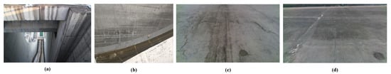
Figure 1.
Dam spillway environment and surface image collection. (a) shows the top view of draft spillway in Three Gorges Dam. (b) shows the image collection status using climbing robot. (c,d) shows typical surface defect collection pictures by climbing robot.
Corresponding global models to detailed local images is a mapping from 3D to 2D, which is the reverse of 3D model reconstruction. To address this reverse procedure, we apply the Nerf method, a state-of-the-art 2D image synthesis method, and propose our Inspection-Nerf approach to adapt to the inspection task. After specifying the local viewpoint position, the corresponding local multi-type images can be rendered, including depth images, semantic label images, and original images. The specific contents of the chapters are as follows. Section 2 introduces works related to concrete surface inspection and Nerf. Section 3 introduces collecting image data and building a global point cloud model using a wall-climbing robot. Section 4 introduces the Inspection-Nerf method. Section 5 presents the experimental tests on the surface of the Three Gorges Dam’s spillways. Section 6 provides a summary and outlook for future research. The contribution of our work can be summarized as follows:
- We propose a double-branches multilayer perceptron (MLP) Nerf structure, which can render multi-type images of all local viewpoints of inspection trajectory. And as we know, we are the first research to introduce radiance fields to big concrete surface scene inspection areas;
- When there are enough training images in a single scene, our model can also be used as a scene storage container, and the main information of 200 m2 of surface data can be retained using only 388 MB of storage space;
- We propose a ranged semantic depth error to measure the depth accuracy of semantic information within a defined distance during multitask rendering.
2. Related Works
2.1. Global Concrete Surface Inspection Related Approaches
The large concrete surface inspection research mainly focuses on the semantic segmentation of defects and environment reconstruction. For semantic segmentation studies of defects, AlexNet is used by Yeum et al. to detect post-disaster collapse, spalling, building column, and facade damage []. Gao diagnoses spalling, column, and shear damage with VGG and Transfer learning []. Li et al. detect cracks and rebar exposure using Faster R-CNN []. Gao section tunnel fractures and leaks utilizing Faster R-CNN and FCN []. Tunnel spalls and cracks are segmented using Inspection-Net []. Hong looks for a better Inspection-Net loss function []. Zhang employs YOLO and FCN for quick crack, spalling, and rebar segmentation []. Several studies have established datasets related to concrete defects. Azimi and Eslamlou et al. outline defect detection and segmentation datasets [], and Yang creates a semantic segmentation datasets of concrete surface spalling and cracks (CSSC) []. Environment reconstruction methods are divided into 2D image stitching and 3D reconstruction methods. Image stitching is an option for re-creating images of the dam’s sidewalls and for the part of the dam that is underwater [,]. But most researchers use 3D approaches. Jahanshahi reconstructs the 3D point cloud of flaws on walls using the method of keyframes paired with SFM to create a surface semantic model of concrete buildings []. Yang performs a 3D semantic reconstruction of the tunnel surface by connecting the CRF fusion method to the semantic segmentation model using the TSDF between keyframes []. This mesh model is helpful for the subsequent defect measuring and assessment. In our earlier work, we built a 3D model of the dam surface using ORB-SLAM2 [] for localization and mapping and neural networks for crack segmentation. Insa-Iglesias develops a remote real-world monitoring system for tunnel inspection using SFM in conjunction with virtual reality []. Hoskere et al. propose a framework using a non-linear finite element model to create a virtual visual inspection testbed using 3D synthetic environments that can enable end-to-end testing of autonomous inspection strategies [].
However, global model-based methods do not achieve a reverse generation from global to local detail images. On the other hand, the inference time of segmentation will increase with the addition of the image sequence length. For multi-class defects, the segmentation accuracy cannot reach the level of manual labeling. And most of the research for defect segmentation needs to construct its own environment dataset. To this end, we propose the Inspection-Nerf method, which only needs to manually label 2% (59/2568) of the typical images in the long sequence. After that, the depth, semantics, and original images of all sequence images can be rendered through training, providing convenience for technicians in the post-inspection, such as defect recheck out and measurement.
2.2. Neural Radiance Field
The Nerf method [] synthesizes 2D images from different viewpoints of a given object by inputting multiple images. Nerf effectively makes 3D viewpoints correspond to 2D images, and many outstanding improvement methods and practical applications have been produced by modifying the encoding method, sampling method, and output type. Yu proposes Plenoctrees [] to improve image rendering speed by converting the implicit radius field to an explicit representation and uses spherical harmonics(SH) to present the RGB values at a location. NeuS [] describes a better 3D geometric representation of the scene by replacing the original density value with the signed distance field (SDF) value and deriving the corresponding sampling equation. Nerf-wild [] constructs multiple MLP networks and variance loss functions to cull transient objects in the scene. NGP [] by hashing the multi-resolution grid in 3D space, the training speed of the scene is greatly improved. Semantic-Nerf [] renders a scene with labels by adding semantic output parallel to density values. Mip-Nerf [] improves the fineness of the rendered image by re-encoding and sampling the frustum, not rays. Mega-nerf [] divides the 2D image collection of a large scene into different regions and then uses multiple small Nerf networks to train each part separately.
To efficiently synthesize multi-type images (original, semantic, and depth images) of the dam surface from different viewpoints, we proposed Inspection-Nerf methods based on the NGP and semantic Nerf. We present a multi-branches(semantic and color heads) structure to render designated viewpoint semantic and color images. After that, we combine two branch density outputs by a linear layer to synthesize corresponding consistent depth images.
3. Data Collection and Preparation
Three steps need to be completed to obtain a local image of a specified viewpoint. First, a stable, precise, close-up image of the spillway sidewall surface is acquired. Then, build a global 3D model of the environment. Finally, ensure the global coordinates can map to the input position-encoded coordinates of the neural radiation field model, as shown in Figure 2.
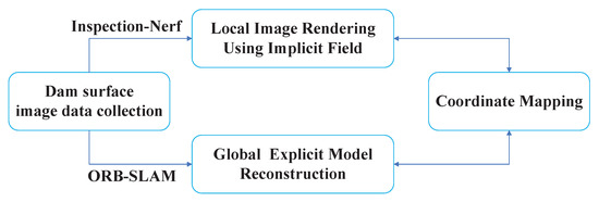
Figure 2.
Flowchart of the proposed global-to-local view synthesis.
3.1. Data Collection by Climbing Robot
There are many ways to obtain information on 3D surfaces, including RGB-D cameras, stereo, time-of-flight, structured light cameras, and LiDAR-based method. We use wall-climbing robots to obtain stable close-up surface information. For outdoor light and moving robot conditions, the use of structured light cameras and time-of-flight cameras is not considered. Stereo requires subsequent point cloud registration, and the algorithm cost required to generate a dense 3D point cloud is greater than that of an RGB-D camera. LiDAR is the first choice for obtaining accurate three-dimensional information in most outdoor conditions. But image information is also needed for Nerf rendering, and it is necessary to equip a monocular, which puts more pressure on the load capacity of the wall-climbing robot. For this reason, using lightweight RGB-D cameras is a better choice for wall-climbing robots to obtain three-dimensional and color information on the wall.
We use a negative-pressure adsorption wall-climbing robot as shown in Figure 1b, carrying an Realsense D435i RGB-D camera, Intel, Santa Clara, CA, USA (the color and depth images’ resolution is 480 × 848 and the frame rate is 30 frames per second), to stably crawl on the surface of the sidewall of the Three Gorges Dam’s drift spillways. The robot is secured by a safety rope and powered by a power cord. We operate the robot move on the dam’s vertical surface and collect sequence images through the robot operation system (ROS). We choose some typical images with multi-class defects and label them as shown in Figure 3.
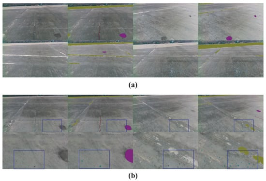
Figure 3.
Image collection and labeling. The collection’s original images are shown in the first and third columns. Labeled images are shown in the second and fourth columns. (a) shows the original images themselves, (b) the second row shows zoom-in visualization of the first row in the blue box. Labeled defects include cracks in red, patched areas in ochre, erosion in purple, and spots in nattier blue.
3.2. Global Model Generation
Following our previous research [], we use the ORB-SLAM method to extract keyframes from the acquired color and depth images and obtain the pose transform matrices of all images. Then, a dense environment point cloud model is generated by bundle adjustment. If the input color image has a class label, the corresponding color of the label can be registered in the point cloud model.
3.3. Global-to-Local Coordinate Mapping
The spatial encoding of Nerf input is continuous, and the boundary can be set manually. Usually, the 3D’s range of the position encoding of the neural radiation field is set to . For the neural network using the normalized device coordinates (NDC), equals 1.0. The global point cloud model is discrete, corresponding to the world coordinate system, and has no boundary restrictions. We need to set the boundary for the global point cloud model and then perform the corresponding transform to convert the points’ coordinates from the global to the implicit local model.
Therefore, after obtaining the global 3D point cloud, the minimum bounding box is obtained by the oriented bounding box (OBB) method []. Then, is transformed into axis-aligned bounding box . Next, obtain the center coordinate of and direction lengths , , along each axises, move the origin to . Finally, calculate the ratio between the longest axis and the set implicit neural field bound value , and scale the bounding box of the 3D point cloud to the implicit model within limits. As shown in Figure 4, the final coordinate transform from the 3D point cloud to the boundary range of the neural radiation field is expressed as the Equation (1). present the rotation transform from global point cloud to OBB coordinate, present the rotation transform from OBB coordinate to AABB coordinate. represents the point coodinate in the real world from the beginning.
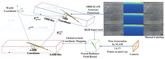
Figure 4.
Global-to-local coordinate mapping. Establish our global-to-local inspection methods. After collecting surface RGB-D images, we label surface defects as shown in the right column using the same color as Figure 3. Using ORB-SLAM to generate images pose and global point cloud and register labeled images to point cloud. After that, use Equation (1) to transform points from the global coordinate to AABB coordinate. Finally, scale the AABB box to the neural radiance field bounding box. (The coordinate origins of OBB box and AABB box are coincident. For the convenience of observation, they are drawn separately in the figure).
4. Methods
4.1. Nerf Principle
The input of Nerf are points position on image pixel rays and corresponding ray direction vector , x denotes the 3D sample point’s position, and is a unit vector representing the sample ray’s direction. The outputs render RGB images from different viewpoints. Then, the Nerf can present a 5D scene as a MLP network as shown in Figure 5. present the volume density and c present the volume RGB color. After supervised training to optimize its weight , Nerf can map each input 5D coordinate to its corresponding density and directional color. The implementation of Nerf comprises three parts: position encoding, sampling strategy, and color rendering equation. The color rendering equation is the core, as shown in Equation (2). The predicted color is obtained by weighting the color of the sampling points along the ray direction. The weight value of the sampling point is represented by the density difference in the sampling interval .
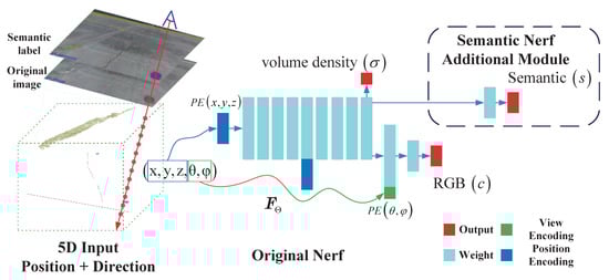
Figure 5.
Nerf structure and data flow. Nerf uses 5D (position and direction) vector as the input. Position and direction using different encoding modules. The outputs are density and RGB values. Semantic Nerf adds a semantic MLP layer after the same feature layers the RGB’s MLP inputs.
The position encoding is divided into two parts. The 3D sample points and ray directions are asymmetrically encoded in high dimensions. The sample points encoding dimension is higher than the direction encoding dimension, which can synthesize higher-quality images []. within the preset range of and . The implicit point sampling in Equation (2) adopts the coarse-fine method. The coarse operation samples implicit points in the ray direction uniformly. Then, the density value of coarse sampling points is used to fit the probability density function(PDF) on the ray direction. Finally, using the coarse-generated PDF to perform fine sampling to get sampling points more accurately.
4.2. Inspection-Nerf Structure
Conventional Nerf and its improved methods are primarily used for image synthesis of small scenes. To achieve fast training of large scenes, we use the multi-resolution position hash encoding method of NGP. Figure 6 shows that different MLP branches are used to output and , respectively. The spatial distance field value uses a learnable linear unit to weigh the two branch distance fields, which can improve the accuracy of depth image rendering. Then, through the NeuS conversion method in Equation (3), the distance field is converted into the density field representation of Nerf. is the Sigmoid function. The final depth prediction equation is expressed as Equation (4). denotes the sample point i’s distance to the camera center.
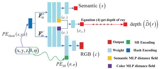
Figure 6.
Inspection-Nerf structure.
The feature output of the semantic MLP branch is used as the input of the classification MLP. Finally, the probability of each category is output through the Softmax layer. After the features of the color MLP branch are concatenated with the features encoded in the SH direction, the predicted values of RGB are obtained through a color rendering MLP layer. The integral equations of semantic labels and color values are shown in Equations (5) and (6). Color and semantic rendering using different MLP networks ( in Equation (5)). denotes the semantic logits of a given volume in Equation (6). The color rendering equation is same as Equation (2).
4.3. Bounding Box Sampling
According to the AABB range and its corresponding transform with the implicit Nerf model, we can directly calculate the sampling ranges and of each pixel ray using the AABB collision detection method []. This approach doesn’t need to input each image’s sampling distance range in advance. The pixel i’s ray can present as . Due to AABB box is axis-aligned, the two points on the diagonal of the cube can represent the six plane coordinates of the cube. Then we calculate the candidate sample distance , j belongs to denote the two diagonal point of AABB cube. is a vector including coordinates. Then, the sample range can be presented as Equation (7).
4.4. Loss Function
In addition to Nerf’s original RGB color loss, we add a depth loss function using the same L1 loss pattern in Equation (8) as color loss does. X in denotes color rendering function or depth rendering function. And semantic loss function in Equation (9) is the conventional cross-entropy loss. Finally, the loss function is formed. , , and are the weight values of the corresponding loss function. R presents the image rays set, and r presents the specific ray belonging to R.
5. Experiments
5.1. Data Preparation
We used a wall-climbing robot equipped with an Intel Realsense D435i RGB-D camera collecting 2568 pairs of images on the side walls of the spillway, including color images and depth images. Then, we select 65 color images with typical defects for defect labeling. Defect types include cracks, erosion, patched area, and spots.
During the global model-building process, the SLAM method generates the pose matrix of each image. We chose 2441 color images as the training set containing 59 semantically labeled images. Other 127 images are used as test images, with 6 semantic labeling images. Part of the defect labeling images and original images are shown in Figure 3. The actual coverage of the dam sidewall by the image collection is 17 × 13 m. Figure 7 shows the camera trajectory positions of training, validation, and labeling images. To see the points of the training image pose clearly, only in (a) do we show one-fifth of the trajectory points.
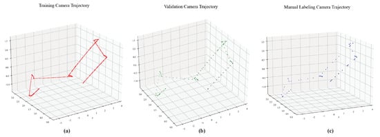
Figure 7.
Camera trajectory during the climbing robot collection process. (a–c) use red, green and blue dots to represent the viewpoint position information of the training, validation, and human-labeled pictures after the robot captures the images.
5.2. Model Implement
Our Inspection-Nerf model has three parts. First, for embedding points and directions, we use the setup of the NGP model. The resolution level is 16, the upper limit of the maximum hash parameter of each level is set to , number of features is 2. And direction embedding, we follow PlenOctree setting and use SH to encode direction color. Second, the semantic and color MLP branches use two layer MLPs with 64 dimensions. Third, rendering part, we use the NeuS sample method, using the mid-points of the N sample points to convert the distance field to neural radiance field. The sampled points use rendering function to calculate each result at last. Using the Adam This is just an optimized general algorithm name. Most papers use their titles directly, and we suggest that no additional information be added. (Adaptive Moment Estimation) optimizer, the learning rate is set to , the weight decay is set to , the learning rate gradually decreases with the number of training iterations, and the Nvidia RTX A6000 GPU (Santa Clara, CA, USA) is used for training 100 epoch. We also set a termination condition during the training process. In addition to the upper limit of 100 epochs, there is also a depth loss that needs to be reduced within less than five epochs, which indicates that the model continues to learn the correct scene depth information. The final model always learns better depth information until 100 epochs are over. Each image selects 8192 pixels per epoch for training. For images with semantic information, the ratios of , , , and are used to randomly select cracks, erosion, patched area, and spots. The proportion of semantic pixels does not exceed of the total number of pixels per epoch, and the background pixel ratio is . When the total number of semantic pixels is insufficient, it is supplemented with background pixels. The weight parameters of the color, semantic, and depth loss functions are set to , , and , requiring 12 minutes per epoch to train. Our model size is 388 MB.
5.3. Metrics and Result
We choose the NGP method combined with semantic Nerf as the baseline with depth loss equals 0.001 (). Original image, semantic image, and depth image rendering results are compared for the dam scene. Figure 8 shows training and validation typical results. In addition to the baseline model, we also compare the Inspection-Nerf training results under three different loss function ratios, including depth loss equals 0.001 (), 0.01 (), and 0.01 depth loss adding sparsity loss [] as regularization (). Figure 8a presents the depth loss changing during the training process, all depth losses are normalized finally. Figure 8b presents the training PSNR. Inspection-Nerf with 0.001 depth loss weight has a higher PSNR value than the baseline, and they have similar depth loss around 0.008. Furthermore, all Inspection-Nerf-based models have faster convergence rates than the baseline models, reaching higher PSNR values about 40 epochs earlier. Nerf-related methods are only trained to render a single scene, so we use the model parameters of the last epoch as the best model to validate later.
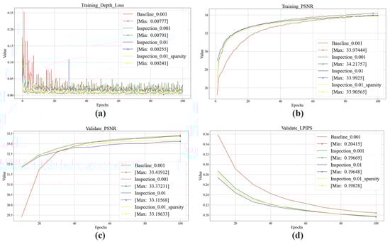
Figure 8.
Training and validation results. (a,b) depict changes in depth loss and average PSNR during training, respectively. (c,d) depict the averaged PSNR and LPIPS metrics during validation testing.
We use the PSNR and LPIPS parameters as the original image rendering evaluation indicators. Figure 8c,d shows the validation PSNR and LPIPS values. Baseline and Inspection-Nerf-based models with the same depth loss weight have the best and second best validation PSNR, and Inspection-Nerf models have better LPIPS validation values. Similar to the training process, Inspection-Nerf models also have faster convergence rates than baseline models in the validation process. We test the number of level equals to 11 versus the original 16. According to the NGP method, the number level equals 11 means the resolution is , which is enough to meet the implicit representation of the actual length of 17 m (real resolution around 0.0167 m) on the longest side of the experimental environment. And we also test the original Nerf model, which uses traditional position embedding (cosine and sine embedding in 10 digits). The results are shown in the last two rows in Table 1. The original Nerf uses trigonometric functions to encode large scenes, and the sparsity of spatial encoding makes the model unable to represent the details of large scenes well. Under hash coding, when the number level is equal to 11, it can also achieve high-precision RSDE indicators while ensuring a certain color rendering quality. For a complete visualization, we compare the rendering results of all models in Appendix A.

Table 1.
Color and depth rendering metrics comparison of different models and loss settings. second best ↑ or ↓ best ↑↑ or ↓↓.
For the depth image, we examine the depth error of the defect category area within a specific distance range, which we call ranged semantic depth error (RSDE) in Equation (10). is the intersection of pixels within distance threshold and defect pixels. I denotes the pixel in images. The smaller the error, the more accurately technicians can measure the defect within the threshold at post-procedure. The RSDE of different methods are shown in the third column of Table 1, we set the equals to 2.5 m. The green cell means the second-best metric, and the yellow cell means the best metric. Inspection-Nerf using 0.01 as a weight for depth loss has the best LPIPS and RSDE metrics.
For the evaluation of semantic image results, the artificial labeling as ground truth sometimes cannot identify the semantic information of distant locations while rendered images can. So we intuitively compare rendered images of different methods with artificial labeling images, as shown in Figure 9. Each group of pictures is arranged in rows in the order of manual labeling, baseline, and . The first column presents original images, the second column presents depth images, and the last column shows semantic images. The column side of the original column is the zoom-in detail of original images.
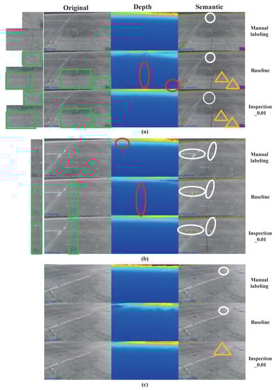
Figure 9.
Multi-type rendering results comparison with manual labeling of validation data. (a–c) depict the rendered image results from different viewpoints. The green box marks the comparison of the original image rendering. The red ellipse marks the comparison of the depth rendering. The white circle marks that the Nerf models can recover further semantic information than manual labeling. The orange triangle marks the comparison of the semantic rendering results of different models.
The green boxes in the original columns show that the Inspection-Nerf model can render spots and crack on the surface in more detail than baseline models. The red ellipses in the depth column indicate that the baseline model usually renders depth values inaccurately within the semantic area, especially crack areas. Our model’s depth results within semantic areas are as accurate as the ground truth. On the semantic column of Figure 9, white ellipses indicate semantic information that is missing or ignored when manually labeling. Due to viewing angle limitations, manual labeling often overlooks defects at long distances. Cracks are ignored in (a)–(b), and erosion labels are ignored in (c). After training on images collected in sequence, Nerf-based methods can recover the long-distance neglected semantic information in a single image through multi-view input. The orange triangles in (a) and (c) show that Inspection-Nerf can retrieve more semantic information than the baseline. It indicates that Inspection-Nerf has learned more scene semantic structure information, which is more conducive to grasping complete surrounding environment semantic information when viewing local details. In order not to lose generality, we also count the average recall and f1-score of Inspection-Nerf for manual labeling defects, which are 0.958 and 0.778, respectively. This shows that our model can not only retain most of the semantic information of human labels but also make up for the information ignored by human labels.
For unlabeled images, Nerf-based methods can also recover semantic information. As shown in Figure 10, these images have no manual labeling for training. We can compare it with Figure 9a,b and Figure 10a,b. Since it is sparsely labeled, Figure 10a,b around the manual labeled Figure 9a,b has no semantic information. Through training, our model can restore the semantics of the images in the surrounding unlabeled viewpoint area, and the semantic recovery information is better than the baseline model. The upper orange ellipse in Figure 10a is intended to represent the recovery of distant semantic information, and our method is also better than the baseline. The reason for this phenomenon is that, as seen from the predicted depth map, the proposed method versus baseline provides more smoothes the depth prediction of distant information, which may make it easier for the model to map semantic information to specific locations, making semantic prediction more complete. The orange circles show that Inspection-Nerf can retrieve more semantic information than the baseline model. Finally, Inspection-Nerf can generate all 2568 collection images’ semantic masks only using 59 labeled images as semantic ground truth to train. Our model can synthesize 1.6 GB original and depth images from different trajectory viewpoints only using 388 MB parameters. And semantic mask images for all images can be generated additionally.
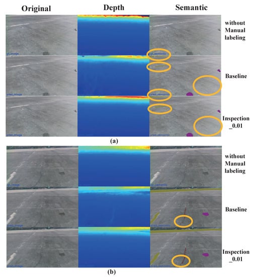
Figure 10.
Multi-type rendering results comparison without manual labeling of validation data. The orange ellipse in (a) marks the restoration comparison of the long-distance patched area and short-distance spot semantics, and the semantic restoration comparison of crack defects is marked in (b).
5.4. Sparse Images Sequence Training Experiment
In theory, the 388 MB parameter of the Inspection-Nerf model is to encode the 3D space in the AABB. Therefore, within the scope of AABB, the more trajectory images are input, the more accurate the rendering result will be. At the same time, it is also stated that the 388 MB model can be used to generate more rendered images within the same AABB range. We validate by sparse the number of training trajectory images. The training sequence images are set to 2311 (90%), 2054 (80%), and 1284 (50%) images, respectively, and the results are shown in Table 2. To increase the credibility of semantic segmentation, we added 50 new human-labeled semantic images to the original 6 semantic test images.
Table 2.
Sparse sequence input training results.
The original training procedure uses 2441 images () to train. The column represents all sequence images, including training and validation. represents the validation image sequence, , and mode use the same validation sets as the original mode does. 50% of the data in the training mode produce noticeable quality degradation. For semantic part, we compare and results to check the recall and accuracy of the model against human labels. The column represents all human labeling images, which is total 115, and denotes the validation image set, which is total 56. We can see that the more semantic labeling images contained in the training set, the more accurately model can recall and predict the defect label in the validation set.As seen in Table 2 the bold first line shows the original setting has the best results in all indicators. So, if we have more image data within the fixed AABB 3D range, we can render multi-type images with the same level of accuracy using the 388 MB model.
6. Conclusions and Future Work
We introduce the state-of-the-art image synthesis method Nerf to address the problem of scene storage and image rechecking from global to local in the dam surface inspection task. Our model’s hash position encoding and double-branches structure can render more detailed and accurate color, depth, and semantic images. And only needing labeled images, the model can synthesize semantic masks with high defect recall for all input scene images. All these contributions only take 388 MB of storage. Mainly, using the same size model, the more input images used to train, the more realistic result can be synthesized. It effectively assists the data store and technicians in surface inspection task process and improves the human-computer interaction performance of the inspection process. Our future work will focus on unifying the explicit global and implicit local models to improve inspection automation ability.
Author Contributions
Conceptualization, K.H.; methodology, K.H.; software, K.H.; validation, K.H.; formal analysis, K.H.; investigation, K.H. and H.W.; resources, K.H. and B.Y.; data curation, K.H.; writing—original draft preparation, K.H.; writing—review and editing, K.H.; visualization, K.H.; supervision, H.W.; project administration, H.W.; funding acquisition, H.W. All authors have read and agreed to the published version of the manuscript.
Funding
The authors would like to acknowledge the financial support by the China Yangtze Power Co., Ltd. and Shenyang Institute of Automation, Chinese Academy of Sciences (Contract/Purchase Order No.E249111401). This research was also supported in part by Shenyang Institute of Automation, Chinese Academy of Sciences, 2022 Basic Research Program Key Project(Highly Adaptable Robot Design Method for Complex Environment and Multi-task).
Institutional Review Board Statement
Not applicable.
Informed Consent Statement
Not applicable.
Data Availability Statement
Data available on request due to restrictions privacy.
Acknowledgments
We appreciate the site and equipment support provided by China Yangtze Power Co., Ltd. in the process of the wall climbing robot test.
Conflicts of Interest
The authors declare no conflict of interest.
Abbreviations
The following abbreviations are used in this manuscript:
| MDPI | Multidisciplinary Digital Publishing Institute |
| DOAJ | Directory of open access journals |
| TLA | Three letter acronym |
| LD | Linear dichroism |
| Nerf | Neural radiance field |
| PSNR | Peak signal-to-noise ratio |
| LPIPS | Learned perceptual image patch similarity |
| SFM | Structure from motion |
| SLAM | Simultaneous location and mapping |
| MLP | Multilayer perceptron |
| CSSC | Concrete surface spalling and cracks |
| SDF | Signed distance field |
| RSDE | Ranged semantic depth error |
Appendix A. Supplementary Comparison of Multi-Model Rendering Results
To better demonstrate the comparison of the rendering results between the various models, here we show a multi-model image rendering result.

Figure A1.
All model rendering result comparison of a validation image.
References
- Shi-Qiang, H. Development and prospect of defect detection technology for concrete dams. Dam Saf. 2016, 4, 1. [Google Scholar]
- Khaloo, A.; Lattanzi, D.; Jachimowicz, A.; Devaney, C. Utilizing UAV and 3D computer vision for visual inspection of a large gravity dam. Front. Built Environ. 2018, 4, 31. [Google Scholar] [CrossRef]
- Ghahremani, K.; Khaloo, A.; Mohamadi, S.; Lattanzi, D. Damage detection and finite-element model updating of structural components through point cloud analysis. J. Aerosp. Eng. 2018, 31, 04018068. [Google Scholar] [CrossRef]
- Khaloo, A.; Lattanzi, D. Automatic detection of structural deficiencies using 4D Hue-assisted analysis of color point clouds. In Dynamics of Civil Structures; Springer: Berlin/Heidelberg, Germany, 2019; Volume 2, pp. 197–205. [Google Scholar]
- Angeli, S.; Lingua, A.M.; Maschio, P.; Piantelli, L.; Dugone, D.; Giorgis, M. Dense 3D model generation of a dam surface using UAV for visual inspection. In Proceedings of the International Conference on Robotics in Alpe-Adria Danube Region, Patras, Greece, 6–8 June 2018; pp. 151–162. [Google Scholar]
- Buffi, G.; Manciola, P.; Grassi, S.; Barberini, M.; Gambi, A. Survey of the Ridracoli Dam: UAV–based photogrammetry and traditional topographic techniques in the inspection of vertical structures. Geomat. Nat. Hazards Risk 2017, 8, 1562–1579. [Google Scholar] [CrossRef]
- Ridolfi, E.; Buffi, G.; Venturi, S.; Manciola, P. Accuracy analysis of a dam model from drone surveys. Sensors 2017, 17, 1777. [Google Scholar] [CrossRef] [PubMed]
- Oliveira, A.; Oliveira, J.F.; Pereira, J.M.; De Araújo, B.R.; Boavida, J. 3D modelling of laser scanned and photogrammetric data for digital documentation: The Mosteiro da Batalha case study. J. Real-Time Image Process. 2014, 9, 673–688. [Google Scholar] [CrossRef]
- Sakagami, N.; Yumoto, Y.; Takebayashi, T.; Kawamura, S. Development of dam inspection robot with negative pressure effect plate. J. Field Robot. 2019, 36, 1422–1435. [Google Scholar] [CrossRef]
- Hong, K.; Wang, H.; Zhu, B. Small Defect Instance Reconstruction Based on 2D Connectivity-3D Probabilistic Voting. In Proceedings of the 2021 IEEE International Conference on Robotics and Biomimetics (ROBIO), Sanya, China, 27–31 December 2021; pp. 1448–1453. [Google Scholar]
- Yeum, C.M.; Dyke, S.J.; Ramirez, J. Visual data classification in post-event building reconnaissance. Eng. Struct. 2018, 155, 16–24. [Google Scholar] [CrossRef]
- Gao, Y.; Mosalam, K.M. Deep transfer learning for image-based structural damage recognition. Comput.-Aided Civ. Infrastruct. Eng. 2018, 33, 748–768. [Google Scholar] [CrossRef]
- Li, R.; Yuan, Y.; Zhang, W.; Yuan, Y. Unified vision-based methodology for simultaneous concrete defect detection and geolocalization. Comput.-Aided Civ. Infrastruct. Eng. 2018, 33, 527–544. [Google Scholar] [CrossRef]
- Gao, Y.; Kong, B.; Mosalam, K.M. Deep leaf-bootstrapping generative adversarial network for structural image data augmentation. Comput.-Aided Civ. Infrastruct. Eng. 2019, 34, 755–773. [Google Scholar] [CrossRef]
- Yang, L.; Li, B.; Li, W.; Liu, Z.; Yang, G.; Xiao, J. Deep concrete inspection using unmanned aerial vehicle towards cssc database. In Proceedings of the IEEE/RSJ International Conference on Intelligent Robots and Systems, Vancouver, BC, Canada, 24–28 September 2017; pp. 24–28. [Google Scholar]
- Zhang, C.; Chang, C.c.; Jamshidi, M. Simultaneous pixel-level concrete defect detection and grouping using a fully convolutional model. Struct. Health Monit. 2021, 20, 2199–2215. [Google Scholar] [CrossRef]
- Azimi, M.; Eslamlou, A.D.; Pekcan, G. Data-driven structural health monitoring and damage detection through deep learning: State-of-the-art review. Sensors 2020, 20, 2778. [Google Scholar] [CrossRef] [PubMed]
- Jahanshahi, M.R.; Masri, S.F. Adaptive vision-based crack detection using 3D scene reconstruction for condition assessment of structures. Autom. Constr. 2012, 22, 567–576. [Google Scholar] [CrossRef]
- Yang, L.; Li, B.; Yang, G.; Chang, Y.; Liu, Z.; Jiang, B.; Xiaol, J. Deep neural network based visual inspection with 3d metric measurement of concrete defects using wall-climbing robot. In Proceedings of the 2019 IEEE/RSJ International Conference on Intelligent Robots and Systems (IROS), Macau, China, 3–8 November 2019; pp. 2849–2854. [Google Scholar]
- Mur-Artal, R.; Tardós, J.D. Orb-slam2: An open-source slam system for monocular, stereo, and rgb-d cameras. IEEE Trans. Robot. 2017, 33, 1255–1262. [Google Scholar] [CrossRef]
- Insa-Iglesias, M.; Jenkins, M.D.; Morison, G. 3D visual inspection system framework for structural condition monitoring and analysis. Autom. Constr. 2021, 128, 103755. [Google Scholar] [CrossRef]
- Hoskere, V.; Narazaki, Y.; Spencer Jr, B.F. Physics-Based Graphics Models in 3D Synthetic Environments as Autonomous Vision-Based Inspection Testbeds. Sensors 2022, 22, 532. [Google Scholar] [CrossRef]
- Mildenhall, B.; Srinivasan, P.P.; Tancik, M.; Barron, J.T.; Ramamoorthi, R.; Ng, R. Nerf: Representing scenes as neural radiance fields for view synthesis. Commun. ACM 2021, 65, 99–106. [Google Scholar] [CrossRef]
- Yu, A.; Li, R.; Tancik, M.; Li, H.; Ng, R.; Kanazawa, A. Plenoctrees for real-time rendering of neural radiance fields. In Proceedings of the IEEE/CVF International Conference on Computer Vision, Montreal, BC, Canada, 11–17 October 2021; pp. 5752–5761. [Google Scholar]
- Wang, P.; Liu, L.; Liu, Y.; Theobalt, C.; Komura, T.; Wang, W. Neus: Learning neural implicit surfaces by volume rendering for multi-view reconstruction. arXiv 2021, arXiv:2106.10689. [Google Scholar] [CrossRef]
- Martin-Brualla, R.; Radwan, N.; Sajjadi, M.S.; Barron, J.T.; Dosovitskiy, A.; Duckworth, D. Nerf in the wild: Neural radiance fields for unconstrained photo collections. In Proceedings of the IEEE/CVF Conference on Computer Vision and Pattern Recognition, Nashville, TN, USA, 20–25 June 2021; pp. 7210–7219. [Google Scholar]
- Müller, T.; Evans, A.; Schied, C.; Keller, A. Instant neural graphics primitives with a multiresolution hash encoding. arXiv 2022, arXiv:2201.05989. [Google Scholar] [CrossRef]
- Zhi, S.; Laidlow, T.; Leutenegger, S.; Davison, A.J. In-place scene labelling and understanding with implicit scene representation. In Proceedings of the IEEE/CVF International Conference on Computer Vision, Montreal, BC, Canada, 11–17 October 2021; pp. 15838–15847. [Google Scholar]
- Barron, J.T.; Mildenhall, B.; Tancik, M.; Hedman, P.; Martin-Brualla, R.; Srinivasan, P.P. Mip-nerf: A multiscale representation for anti-aliasing neural radiance fields. In Proceedings of the IEEE/CVF International Conference on Computer Vision, Montreal, BC, Canada, 11–17 October 2021; pp. 5855–5864. [Google Scholar]
- Turki, H.; Ramanan, D.; Satyanarayanan, M. Mega-NeRF: Scalable Construction of Large-Scale NeRFs for Virtual Fly-Throughs. In Proceedings of the IEEE/CVF Conference on Computer Vision and Pattern Recognition, New Orleans, LA, USA, 19–24 June 2022; pp. 12922–12931. [Google Scholar]
- Gottschalk, S.A. Collision Queries Using Oriented Bounding Boxes; The University of North Carolina at Chapel Hill: Chapel Hill, NC, USA, 2000. [Google Scholar]
- Zhang, K.; Riegler, G.; Snavely, N.; Koltun, V. Nerf++: Analyzing and improving neural radiance fields. arXiv 2020, arXiv:2010.07492. [Google Scholar] [CrossRef]
- Cai, P.; Indhumathi, C.; Cai, Y.; Zheng, J.; Gong, Y.; Lim, T.S.; Wong, P. Collision detection using axis aligned bounding boxes. In Simulations, Serious Games and Their Applications; Springer: Berlin/Heidelberg, Germany, 2014; pp. 1–14. [Google Scholar]
Disclaimer/Publisher’s Note: The statements, opinions and data contained in all publications are solely those of the individual author(s) and contributor(s) and not of MDPI and/or the editor(s). MDPI and/or the editor(s) disclaim responsibility for any injury to people or property resulting from any ideas, methods, instructions or products referred to in the content. |
© 2023 by the authors. Licensee MDPI, Basel, Switzerland. This article is an open access article distributed under the terms and conditions of the Creative Commons Attribution (CC BY) license (https://creativecommons.org/licenses/by/4.0/).