Abstract
Large-span open prefabricated spatial grid structures are characterized by light mass, high flexibility, low self-oscillation frequency, and low damping, resulting in wind-sensitive structures. Meanwhile, their height tends to be relatively low, located in the wind field with a large wind speed gradient and high turbulence area. Therefore, surface airflow is complex, and many flow separations, reattachment, eddy shedding, and other phenomena occur, causing damage to local areas. This paper took the Evergrande Stadium in Guiyang, China, as the research object and used the random number cyclic pre-simulation method to study its surface extreme wind pressure. Firstly, five conventional distributions (Gaussian, Weibull, three-parameter gamma, generalized extreme value, and lognormal distribution) were fitted to the wind pressure probability densities at different measurement points on the surface of the open stadium. It is found that the same distribution could not be chosen to describe the probability density distribution of wind pressure at all measurement points. Hence, based on the simulation results, the Gaussian and non-Gaussian regions of this structure were divided to determine where to apply which distribution. Additionally, the accuracy of the peak factor, improved peak factor, and modified Hermite moment model method were compared to check their applicability. Finally, the effect of roughness on the extreme wind pressure distribution on the open stadium surface was also investigated according to the highest accuracy method above. The findings of this study will provide a reference for engineers in designing large-span open stadiums for wind resistance to minimize the occurrence of wind damage.
1. Introduction
Most of the shapes of large-span open prefabricated spatial grid structures are graceful and variable in appearance as three-dimensional blunt bodies. When the airflow reaches the edge of the windward side of the roof, separation and eddy shedding will occur here, and a significant wind absorption area will be formed at the separation and reattachment points. Subsequently, the airflow continues to move along the roof surface, whose movement cannot be coordinated with the unique shape of the roof itself due to the roughness, leading to flow separation and the formation of various eddies. Furthermore, the topography of the building site differs, and the surrounding buildings interfere with the flow field, so the wind field flow characteristics of large-span open prefabricated spatial grid structures are relatively complex. Additionally, such structures are low in height and located in a region of high wind speed variability and turbulence in the atmospheric boundary layer. Large-span roofs are frequently damaged by wind (Figure 1). Currently, the Chinese load code [1] only gives a part of the simple and representative building form factor and fails to consider the wind pressure distribution of complex large-span open prefabricated spatial grid structures in practical engineering [2]. Thus, there is a lack of a reliable basis in the structural design process. It is urgently necessary to find an efficient, stable, and accurate method to obtain the flow characteristics of the wind field on the surface of the structure, the turbulence characteristics of the structure itself, and the pulsation characteristics of the wind load on the surface of the structure.
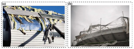
Figure 1.
Example of wind damage to large-span roof structures: (a) Beijing Capital Airport T3 cover was lifted; (b) Zhejiang Jiaxing Pinghu gymnasium cover was torn.
Computational fluid dynamics (CFD), traditional theoretical analysis, and experimental measurement methods are the primary ways to study fluid flow problems [3,4,5,6,7,8]. They form a complete system, both verifying and complementing each other. Nowadays, according to the different methods of solving the Navier–Stokes (N–S) equation and the treatment of various-scale eddies in turbulence, the numerical simulation methods are classified into three categories: direct numerical simulation (DNS), Reynolds averaging (RANS), and large-eddy simulation (LES). The DNS method directly solves the N–S equation, theoretically acquiring all bands of the energy spectrum and the most miniature eddy. However, it requires a sufficiently fine grid and superb computational power and is mainly applied to calculating low Reynolds numbers, and not to the high Reynolds number operation of building flow around. The LES method simulates large- and small-scale eddies, allowing the accurate solution of large-scale turbulent motions and obtaining unsteady structures inaccessible to RANS. However, the critical issue in modeling the flow field around the building with this method is determining the pulsating wind speed inlet conditions. The existing conventional simulation methods are divided into active and pre-simulation methods [9]. The former generates the pulsating wind velocity by artificially satisfying certain conditions into the computational domain entry to simulate the atmospheric boundary layer, while the continuity conditions are hardly satisfied. The principal idea of the latter is to create the wind field using the pre-pre-simulation area and extract the data of the corresponding surface in it. Then, the data from the extraction surface are loaded into the entrance of the master simulation area for calculation, resulting in a relatively realistic flow field structure and spatio-temporal correlation for this approach [10]. Simultaneously, the inlet turbulence characteristics get well maintained in the computational domain because it meets the basic equations of fluid motion. Specifically, Spalar [11] proposed a cyclic pre-simulation method to shorten the length of the computational domain, i.e., the following data extraction surface is cyclically flowed with the inlet by introducing periodic boundary conditions in the downstream direction. By this method, Lund et al. [12] improved the inlet conditions of the pre-simulated wind speed to meet the requirements of shear stress and boundary layer height and enhanced the quality of the generated turbulent flow field. Subsequently, Ferrante et al. [13] utilized the addition of turbulent kinetic energy at the inlet to make the simulated results easier to match requirements. Raupach [14] increased the turbulence degree of the turbulent flow field by adding rough elements in the area of pre-simulation and parametrically analyzed the number and arrangement of rough elements to provide a reference basis for such a method. Wang [15] applied methods such as rough elements and random numbers at the entrance to enhance the turbulence of the flow field and finally obtained a wind field similar to the four types of landforms in the Chinese Code for Structural Loads of Buildings [1].
Regarding the traditional theoretical analysis methods and experimental measurement methods, Davenport [16] proposed the peak factor method in the 1960s based on the assumption that the wind pressure distribution on the building surface conforms to a Gaussian distribution. However, Paterka [17] pointed out that the wind pressure at some parts of the roof (e.g., in the high negative pressure area caused by a conical eddy) showed non-Gaussian characteristics, where the actual wind pressure distribution characteristics failed to be fitted well with the Gaussian distribution. Thus, Kareen and Zhao [18] tried to build a non-Gaussian model closer to the actual pulsating wind pressure. They introduced the non-Gaussian correction term into the non-Gaussian process expressed as a Hermite series polynomial of the Gaussian process and proposed a peak factor calculation method considering higher-order statistics. Subsequently, Kumar K.S and Stathopoulos et al. [19] compared the surface wind pressures of a variety of typical low-roof buildings and found that the absolute values of the skewness coefficients of the wind pressure distribution in certain areas were large. Therefore, an attempt was made to partition the roof wind pressure using Gaussian and non-Gaussian distribution as criteria. Furthermore, Sadek and Simiu [20] applied the transformation process method [21] to map the probability distribution function of the non-Gaussian wind pressure time course into a standard Gaussian distribution based on the zero-value crossing theory [22]. Besides the above extreme-value estimation methods, there is also a way to estimate the wind pressure value based on the wind tunnel test. Kasperski [23] and Homels et al. [24] conducted wind tunnel tests on low-rise buildings to acquire numerous wind pressure time samples and studied their probability distributions, showing that they could be better described by the Gumbel distribution and the extreme-value type I distribution. Although this is the ideal method for extreme-value studies, it requires a considerable sample size of experimental data, leading to expensive costs. Thus, its practical application has many limitations. Basically, the theoretical analysis method can allow for various influencing factors, but it tends to be harder to solve for realistic complex flows and fails to give analytical solutions. The experimental measurement method gives realistic and reliable results, but the wind tunnel test usually suffers from the influence of model size, flow field disturbance and measurement accuracy, and consumes considerable manpower, material and financial resources.
With the above practical situation, this study adopted the random number cyclic pre-simulation method to generate the entrance boundary conditions and applied them to the large-eddy simulation of the TUU standard model. Meanwhile, the comparison of the modeling results with the wind tunnel test and the actual field measurement results was carried out to verify its accuracy and applicability. Next, the surface extreme wind pressure distribution characteristics of typical large-span open prefabricated spatial grid structure (Evergrande Stadium) were investigated. Firstly, wind pressure probability densities at different measurement points on the surface of Evergrande Stadium were fitted using five conventional distributions, and the fitting effects were analyzed. Secondly, the accuracy of the peak factor, improved peak factor, and modified Hermite moment model method for calculating the wind pressure on the surface of this structure was investigated. Finally, the elements influencing the extreme wind pressure distribution on the surface of this stadium, including wind angle and roof roughness, were considered. The findings were expected to serve as a relevant basis for designing wind resistance of large-span open prefabricated spatial grid structures, thereby enabling effective defense against wind damage.
2. Numerical Simulation Methods
2.1. Large-Eddy Simulation (LES)
LES is a method to achieve flow field reproduction using spatial averaging, where filtering occurs on a grid scale to remove high-frequency components of physical quantity calculations. The filtering function is given below:
where indicates spatial coordinates; and represent the volume and coordinate range of the control body, respectively. The following equation can express the large-scale average component :
where stands for flow field area. By processing the continuity and the transient N–S equation through Equation (2), the set of control equations for LES is derived as follows:
where the variables containing the superscript are the spatially averaged components after filtering; is sublattice scale stress, which refers to the influence of small-scale eddies on the motion of large-scale eddies. The following equation can express it:
where means a newly added unknown quantity. Because for the closure of Equation (3), it is necessary to construct the expressions of sublattice scale stresses using the corresponding model.
2.2. Cyclic Pre-Simulation Method
In the atmospheric boundary layer, increasing the number of rough elements and the length of the computational domain downstream is often required to add turbulence to the flow field. However, this will significantly enhance the computational effort of LES. Meanwhile, as the calculation proceeds, the flow velocity of the fluid at the same height will gradually decrease along the downstream direction due to the viscosity of the fluid and the frictional resistance of the wall, making the flow field appear to decay. Therefore, the pseudo-periodic boundary method and random number method were adopted in this paper to shorten the length of the computational domain downstream and enhance the turbulence in the upper part of the flow field. Specifically, the physical quantities on the circulation surface downstream of the computational domain were extracted and assigned to the inlet to achieve fluid flow circulation. The pseudo-periodic boundary condition specified the expression (Equation (5)) for the mean wind speed profile at the entrance and superimposed the pulsation velocity on this profile, as shown in Figure 2.
where , denotes height above ground; equals to atmospheric boundary layer thickness.
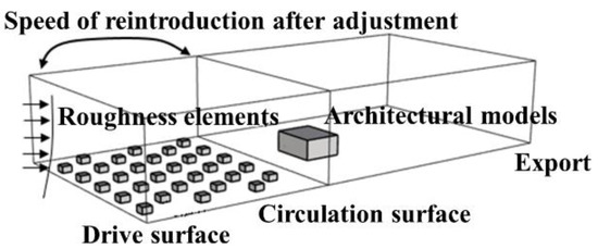
Figure 2.
Schematic diagram of the cyclic pre-simulation method.
This method assumes that the atmospheric boundary layer thickness is constant throughout the computational domain. The purpose of using the weight function is to limit the fluctuation of the pulsating wind high in the calculation domain and stabilize the calculation. Figure 3 plots the variation of the power function with height and atmospheric boundary layer thickness, where the thickness is taken from the thickness of the four types of landforms specified in the GB 50009-2012 [1], respectively, 300 m, 350 m, 450 m, and 550 m. Kataoka simulated a high-rise building with large eddies employing this pseudo-periodic boundary condition, but the turbulence degree was low. Therefore, rough elements were arranged in the atmospheric boundary layer wind field to get higher turbulence of the flow field in this paper.
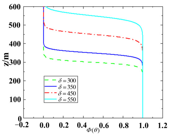
Figure 3.
Variation of the weight function with height above ground and atmospheric boundary layer thickness.
Raupach et al. [25] found that the friction velocity is linked to the density of the rough element, where the rough element density represents the average windward area of the rough element per unit area:
where indicates the number of rough elements in the unit area; and are the width and height of the windward side of the rough element, respectively; represents the total surface area of all rough elements in the unit area. When , Lettau [26,27] presented the existence of a linear relationship between , and :
where 0.5 stands for the average resistance coefficient of a single obstacle. Furthermore, the empirical equation [28] given by ESDU to describe the variation of turbulence is:
where is height-dependent parameters. Both methods are applied to estimate the size and arrangement of the rough elements in the pre-simulation method using the pseudo-periodic boundary conditions. The location of the circulation surface should meet the requirements of the full development of turbulence and minimize the instability caused by the circulation, so generally the distance between the circulation surface and the entrance is taken to be higher than the thickness of the atmospheric boundary layer.
The turbulence derived from LES using the above cyclic pre-simulation method is only elevated near the ground, while the turbulence at a high location will be slight. In wind tunnel tests, increasing the turbulence at high places is usually achieved by adding sharp splits. However, if this approach is adopted in the numerical simulation, it will enormously increase the number of meshes and degrade their quality. Besides, the size and arrangement of the tip split need to be adjusted, resulting in a significant additional calculation. Therefore, this paper adopted the method of adding random numbers at high places to realize its turbulence degree increase, decreasing the computation. Meanwhile, the debugging process is easy and straightforward, and the final turbulence meets the requirements of GB 50009-2012 [1]. Specifically, the root means square of the added random number should be approximately equal to that of the pulsating wind speed. If random numbers satisfy a normal distribution with a mean zero, their standard deviation is as follows:
where denotes the standard deviation of random numbers; refers to target turbulence; is the means turbulence with rough element arrangement only; indicates the average speed in downwind direction. The boundary condition of this random number is superimposed and corrected with the pseudo-periodic boundary condition to obtain the velocity boundary condition at the entrance, as in Equation (10):
2.3. UDF Interface for Loading Inflow Information
For LES, it is difficult to input Fluent software directly for simulation because of the complicated boundary conditions. Therefore, a user-defined function (UDF) interface with Fluent software is required to meet the target turbulence characteristics at the inlet. UDF is applied in this paper to achieve the following functions: (1) generation of random numbers with zero mean normal distribution; (2) extraction of the pulsation velocity of each grid cell on the circulation surface; (3) superimposition of the above pulsation velocity on the mean wind profile of the corresponding grid cell at the entrance; (4) initialization of the flow field; (5) adoption of single-computer multi-core parallel computing to improve the computational efficiency.
2.4. Validation of Numerical Simulation Methods
The TTU building model is a standard model for low-rise buildings in the field of structural wind engineering, as proposed by WERFL, Texas Tech University. Its shape is approximately rectangular and has a smooth surface without any appendages, with the dimension of . Moreover, the top surface has a slope with a slope of 1/60. Currently, the TTU building model has become a more authoritative standard for verifying the simulation technology of building wind tunnels. Plenty of researchers usually perform wind tunnel tests with small-size TTU standard models. The test results are compared with the original data provided by the TTU research team to study the wind field simulation in the atmospheric boundary layer (including inflow characteristics and wind environment), pressure measurement techniques, model size, and wind pressure distribution. Therefore, the TTU standard model is also employed to verify the accuracy of the LES in this paper. Specifically, the way of generating atmospheric boundary layer turbulence by the random number cyclic pre-simulation method described in Section 2.2 was applied to the numerical simulation of the large eddies of the TTU standard model to study the wind pressure distribution at its surface. Also, the simulation results were compared with the field measurements and wind tunnel test values of Texas Tech University to verify the accuracy and applicability of this method in LES.
2.4.1. Simulation of TTU Standard Model
The TTU standard model was put into the wind field with a blockage rate of 3.1%, and the computational domain and coordinate system are shown in Figure 4a,b. Since the TTU standard model is approximately rectangular, the grid adopted a structured grid with good quality (Figure 4c). Grids near the TTU were encrypted, while larger grids were utilized near the exit and the top surface of the computational domain to minimize the computation time. Generally, to ensure that the simulation can capture the delicate eddies at the structure, the thickness of the boundary layer mesh must be small enough to satisfy the dimensionless wall distance . While a tiny time step is required to guarantee that the (Courant–Friedrichs–Lewy), resulting in a waste of computational resources. Because most current simulations utilize implicit computation to discretize the time term, the and requirement can be appropriately relaxed and increased, respectively [29,30,31,32]. The final grid size of the first layer near the wall was 0.0002 m, .
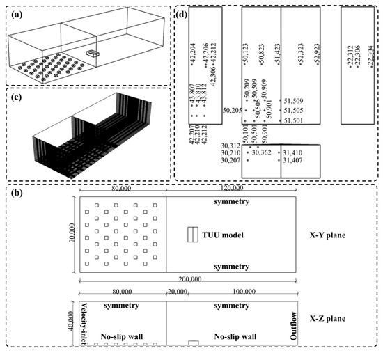
Figure 4.
Calculation domain and measurement point arrangement for numerical simulation: (a) overall view; (b) XY and XZ plane; (c) watershed grid distribution; (d) arrangement of measurement points at the standard height of the TTU model.
2.4.2. Setting of Solution Method and Boundary Conditions
The subgrid model adopted the wall-adaptive local eddy viscosity model in LES with the reference pressure point location set at the top of the TTU standard model. The Pressure-Implicit with Splitting of Operators (PISO) algorithm was selected for the pressure-velocity coupling scheme in the numerical calculation. Because PISO is an extension of the semi-implicit method for pressure-linked equations (SIMPLE), with an additional corrector step, and developed for the non-iterative computation of unsteady compressible flows. Therefore, PISO is more suitable for the unsteady simulation than the SIMPLE algorithm [33]. The spatial and temporal discretization utilized a bounded central difference and second-order fully implicit format, respectively. Considering the CFL conditions, the time step and step number were 0.0002s and 50,000 steps, respectively, obtaining 10s of wind pressure time series data [34]. The boundary conditions were set as shown in Table 1.

Table 1.
Setting of boundary conditions.
2.4.3. Post-Processing Process
The arrangement of the measurement points of the TTU standard model surface is shown in Figure 4d, and their wind pressure time series were extracted in the calculation. For direct analysis, the wind pressure values at the measurement points were transformed into wind pressure coefficients (dimensionless) in this paper, and the average and pulsating wind pressure coefficients at the standard height of the TTU standard model were compared separately. The average wind pressure coefficients are positive and negative values representing wind pressure and suction, respectively. Its calculation formula is as follows:
where and represent the wind pressure coefficient and static pressure value of the measurement point at the time step , respectively; stands for reference wind pressure, usually can be taken as an atmospheric pressure value; is the air density, given as 1.225 kg/m3; denotes average wind pressure coefficient at the measurement point ; means the number of wind pressure time steps extracted from the measurement point. The formula for the pulsating wind pressure coefficient is as in Equation (12):
2.4.4. Analysis of Calculation Results
Wind Fields
Figure 5 compares the mean wind speed profile and flow turbulence profile obtained from LES in this section with the wind tunnel experiments (WT-TJ) results at Tongji University [35] and the field measurements at TTU [36]. It can be seen that they have favorable consistency.
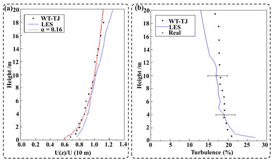
Figure 5.
Comparison of wind fields: (a) mean wind speed profile; (b) flow turbulence profile.
Flow Field
The wind speed vector diagram of the TTU model is illustrated in Figure 6, indicating that wind speed grows with height. Strong flow separation occurs at the eave tip and the airflow reattachment at the middle and rear of the roof, with no airflow separation at the ridge. Meanwhile, three distinct eddies could be observed appearing near the building. Specifically, the first two eddies are located near the windward side near the ground and in the wake area of the leeward wall, and they generate significant pressure and suction effects on the enclosure, respectively. The last eddy created by flow separation above the roof is closest to the building and produces a more significant wind suction force on the roof.
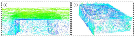
Figure 6.
Average wind speed vector diagram of flow field: (a) overall flow field; (b) TTU model.
Wind Pressure Coefficient
Figure 7 depicts the comparison of the line average, pulsation, and peak wind pressure coefficients in the TTU model in this section (LES) with the experimental data from the TJ-2 wind tunnel at Tongji University (WT-TJ) [35], the field-measured data from TTU (Real) [36] and the wind tunnel experimental data from the University of Western Ontario, Canada (WT-UWO) [37], respectively. Clearly, the average and peak wind pressure coefficients obtained in this section of LES differ slightly from the wind tunnel experimental results, and the pulsation pressure coefficient is marginally smaller on the windward side. Compared with the measured data in the site, the average wind pressure coefficient in LES is in excellent agreement, and the pulsation wind pressure coefficient is slightly more significant on the windward side, while the peak wind pressure coefficient is the opposite. This is because the wind tunnel test uses a scaled-down model, while the LES in this paper adopts a full-scale model, and there is also an inevitable error between the wind tunnel test and the field measurement itself. Therefore, overall, the LES employed in this paper can accurately reflect the dynamic wind pressure on the surface of the building footprint.
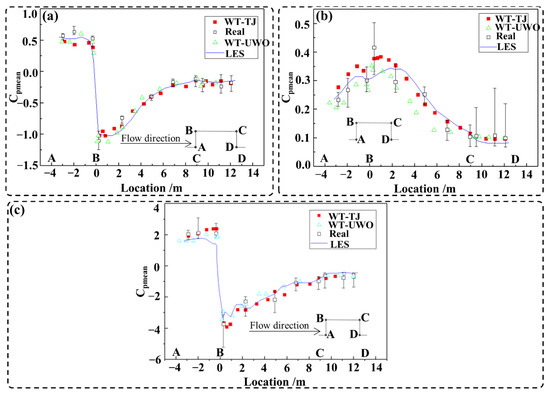
Figure 7.
Comparison of pressure coefficients: (a) average pressure coefficient; (b) pulsation wind pressure coefficient; (c) peak wind pressure coefficient. A-B, B-C, and C-D are the windward wall, roof, and backwind wall, respectively.
3. Characteristics of Extreme Wind Pressure Distribution of the Large-Span Open Prefabricated Spatial Grid Structure
3.1. Introduction of LES for Evergrande Stadium
The stadium is situated in Guiyang City, Guizhou Province, with a short span of 270 m and a long span of 316 m (Figure 8a). Its planar projection is elliptical and strictly symmetric about the X and Y axes. The grandstand part is a circular canopy structure with plenty of steel outer frames protruding from the outer surface of the envelope as a structural support system. The model is subjected to a basic wind pressure of 0.35 kN/m2 and a ground roughness of class B.
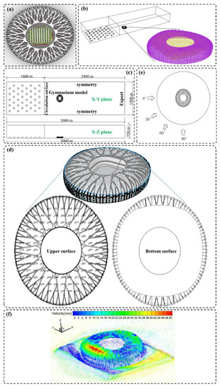
Figure 8.
Stadium rendering and numerical simulation diagram: (a) render graph; (b) computational domain and model surface mesh distribution; (c) XY and XZ plane; (d) model measurement points arrangement; (e) wind direction angle setting; (f) wind speed vector diagram.
The model was foot-ruled, and the computational domain and coordinate system are shown in Figure 8b,c, with a blockage rate of 3.5%. Due to the complex shape of the large-span open prefabricated spatial grid structure, it is not easy to divide the grid. While the rough element has a more regular shape, the computational domain was split into two parts and divided by a mixed mesh. A tetrahedral grid with high-form adaptability was adopted in the region near the stadium. The model surface was set up with six layers of prismatic mesh. The first layer of mesh size near the wall surface was set to 0.001 m, whose value of was less than 70. The grid extension rate was 1.05 to achieve the transition from a dense to a sparse grid in the area near the stadium. Other areas applied structured grids, and the “interface” between the two grids was adopted for data transfer (Figure 8b). In performing LES, the calculation scheme remained identical to Section 2.4.2. The time step and the number of steps were 0.001 s and 20,000, respectively, obtaining 20 s of wind pressure time series data. A total of 504 measurement points were designed on the model surface, where P001 to P312 for the elevation measurement points, P313 to P408 for the upper surface measurement points of the roof, and P409 to P504 for the corresponding bottom surface measurement points of the roof (Figure 8d). The wind direction angle was set as in Figure 8e.
3.2. Distribution Characteristics of Wind Pressure Probability Density
3.2.1. Introduction of Standard Fitting Functions
Gaussian, Weibull, 3P-gamma, GEV, and lognormal distribution are commonly available fitting functions in wind engineering. The primary contents of this section include a brief introduction of the above five distributions and the fitting of wind pressure time-dependent probability density to represent measurement points on the surface of the open prefabricated spatial grid structure.
- (1)
- Gaussian distribution
The Gaussian distribution probability density function is shown below:
where indicates scale parameters; represents position parameters. They can all be solved by using the maximum likelihood estimation method.
- (2)
- Weibull distribution
The Weibull distribution has various distribution forms, such as one-, two- and three-parameter distributions, where the last of these is determined by a combination of shape, scale, and position parameters [38]. The shape parameter decides the shape of the density curve, and the scale parameter plays a scaling role in the shape of the curve and does not impact the shape of the distribution. Its expression is as follows:
where and stand for shape and scale parameters, respectively.
- (3)
- 3P-gamma distribution
- (4)
- GEV distribution
- (5)
- Lognormal distribution
3.2.2. Fitting Results of the Probability Distribution of Representative Measurement Points
In this section, based on the above five probability density functions, the data from the representative measurement points (P330, P360, P426, and P456) on the surface of the model are fitted and analyzed by using the Matlab program for the standard normalization of the wind pressure coefficient time series (Figure 9) [39,40,41,42].
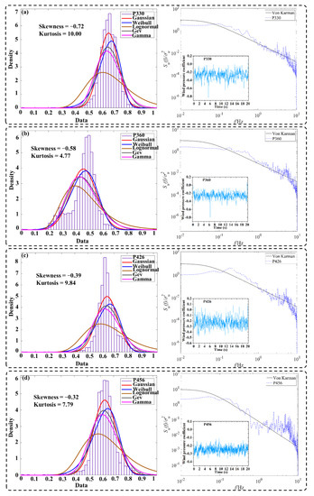
Figure 9.
Probability distribution, wind pressure time series and normalized wind pressure coefficient power spectrum of representative measurement points at 0° wind angle: (a) P330; (b) P360; (c) P426; (d) P456. P330; and P360 refer to the upper surface measurement points of the roof, while P426 and P456 are the bottoms.
For the upper surface measurement points P330 and P360 of the roof, the change in wind angle causes the characteristic turbulence to vary, resulting in a significant difference in the probability distribution for four wind angles. The probability density distributions of the former at different wind angles are steeper at the top and have more apparent asymmetry, consistent with the kurtosis values of this measurement point, which are always higher than 10. The Gaussian distribution cannot fit the wind pressure probability distribution of this measurement point well, while the GEV and 3P-gamma distributions have more excellent results. The kurtosis values of the latter at both 0° and 90° wind angles fall between 4 and 5. Moreover, the probability density distribution is flat at the top of both. The Gaussian and Weibull distributions reasonably fit the wind pressure probability at this measurement point. For the measurement points P426 and P456 on the lower surface of the roof, the probability density distributions at 0° are similar to P330 and P360, and also agree with the larger absolute values of skewness and kurtosis. Furthermore, the wind pressure probability distributions of these two points deviate from the Gaussian distribution relatively seriously, while GEV and 3P-gamma distributions perform effectively. Exceptionally, the probability density distribution of the P456 at a 90° wind angle has an apparent symmetry, in line with the comparatively small value of the measurement point skewness. Moreover, the probability distribution of wind pressure at this measurement point matches well with the Gaussian distribution.
In general, the 3P-gamma and GEV distribution are better to fit because the wind pressure probability density distribution at most measurement points on the surface of the open prefabricated spatial grid structure fails to meet the Gaussianity assumption. For the measurement points with higher absolute values of skewness and kurtosis, both Gaussian and lognormal distributions have non-negligible deviations and poorer fitting effects. Therefore, dividing the surface into Gaussian and non-Gaussian regions is necessary to determine the distribution for different measurement points.
3.2.3. Gaussian and Non-Gaussian Region Division
Sun [43] proposed two criteria to characterize the skewness and kurtosis-taking criteria for non-Gaussian characteristics: (1) the values of skewness and kurtosis should not bias from the skewness and kurtosis center matching curve; (2) the degrees of probability assurance within its variation are close. As shown in Figure 10a, the kurtosis and skewness of all points at different wind angles counted according to the above two guidelines can be fitted with a quadratic function () that satisfies criterion (1). The same criteria can be suggested to classify Gaussian and non-Gaussian regions for open prefabricated spatial grid structure surfaces at different wind angles. On the other hand, the probability densities of satisfying skewness and kurtosis are approximately equal (Figure 10b,c), both around 70%, following criterion (2).
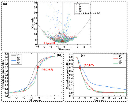
Figure 10.
Results of curve fitting: (a) kurtosis and skewness; (b) beyond probability density of skewness; (c) beyond probability density of kurtosis.
Consequently, the measurement points satisfying skewness and kurtosis were divided into non-Gaussian regions in this section, and the rest belonged to Gaussian regions. According to this criterion, the classification findings are shown in Figure 11. Significantly, at a 30° wind angle, the Gaussian region on the upper surface of the roof is the largest, covering less than half of the total area. In contrast, the maximum Gaussian area is on the lower surface of the roof at a 60° wind angle. Elsewhere, the area occupied by the Gaussian region on the top and bottom surfaces of the roof is minor.
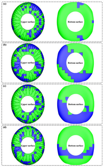
Figure 11.
Division of Gaussian and non-Gaussian regions of the roof under different wind angles: (a) 0°; (b) 30°; (c) 60°; (d) 90°. The blue and green areas are Gaussian and non-Gaussian areas, respectively.
3.3. Comparative Analysis of Extreme Wind Pressure Calculation Methods
This section provides a comparative analysis of the estimation errors of the peak factor, improved peak factor, and modified Hermite moment model method on the extreme wind pressure of open prefabricated spatial grid structures for selecting a reasonable method to serve as a basis for the following study. For a better examination of the estimation accuracy of the three methods, the absolute error rate (Equation (18)) and the average error rate (Equation (19)) were employed.
where represents the total number of measurement points on the surface of the open prefabricated spatial grid structure. The standard extreme wind pressure factor is the average of the observed extreme values (large or small) of the sample. Here, LES was performed six times under the same conditions for 504 measurement points on the surface, and six data samples with all times of 20 s were obtained. The mean of the observed extreme values of the first five samples was treated as the standard value to assess the merits of the extreme values derived from the above three methods for the sixth sample data. From the absolute error rate of each measurement point, it can be seen that with the change in wind angle, a large part of the error rate of the peak factor method and the improved peak factor method for the standard maximum value of wind pressure coefficient is above 20%, and even reaches 80% (Figure 12). Whereas the modified Hermite moment model method gives a more accurate estimation, the error with the coefficient is controlled within the 0–20% range, apparently better than the first two methods. Furthermore, the average error rate of the peak factor method and the improved peak factor method achieves 20–35%, with poor estimation accuracy. The modified Hermite method keeps it well within 10–13% (Figure 13).
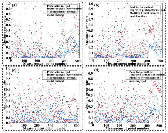
Figure 12.
Absolute error rate of each measurement point: (a) 0° wind direction angle; (b) 30° wind direction angle; (c) 60° wind direction angle; (d) 90° wind direction angle.
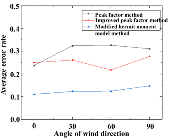
Figure 13.
Average error rate of three methods for estimating the maximum value of wind pressure coefficient.
3.4. Effect of Surface Roughness on the Extreme Wind Pressure Distribution
When the airflow arrives at the edge of the windward side of the open prefabricated spatial grid structure, separation and eddy shedding will occur, and a significant wind suction area will be formed at the separation and reattachment points. Subsequently, the airflow continues to move along the roof surface. Due to the roughness of the roof, its movement cannot be coordinated with the unique shape of the structure itself, leading to flow separation and the formation of various eddies. Therefore, to study the effect of stadium surface roughness on its surface extreme wind pressure distribution, the rough and completely smooth surfaces were set as working cases 1 (roughness height is 1.3 m) and 2, respectively, to explore the differences (Figure 14).
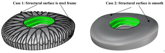
Figure 14.
Diagram of working cases.
3.4.1. Extreme Wind Pressure Distribution
In this section, the extreme wind pressure on the surface of this open prefabricated spatial grid structure was calculated by the modified Hermite moment model method. Figure 15, Figure 16, Figure 17 and Figure 18 show the distribution of the extreme values of wind pressure coefficients at each wind direction angle under working cases one and two, respectively.
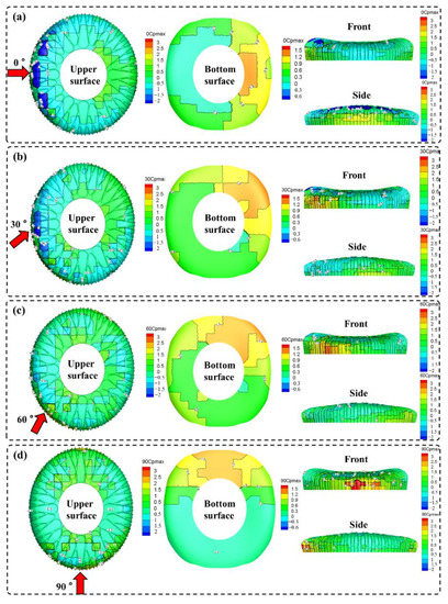
Figure 15.
Maximum value of wind pressure coefficient at each wind direction angle for working case 1: (a) 0°; (b) 30°; (c) 60°; (d) 90°.
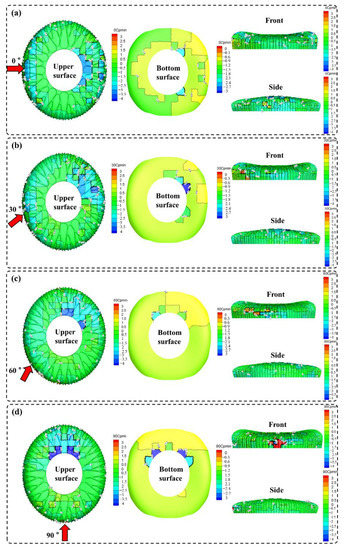
Figure 16.
Minimum value of wind pressure coefficient at each wind direction angles for working case 1: (a) 0°; (b) 30°; (c) 60°; (d) 90°.
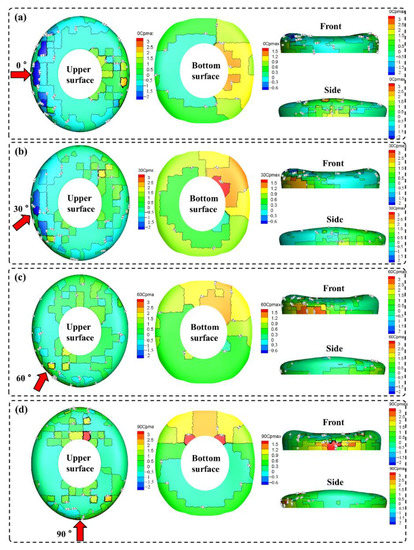
Figure 17.
Maximum value of wind pressure coefficient at each wind direction angle for working case 2: (a) 0°; (b) 30°; (c) 60°; (d) 90°.
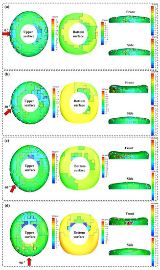
Figure 18.
Minimum value of wind pressure coefficient at each wind direction angle for working case 1: (a) 0°; (b) 30°; (c) 60°; (d) 90°.
Comparing the maximum values of wind pressure coefficients at 0°, 30°, 60°, and 90° wind angles for working case one, it can be seen that: (1) the wind pressure coefficients in the upper surface area of the roof are all less than zero, indicating that it is subject to wind suction. At 0° and 30° wind angles near the edge of the windward area, its values are about −2, and −0.5 at 60° and 90°. This is because the open prefabricated spatial grid structure is saddle-shaped; at 0° and 30° wind angles, the airflow in front of the roof is constantly rising, near the highest point of the roof height it falls suddenly, and the airflow along the edge of the roof shows a strong separation. The roof height in the windward area does not drop suddenly under 60° and 90° wind angles, so the airflow separation phenomenon is insignificant. As a result, the wind suction effect on the region varies with the wind angle, with the wind pressure coefficient being smaller at 0° and 30° and more significant at 60° and 90°. (2) The wind pressure coefficient on the lower surface of the roof is approximately equal in the area for positive and negative regions, and the distribution correlates with the wind direction angle. The part near the windward area is negative, and the surface is subject to wind suction, while the part far away from this area is subject to wind pressure. This indicates that the surface near the windward area generates negative pressure along the airflow direction due to airflow separation. After crossing the opening, the surface away from the windward area experiences positive pressure due to the impulse of airflow, with the local wind pressure coefficient reaching 1.2. (3) The wind pressure coefficient in the windward area of the front and side elevations remains positive. Meanwhile, with the change of wind angle, the position of the maximum wind pressure coefficient changes, the windward area coefficient is always positive, and the maximum value is around 0.5 to 3. It means that as the wind angle changes, the airflow, and the windward side collide and separate, and as a result, the windward elevation area coefficient is always positive and subject to wind pressure. The two sides of the windward elevation are subject to wind suction due to airflow separation.
Comparing the minimum values of wind pressure coefficients at 0°, 30°, 60°, and 90° wind angles for working case one, it can be seen that: (1) the wind pressure coefficients in the upper surface area of the roof are also all less than zero. At 0° and 30° wind angles near the edge of the windward area, its values are about −3, and −4 at 60° and 90°. This is because the open prefabricated spatial grid structure is saddle-shaped; at 0° and 30° wind angle, the airflow in front of the roof constantly rises, near the highest point of the roof height it falls suddenly, and the airflow along the edge of the roof shows a separation. After crossing the openings, it reaches the edge away from the windward area and produces a significant wind suction effect on the surface. The roof height in the windward area does not drop suddenly under 60° and 90° wind angles, so the wind pressure coefficient is more prominent at 0° and 30°, and smaller at 60° and 90°. (2) The wind pressure coefficients of the lower surface area of the roof are less than 0, and the distribution of the area is related to the wind angle. The coefficient of the part near the windward area is smaller, and far from the windward area is more prominent. It means that along the airflow direction, the negative pressure is generated near the windward area due to the airflow separation, and after crossing the openings, the wind suction effect continues far from the windward area. (3) The wind pressure coefficient in the windward area of the front and side elevations remains positive. Meanwhile, with the change in wind angle, the position of the minimum wind pressure coefficient changes, and the maximum value remains positive, at around 1 to 3. It also means that as the wind angle changes, the airflow and the windward side collide and separate, and as a result, in the windward elevation area the coefficient is always positive and subject to wind pressure. The two sides of the windward elevation are subject to wind suction.
Comparing the maximum values of wind pressure coefficients at 0°, 30°, 60°, and 90° wind angles for working case two, similar results were obtained as follows: (1) the wind pressure coefficients in the upper surface area of the roof are all less than zero, indicating that it is subject to wind suction. At 0° and 30° wind angles near the edge of the windward area, its values are about −2, and −0.5 at 60° and 90°. (2) The wind pressure coefficient on the lower surface of the roof is approximately equal in the area for positive and negative regions, and the distribution correlates with the wind direction angle. The part near the windward area is negative, and the surface is subject to wind suction, while the part far away from this area is subject to wind pressure. This phenomenon is the same as in case one, but the local wind pressure coefficient reaches 1.5. (3) The wind pressure coefficient in the windward area of the front and side elevations remains positive. Meanwhile, with the change of wind angle, the position of the maximum wind pressure coefficient changes; the windward area coefficient is always positive, and the maximum value is around 2 to 3.
Comparing the minimum values of wind pressure coefficients at 0°, 30°, 60° and 90° wind angles for working case two, similar results were obtained as follows: (1) the wind pressure coefficients in the upper surface area of the roof are also all less than zero. At 0° and 30° wind angles near the edge of the windward area, its values are about −3, and −4 at 60° and 90°. (2) The wind pressure coefficients of the lower surface area of the roof are less than 0, and the distribution of the area is related to the wind angle. The coefficient of the part near the windward area is smaller, and far from the windward area is more prominent. (3) The wind pressure coefficient in the windward area of the front and side elevations remains positive. Meanwhile, with the change in wind angle, the position of the minimum wind pressure coefficient changes, and the maximum value keeps positive, with around 1.5 to 3.
3.4.2. Analysis of the Effect of Roughness on Extreme Wind Pressure Distribution
In this section, to study the effect of the smooth surface of the gymnasium and the wind angle on the extreme wind pressure on the surface of the open prefabricated spatial grid structure, measurement points (P326–334, P342, P349, P355, P361, P367, P375, P384, P395–387, P379, P372, P366, P360, P354, P346, P337) on the upper surface of the roof were selected for study based on the working cases one and two, respectively (Figure 8 and Table 2 and Table 3). They were sorted by 1–32, and the maximum and minimum values of wind pressure coefficients for the two working cases at each wind angle were extracted in Figure 19 and Figure 20. Clearly, the maximum values of the wind pressure coefficients of working cases one and two at each wind direction angle are approximately equal, and the laws of change with the location of the measurement points are similar. It means that the surface roughness of the open prefabricated spatial grid structure has no noticeable effect on the overall distribution of the extreme value. The maximum values of wind pressure coefficients at points P391 at 0°, P395 at 30°, and P367 at 90° are significantly larger than those at case one, and each measurement point is on the side of the roof away from the windward area. It suggests that the maximum wind pressure of case two in the local area will be stronger than that in case one and should be considered in the structural design. The minimal values of wind pressure coefficients in cases one and two are approximately equal under each wind angle, and the changing pattern with the location of measurement points is similar, indicating that the roughness has no evident influence on their overall distribution.
Table 2.
Ratio of maximum values of wind pressure coefficients at measurement points under different roughness.
Table 3.
Ratio of minimum values of wind pressure coefficients at measurement points under different roughness.
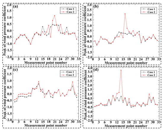
Figure 19.
Maximum value of wind pressure coefficient of cross-section under each wind angle: (a) 0°; (b) 30°; (c) 60°; (d) 90°.
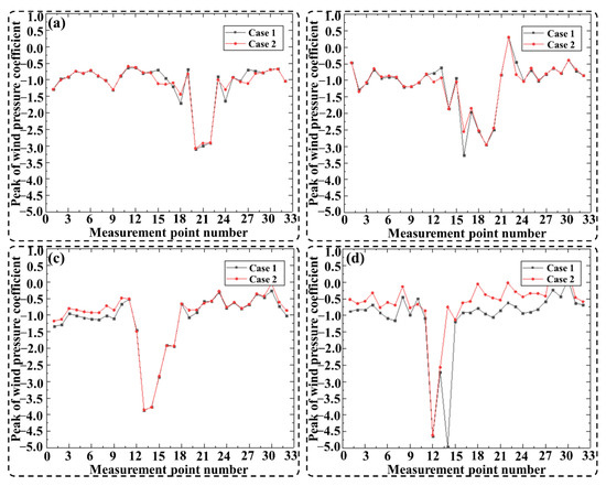
Figure 20.
Minimum value of wind pressure coefficient of cross-section under each wind angle: (a) 0°; (b) 30°; (c) 60°; (d) 90°.
4. Conclusions
This paper adopts a large-eddy simulation method to investigate the extreme wind pressure characteristics on the surface of the open prefabricated spatial grid structures of Evergrande Stadium. The random number cyclic pre-simulation method was applied to the inlet boundary conditions of large-eddy simulation, and its accuracy was verified using the TTU standard model. Taking Evergrande Stadium as an example, the characteristics of wind pressure probability density distribution, the criteria for dividing Gaussian and non-Gaussian regions, different polar calculation methods, and factors influencing the surface polar wind pressure distribution were discussed. The following key conclusions were drawn:
- (1)
- Since the wind pressure time series at most measurement points on the surface of the open prefabricated spatial grid structure does not conform to the Gaussian assumption, the Gaussian distribution is poorly fitted. The GEV distribution and the 3P-gamma distribution perform better. For different measurement points in different regions, the fitting effectiveness of the five common distributions varies. It is necessary to select a suitable distribution function for fitting according to the probability density distribution of wind pressure coefficients at representative measurement points.
- (2)
- The skewness and kurtosis are the criteria for dividing the Gaussian and non-Gaussian regions of this open prefabricated spatial grid structure. The measurement points meeting this criterion are classified in the non-Gaussian region, while the rest belong to the Gaussian region. The delineation results reveal that the Gaussian area on the upper surface of the roof is the largest at a 30° wind angle, and the lower surface is at 60°. Moreover, the Gaussian regions under each wind angle are less than half of the total area of the roof.
- (3)
- The extreme values of wind pressure coefficients obtained by the peak factor method will be underestimated because the probability distribution of wind pressure at numerous measurement points does not conform to the Gaussian distribution. Moreover, the improved peak factor method introduces a non-Gaussian correction term, correcting the accuracy, but its results are still small. The absolute error rates for both range from 17–35%. The modified Hermite method fully considers the non-Gaussian characteristics of the probability distribution of wind pressure, making the average error rate controlled within 13%, with high estimation accuracy.
- (4)
- At a wind angle of 0°, the airflow will be strongly separated at the highest part of the roof in the windward area, resulting in a significant wind suction force due to the saddle-like shape of the roof. In contrast, the phenomenon is not apparent at 90°. After crossing the openings, the airflow separates again on the upper surface of the roof away from the edge of the windward area, so the maximum and minimum value of wind pressure coefficient here at 0° and 90° is small, respectively.
- (5)
- The surface roughness of the roof can influence the extreme-value distribution of the wind pressure coefficient in the open prefabricated spatial grid structure in the local region. Specifically, this factor will decrease the maximum value of the wind pressure coefficient while it has a negligible effect on the distribution of the minimum value.
Author Contributions
G.C.: Conceptualization, Methodology, Validation, Investigation, Data Curation, Visualization, Project administration, Writing—Original Draft, Writing—Review and Editing; Y.H.: Conceptualization, Methodology, Validation, Investigation, Data Curation, Visualization, Project administration, Writing—Original Draft, Writing—Review and Editing; P.W.: Data Curation, Visualization; R.F.: Conceptualization, Resources, Supervision; F.Z.: Data Curation, Visualization. All authors have read and agreed to the published version of the manuscript.
Funding
This research was financially supported by the National Natural Science Foundation of China (Grant number: 5197082474) and Science and Technology Project of Jiangsu Province (Grant number: BY2021099).
Institutional Review Board Statement
Not applicable.
Informed Consent Statement
Not applicable.
Acknowledgments
The authors wish to acknowledge the Key Laboratory of Concrete and Prestressed Concrete Structures of the Ministry of Education, Southeast University. Finally, and most importantly, the authors wish to thank the anonymous reviewers for their thorough evaluations and valuable comments, which have helped improve the paper.
Conflicts of Interest
The authors declare no conflict of interest.
References
- General Administration of Quality Supervision; Inspection and Quarantine of P.R.C; Ministry of Housing and Urban-Rural Development of P.R.C. Load Code for the Design of Building Structures (GB 50009-2012); China Construction Industry Press: Beijing, China, 2012. [Google Scholar]
- Nakamura, O.; Tamura, Y.; Miyashita, K.; Itoh, M. A case study of wind pressure and wind-induced vibration of a large span open-type roof. J. Wind Eng. Ind. Aerodyn. 1994, 52, 237–248. [Google Scholar] [CrossRef]
- Wu, P.; Chen, G.; Feng, R.; He, F. Research on wind load characteristics on the surface of a towering precast television tower with a grid structure based on large eddy simulation. Buildings 2022, 12, 1428. [Google Scholar] [CrossRef]
- Huang, Y.; Yang, J.; Feng, R.; Chen, H. Resistance of cold-formed sorbite stainless steel circular tubes under uniaxial compression. Thin-Walled Struct. 2022, 179, 109739. [Google Scholar] [CrossRef]
- Huang, Y.; Yang, J.; Zhong, C. Flexural performance of assembly integral floor structure voided with steel mesh boxes. J. Build. Eng. 2022, 54, 104693. [Google Scholar] [CrossRef]
- Sun, S.; Niu, Z.; Wang, D.; Zhang, X.; Duo, L.L. Bond behavior of coral aggregate concrete and corroded Cr alloy steel bar. J. Build. Eng. 2022, 61, 105294. [Google Scholar] [CrossRef]
- Jeong, J.; Hussain, F. On the identification of a vortex. J. Fluid Mech. 1995, 285, 69–94. [Google Scholar] [CrossRef]
- Galletti, C.; Mariotti, A.; Siconolfi, L.; Mauri, R.; Brunazzi, E. Numerical investigation of flow regimes in T-shaped micromixers: Benchmark between finite volume and spectral element methods. Can. J. Chem. Eng. 2019, 97, 528–541. [Google Scholar] [CrossRef]
- Dhamankar, N.S.; Blaisdell, G.A.; Lyrintzis, A.S. Overview of turbulent inflow boundary conditions for large-eddy simulations. AIAA J. 2018, 56, 55528. [Google Scholar] [CrossRef]
- Tabor, G.R.; Baba-Ahmadi, M.H. Inlet conditions for large eddy simulation: A review. Comput. Fluids 2010, 39, 553–567. [Google Scholar] [CrossRef]
- Spalart, P.R. Direct simulation of a turbulent boundary layer up to Rθ = 1410. J. Fluid Mech. 1988, 187, 61–98. [Google Scholar] [CrossRef]
- Lund, T.S.; Wu, X.; Squires, K.D. Generation of Turbulent Inflow Data for Spatially-Developing Boundary Layer Simulations. J. Comput. Phys. 1998, 140, 233–258. [Google Scholar] [CrossRef]
- Ferrante, A.; Elghobashi, S.E. A robust method for generating inflow conditions for direct simulations of spatially-developing turbulent boundary layers. J. Comput. Phys. 2004, 198, 372–387. [Google Scholar] [CrossRef]
- Morgan, B.; Larsson, J.; Kawai, S.; Lele, S.K. Improving low-frequency characteristics of recycling/rescaling inflow turbulence generation. AIAA J. 2011, 49, 582–597. [Google Scholar] [CrossRef]
- Wang, T. Large Eddy Simulation of Atmospheric Boundary Layer Flow Based on FLUENT. Ph.D. Thesis, Beijing Jiaotong University, Beijing, China, 2011. [Google Scholar]
- Davenport, A.G. Gust Loading Factors. J. Struct. Div. 1967, 93, 11–34. [Google Scholar] [CrossRef]
- Peterka, J.A.; Cermak, J.E. Wind pressures on buildings—Probability densities. ASCE J. Struct. Div. 1975, 101, 1255–1267. [Google Scholar] [CrossRef]
- Kareem, A.; Zhao, J. Analysis of non-gaussian surge response of tension leg platforms under wind loads. J. Offshore Mech. Arct. Eng. 1994, 116, 137–144. [Google Scholar] [CrossRef]
- Suresh Kumar, K.; Stathopoulos, T. Synthesis of non-Gaussian wind pressure time series on low building roofs. Eng. Struct. 1999, 21, 1086–1100. [Google Scholar] [CrossRef]
- Sadek, F.; Simiu, E. Peak Non-Gaussian Wind Effects for Database-Assisted Low-Rise Building Design. J. Eng. Mech. 2002, 128, 530–539. [Google Scholar] [CrossRef]
- Rice, S.O. Mathematical Analysis of Random Noise. Bell. Syst. Tech. J. 1945, 24, 46–156. [Google Scholar] [CrossRef]
- Grigoriu, M. Crossings of Non-Gaussian Translation Processes. J. Eng. Mech. 1984, 110, 610–620. [Google Scholar] [CrossRef]
- Kasperski, M. Specification of the design wind load-A critical review of code concepts. J. Wind Eng. Ind. Aerodyn. 2009, 97, 335–357. [Google Scholar] [CrossRef]
- Holmes, J.D. Non-gaussian characteristics of wind pressure fluctuations. J. Wind Eng. Ind. Aerodyn. 1981, 7, 103–108. [Google Scholar] [CrossRef]
- Nozawa, K.; Tamura, T. Large eddy simulation of the flow around a low-rise building immersed in a rough-wall turbulent boundary layer. J. Wind Eng. Ind. Aerodyn. 2002, 90, 1151–1162. [Google Scholar] [CrossRef]
- Lettau, H. Note on Aerodynamic Roughness-Parameter Estimation on the Basis of Roughness-Element Description. J. Appl. Meteorol. 1969, 8, 828–832. [Google Scholar] [CrossRef]
- Wooding, R.A.; Bradley, E.F.; Marshall, J.K. Drag due to regular arrays of roughness elements of varying geometry. Bound.-Layer Meteorol. 1973, 5, 285–308. [Google Scholar] [CrossRef]
- Liu, G.; Xuan, J.; Park, S.U. A new method to calculate wind profile parameters of the wind tunnel boundary layer. J. Wind Eng. Ind. Aerodyn. 2003, 91, 1155–1162. [Google Scholar] [CrossRef]
- Yu, Y.; Yang, Y.; Xie, Z. A new inflow turbulence generator for large eddy simulation evaluation of wind effects on a standard high-rise building. Build. Environ. 2018, 138, 300–313. [Google Scholar] [CrossRef]
- Feng, C.; Gu, M.; Zheng, D. Numerical simulation of wind effects on super high-rise buildings considering wind veering with height based on CFD. J. Fluids Struct. 2019, 91, 102715. [Google Scholar] [CrossRef]
- Zhou, L.; Hu, G.; Tse, K.T.; He, X. Twisted-wind effect on the flow field of tall building. J. Wind Eng. Ind. Aerodyn. 2021, 218, 104778. [Google Scholar] [CrossRef]
- Papp, B.; Kristóf, G.; Gromke, C. Application and assessment of a GPU-based LES method for predicting dynamic wind loads on buildings. J. Wind Eng. Ind. Aerodyn. 2021, 217, 104739. [Google Scholar] [CrossRef]
- Yan, B.W.; Li, Q.S. Detached-eddy and large-eddy simulations of wind effects on a high-rise structure. Comput. Fluids 2017, 150, 74–83. [Google Scholar] [CrossRef]
- van Hooff, T.; Blocken, B.; Tominaga, Y. On the accuracy of CFD simulations of cross-ventilation flows for a generic isolated building: Comparison of RANS, LES and experiments. Build. Environ. 2017, 114, 148–165. [Google Scholar] [CrossRef]
- Zhou, X.; Zu, G.; Gu, M. Comparative study of TTU standard model surface wind pressure large eddy simulation and wind tunnel test. Eng. Mech. 2016, 33, 104–110. [Google Scholar]
- Levitan, M.L.; Mehta, K.C. Texas tech field experiments for wind loads part II: Meteorological instrumentation and terrain parameters. J. Wind Eng. Ind. Aerodyn. 1992, 43, 1577–1588. [Google Scholar] [CrossRef]
- Surry, D. Pressure measurements on the Texas tech building: Wind tunnel measurements and comparisons with full scale. J. Wind Eng. Ind. Aerodyn. 1991, 38, 235–247. [Google Scholar] [CrossRef]
- Stathopoulos, T. PDF of wind pressures on low-rise buildings. ASCE J. Struct. Div. 1980, 106, 973–990. [Google Scholar] [CrossRef]
- Pasqualetto, E.; Lunghi, G.; Rocchio, B.; Mariotti, A.; Salvetti, M.V. Experimental characterization of the lateral and near-wake flow for the BARC configuration. Wind Struct. Int. J. 2022, 34, 101–113. [Google Scholar] [CrossRef]
- Perna, R.; Abela, M.; Mameli, M.; Mariotti, A.; Pietrasanta, L.; Marengo, M.; Filippeschi, S. Flow characterization of a pulsating heat pipe through the wavelet analysis of pressure signals. Appl. Therm. Eng. 2020, 171, 115128. [Google Scholar] [CrossRef]
- Li, Z.; Li, C. Non-Gaussian non-stationary wind pressure forecasting based on the improved empirical wavelet transform. J. Wind Eng. Ind. Aerodyn. 2018, 179, 541–557. [Google Scholar] [CrossRef]
- Wickersham, A.J.; Li, X.; Ma, L. Comparison of Fourier, principal component and wavelet analyses for high speed flame measurements. Comput. Phys. Commun. 2014, 185, 1237–1245. [Google Scholar] [CrossRef]
- Sun, Y. Research on Wind Load Characteristics of Large Span Roof Structure. Ph.D. Thesis, Harbin Institute of Technology, Harbin, China, 2007. [Google Scholar]


Disclaimer/Publisher’s Note: The statements, opinions and data contained in all publications are solely those of the individual author(s) and contributor(s) and not of MDPI and/or the editor(s). MDPI and/or the editor(s) disclaim responsibility for any injury to people or property resulting from any ideas, methods, instructions or products referred to in the content. |
© 2022 by the authors. Licensee MDPI, Basel, Switzerland. This article is an open access article distributed under the terms and conditions of the Creative Commons Attribution (CC BY) license (https://creativecommons.org/licenses/by/4.0/).