Abstract
Indonesia is located in a high-seismic-risk region with a significant number of non-engineered houses, which typically have a higher risk during earthquakes. Due to the wide variety of differences even among parameters within one building typology, it is difficult to capture the total risk of the population, as the typical structural engineering approach to understanding fragility involves tedious numerical modeling of individual buildings—which is computationally costly for a large population of buildings. This study uses a statistical learning technique based on Gaussian Process Regression (GPR) to build the family of fragility curves. The current research takes the column height and side length as the input variables, in which a linear analysis is used to calculate the failure probability. The GPR is then utilized to predict the fragility curve and the probability of collapse, given the data evaluated at the finite set of experimental design. The result shows that GPR can predict the fragility curve and the probability of collapse well, efficiently allowing rapid estimation of the population fragility curve and an individual prediction for a single building configuration. Most importantly, GPR also provides the uncertainty band associated with the prediction of the fragility curve, which is crucial information for real-world analysis.
1. Introduction
Indonesia is located in a highly seismic region, and in the past two decades, the region has also experienced numerous large earthquakes (most notably, Aceh in 2004, Padang in 2009, Lombok in 2018, Palu in 2018, etc.) with devastating consequences, whether economic or human lives. Yet, it is well known that earthquakes must not always result in deaths. For example, an analysis of more than 7000 disasters over the past two decades, in which 1.35 million people died, showed that 90% of those deaths occurred in low- and middle-income countries [1], which might be a result of poor mitigation strategies and inadequate building quality.
Indonesia reportedly has a significant number of non-engineered houses, even in the capital city of Jakarta [2], which typically have a higher risk during earthquakes. Non-engineered buildings are spontaneously and informally constructed without any or little intervention by professional engineers [3]. Non-engineered buildings can vary depending on locally available materials or construction methodologies that have permeated a particular region. In this definition, non-engineered buildings can be wooden buildings, masonry, reinforced concrete (RC) frames, adobe structures, etc. However, in the context of Southeast Asia, especially Indonesia, the most prevalent building techniques involve unconfined masonry or RC frames with infilled masonry [4]. Non-engineered buildings also typically do not follow national standards or international design practices and, therefore, might have limited detailing at the connections or between elements [3], making the analysis of their structural behavior more difficult.
In terms of technical characteristics, regional variation in building practices for non-engineered buildings also exists. Indonesia has some significant differences even when compared with other developing countries. The column area is the smallest compared to Nepal, India, Turkey, Peru, Egypt, and Pakistan, with less than 20,000 mm2, almost 50% of the area value of the average of the other countries. The analysis of structural performance in building elements also shows that one of the most-significant issues in non-engineered buildings has been the accuracy in construction practices [5]. A site survey conducted after the 2009 Padang Earthquake indicated that damages to non-engineered RC frame structures in Padang showed crushing of column ends, which led to complete collapses of stories [6]; this failure mechanism is typically due to inadequate detailing.
In this study, we focus on analyzing non-engineered RC frames, which are becoming widespread in semi-urban and rural areas in various countries. Non-engineered RC frames that use isolated columns in parallel with load-bearing walls for supporting long internal beams or those in verandahs and porches are becoming quite common. In most cases, such constructions suffer from deficiencies from the seismic viewpoint since no consideration is given to the effect of lateral seismic loads. The connection details are usually such that no moment carrying capacity can be relied upon. Beams simply rest on the columns and are primarily held in position through friction. Typical damages and collapses of RC building include [3] sliding of roofs off supports, falling of infill walls, crushing of column ends and virtual hinging, the short column effect, diagonal cracking, diagonal cracking in columns, diagonal cracking of column–beam joints, pulling out of reinforcing bars, and collapse of gable frames (see Figure 1).

Figure 1.
From left to right: (a) crushing of the concrete at the end of columns from the 2007 West Sumatra Earthquake, which may lead to the complete collapse of a story, as seen in this (b) RC collapsed building during the 2005 Northern Pakistan Earthquake (source: Arya et al. [3]), and (c) short column formation caused by ribbon windows in residential buildings in Turkey (source: Cogurcu [7]).
Due to the wide variety of differences even among parameters within one building typology, understanding the total risk of the population is a challenging task. The typical structural engineering approach to understanding fragility involves tedious numerical modeling of individual buildings—which is computationally costly for a large population of structures. Most risk assessment, therefore, simplifies the process by either only screening building using rapid visual assessment and then complementing the data with a more detailed structural analysis only for a selected group or structure that is deemed to have a higher risk or is an archetype building [8,9,10] or by using the typology approach (assessed by rapid visual screening) and, then, assigning an estimated fragility for a given building typology (EMS1998 [11]). However, neither method can describe the differences in behavior among individual buildings. Another problem is that data is scarce for a large portion of the world’s most vulnerable seismic countries. Such a condition makes risk assessments depend largely on building typology assumptions that are uniform for the whole region and whose fragility is created based on earthquake data from specific regions only.
In order to estimate population risk better, it is necessary to build fragility curves for multiple combinations of parameters. However, obtaining a complete family of fragility curves with pure random sampling is computationally infeasible. One potential technique is to deploy a surrogate model [12], accompanied by the respective uncertainty, to predict the fragility curves for a large combination of parameters. This, in turn, will be of great assistance since no further simulation is needed to evaluate a specific combination. A surrogate model is essentially an approximation model that tries to mimic the relationship between input variables/parameters and the output of interest [13]. Formally, a surrogate model is an inexpensive approximation of the original function, which is constructed by using a finite set of experimental designs. Such a strategy allows subsequent tasks (e.g., optimization or uncertainty analysis) to be efficiently performed by calling the surrogate model instead of the actual simulation, significantly reducing the computational burden. Approximation models essentially allow rapid prediction of family fragility curves, which helps provide information on the seismic risk assessment of a large population. If the variation of the parameter distribution within a given population is known, a closer and more well-informed population risk can be calculated. Surrogate models have been applied to estimate seismic responses in some previous papers. For example, Yan et al. [14] developed a procedure based on surrogate models to estimate mean fragility curves given uncertainties in the structural parameters. Esteghamati and Flint developed a surrogate model framework to estimate seismic responses and also performed a global sensitivity analysis to identify the most important input variables [15]. Recently, Anwar and Dong deployed Gaussian Process Regression (GPR) to assess community building portfolios and performed risk assessment using utility theory [16].
This paper uses a machine learning technique based on GPR to build the family of fragility curves [17]. The GPR model is constructed using an experimental design evaluated at several combinations of the building parameters. After the GPR model has been built, it can be conveniently used to predict the fragility curves for any untested combinations. The GPR model essentially provides a rapid prediction model for estimating the family of fragility curves, which is computationally infeasible if we only rely on simulations. Gentile and Galasso first studied the utilization of GPR for seismic fragility assessment of building portfolios [18]. While Gentile and Galasso focused on the predictive accuracy of GPR, in this paper, we explore other capabilities of GPR to provide the uncertainty associated with the prediction. In contrast with the majority of other machine learning models such as support vector machine or deep neural networks, the added value of GPR is that it also provides the uncertainty of the prediction, which is especially important for users to assess the confidence of the predicted fragility curve. The uncertainty quantification is important because a surrogate model is essentially an approximation and should be accompanied by the uncertainty estimate. In addition, this paper explores the constructed GPR model to analyze the impact of changing building parameters on the fragility curve. Such knowledge is especially important for engineers in parametric and sensitivity studies, in which this paper shows that GPR is of great assistance in aiding such endeavors. Finally, another originality of this paper is that we utilize GPR for seismic risk assessment; that is, we predict the Probability of Collapse (PoC) for a given hazard in a particular region. GPR itself has been previously used in several structural engineering applications, for example reduced-order modeling in nonlinear structural mechanics [19], structural reliability analysis [20,21], structural optimization [22], parameter identification [23], finite-element model updating [24], and uncertainty analysis [25]. Outside structural engineering, but still in the domain of civil engineering, GPR has been used in the aeroelastic prediction of bridge structure [26] and aerodynamic optimization of civil structures [27].
The paper is organized as follows.
Section 2 describes the specific characteristics of non-engineered residential houses in Indonesia. These characteristics provide a justification of the range of investigated structural member dimensions, failure mode, and type of analysis employed in the subsequent sections. In Section 3, the data and methodology used in this paper are presented. Here, the general methodology is given by highlighting the strengths and limitations of the processes in each phase. In Section 4, the results and discussions are given. Finally, in Section 5, the conclusion and future works are presented.
2. Overview of Non-Engineered Residential Houses and Earthquakes in Indonesia
The typical characteristics of non-engineered residential houses in Indonesia include: (1) many openings in the wall to accommodate windows and doors, which will weaken the wall (see Figure 2); (2) no ties (proper anchorage) between the masonry wall and the surrounding frames, meaning no significant strength and stiffness contribution is provided by the masonry walls (see Figure 3a); (3) a small column size in the range of about 15–25 cm (even generally smaller than the typical beam sizes), which does not fulfil the strong column–weak beam criterion (see Figure 3b,c); (4) no to minimum confinement (sparse ties > 20 cm), resulting in no ductility in the structure (see Figure 3b,c).
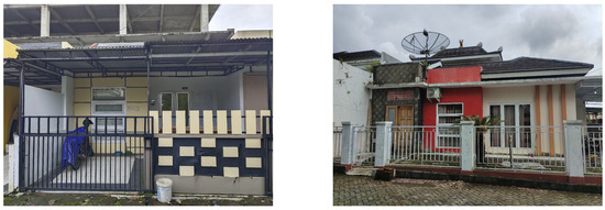
Figure 2.
Typical non-engineered houses in Indonesia.
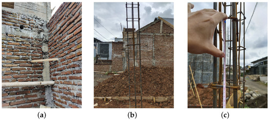
Figure 3.
Field data of an on-going construction of a non-engineered residential buildings (a) No anchorage between the masonry wall and frame. (b) Small column size. (c) No to minimum confinement.
The above trends within non-engineered residential houses result in typical failure modes as observed in most earthquakes including the recent one in Cianjur, West Java Indonesia (November 2022). Shown in Figure 4 are documentations from a recent field survey in Cianjur. Despite the relatively not-so-large magnitude of the corresponding earthquake (5.6 Mw), the death toll and structural destruction experienced, especially to non-engineered housings in this particular area, were sizable. The typical damages include:
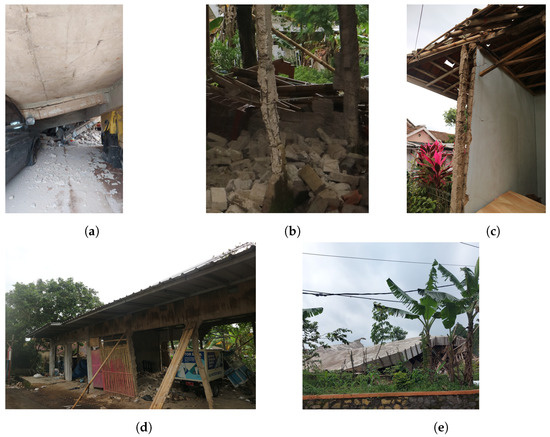
Figure 4.
Typical failure mechanisms of non-engineered residential buildings during the Cianjur Earthquake 2022. (a) Soft-story failure with strong beam–weak column. (b) No to minimum confinement. (c) No connection between the column and walls. (d) Column failure. (e) Soft-story with pancaking mechanism.
- Typically soft-story failures where the column is weaker than the beam (see Figure 4a,d,e);
- No to minimum confinement (sparse ties), resulting in no ductility in the structure (see Figure 4b);
- Masonry walls that are not well anchored and confined to the frames, making the walls have a minimum contribution towards structural integrity and making even most confined masonry behave like a bare-frame structure (see Figure 4c).
The majority of the collapse patterns that we observed were clearly caused by the failure of the column member, which resulted in a soft-story (pancaking) mechanism (see Figure 4d,e). Therefore, in this study, we focus on estimating the behavior of such structures, which are mostly dominated by column failure.
3. Data and Methodology
This section is organized as follows: firstly, the general methodology is presented, then a more detailed explanation for each of the phases is given.
3.1. General Methodology
This research was performed in three phases, where the first and second phase focus on the structural engineering part of the problem, starting with structural modeling and simulation (Phase I), then continuing to creating the fragility curves dataset that will be used for GPR (Phase II). Finally, the third phase presents the process of predicting the seismic fragility of non-engineered buildings (see Figure 5 for clarity).
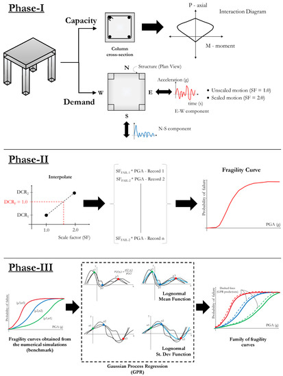
Figure 5.
An illustration of the general methodology adopted in this study. Overall, the methodology can be divided into three phases: (1) the definition of the structural models (resistance) and the application of ground motion records (demand); (2) the creation of numerical fragility curves; (3) the application of Gaussian Process Regression(GPR).
In Phase I, a structural model is built based on a predefined column height and dimension, producing different axial–moment interaction capacities for each case. It is important to note that, based on the previous study on the behavior of non-engineered residential buildings in Bandung [28] and additional observations elaborated in Section 2, it is assumed here that the capacity of the structure is solely governed by the failure of the column as the predefined collapse limit state used in this analysis. Other types of failure modes, such as joint shear failure or beam failure, were not considered. The demand parameters are represented by suites of ground motions consisting of acceleration time history in major and minor directions with wide variations of Peak Ground Acceleration (PGA) and intensity to capture the randomness of the seismic load (see Table 1).

Table 1.
The list of ground motions used in this study.
In Phase II, the seismic fragility of the structural models is investigated by up-scaling and interpolating the suite of ground motions to identify the exact level of PGA where the collapse limit state is reached (demand-capacity ratio = 1) for each case by means of Linear Time History Analysis (LTHA). Then, by assuming a lognormal distribution, both the Probability Density Function (PDF) and Cumulative Density Function (CDF) can be obtained. This process is then repeated for every structural model with a different column height and dimension set to produce the benchmark fragility curves for GPR.
In Phase III, each predefined column height and dimension combination yields the corresponding fragility curve, as defined by the mean and standard deviation of the lognormal distribution. A GPR model is constructed by using the dataset evaluated at specific combinations of column height and dimension. Formally, we collect the experimental design and the corresponding responses to build a GPR model. There are two outputs from a GPR model: the prediction and the uncertainty estimate. Because we aimed to predict fragility curves, there are two GPR models, each for predicting the mean and the standard deviation of the lognormal distribution, respectively. For an arbitrary point, a single fragility curve can be predicted using the lognormal distribution’s predicted mean and standard deviation. The uncertainty estimate of the fragility curve is then constructed using Monte Carlo simulation applied to the surrogate model.
3.2. Phase I: Structural Modeling and Simulation
3.2.1. Field Data Collection
Field data were obtained to construct a typical public housing structure from in-depth interviews with local contractors in Bandung, Indonesia, which focus on building houses/simple structures for the lower to middle class groups [28]. First, the local contractors were provided with a case of a residential building with a floor area equal to that stated by the regulations for Public Housing by the Indonesian Ministry of Public Works and Public Housing. The local contractors were then asked to explain how they would construct this structure.
The structural dimensions obtained from field data were within the range of 30,000 mm2 for the beam and 22,500 mm2 for the column. The hoops’ spacing was somewhere within the range of 250 mm to 300 mm. Kusumastuti [29] stated that the common practice of the concrete mixture for residential houses with the ratio of 1:2:3 for the volume of cement, sand, and coarse aggregate, respectively, produces concrete with a compressive strength of approximately 17 MPa. Field data also show an average rebar size of around 10 mm for longitudinal rebar and 6 mm for hoops with a lower range yield strength of 240 MPa. With these collected data of the dimensions and materials, a typical single-story public housing structure was constructed (see Figure 6a) [28]. Previous research showed that the failure mechanism occurs at the column, which has the highest bending moment compared to other structural elements in the event of an earthquake, followed by beams [28]. Besides, as shown from the documentations of the collapsed houses from the recent earthquake in Cianjur (refer to Section 2), soft-story collapse is typically caused by column failure, hence justifying the assumption.
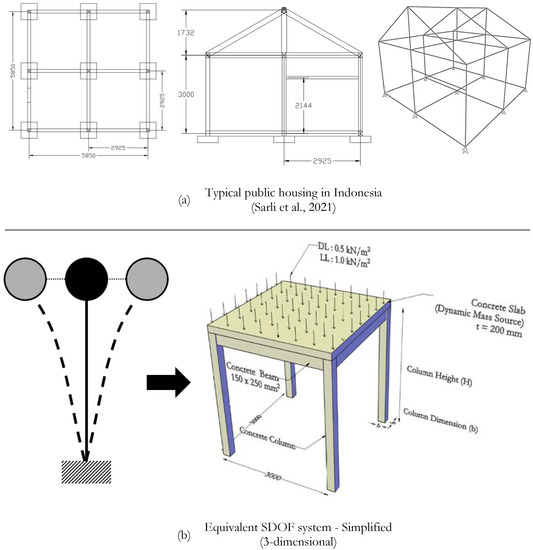
Figure 6.
Simplified numerical model used in the present simulation ([28]).
3.2.2. Numerical Model
In this study, Linear Time History Analysis (LTHA) was performed rather than the more typical Nonlinear Time History Analysis (NLTHA). The use of LTHA versus NLTHA can be dictated by the structural system that is being assessed. It is true that NLTHA typically produces a more realistic assessment for engineered structures governed by deformation-controlled behavior where sufficient ductility allows such structures to reach their “plastic” ultimate resistance. However, as this study focused on assessing the seismic performance of non-engineered housings, NLTHA might not be entirely suitable. Observation from the field visit showed that typical non-engineered housing structures in Indonesia are not designed and built with appropriate seismic detailing. Besides, the design capacity concept is overlooked as we have observed from the fact that, generally, column elements are weaker than the beams. The masonry walls that are supposed to provide a lateral-resisting mechanism are built without proper anchoring to the RC frame, and many large openings are typically created in these walls to accommodate windows and doors (the masonry walls are not effectively confined by the surrounding RC frames). Analyzing these structures with NLTHA would be unsuitable and even unsafe, as their actual behavior is very brittle and better represented by LTHA, where failures can be checked based on the demand capacity ratio, as typically adopted for force-controlled behavior.
The typical public housing structure, as obtained from field data (see Figure 6a), was then constructed as a simplified numerical model equivalent to an SDOF structural system. The simplified model shown in Figure 6b was created to mimic the main characteristics of the typical public housing model, yet with less computation time to perform the required time history analysis. The columns of the simplified model were assumed to be fully fixed on the ground level. The concrete compressive strength (fc’) and the rebar yield stress (fy) were taken as 15 MPa and 240 MPa, respectively, which were adapted from the commonly used material strength in residential houses based on previous field data. Two rebars of 13 mm in diameter were taken as the top and bottom reinforcement of the beam.
Ideally, the numerical model shall include the contribution of the infill masonry walls to the structure’s lateral stiffness, strength, and ductility. However, the actual behavior of the infilled frame structures is often difficult to predict due to its dependency on the construction quality of the connection system and its detailing. Furthermore, as described in Section 2 earlier, masonry walls in typical non-engineered housing structures in Indonesia are not properly anchored (with ties) to the surrounding frames. Thus, to provide a conservative estimate, the infill walls in this study were treated only as nonstructural components in the analysis. Consequently, the walls contribute to the total weight of the building, but not to the strength and stiffness of the structure. Nonstructural components are defined as superimposed dead loads acting on the structural frames and slab. The considered seismic mass includes a load combination of 1.1*(1.0 dead load + 0.25 live load) in accordance with ASCE 41 [30] for linear time history analysis.
Two main building parameters were investigated: the column height and the dimension. Square-shaped columns varying in size from 150 × 150 mm2 to 400 × 400 mm2 in increments of 50 mm on each side with reinforcement proportions of approximately 1% and the column height varying from 2000 mm to 4000 mm in increments of 500 mm were used in the model, as shown in Figure 7. The column size and height median value were based on the dimensions collected from the field study (interview with local contractors). The interaction diagram of the column member was calculated based on the column reinforcement by assuming the concrete as unconfined due to the sparse hoops/ties. A total of 30 structural models with evenly distributed parameters from the range of interest were constructed (see Figure 7, top left, for a detailed model description). An additional set of 4 models with random values within the range of interest were used to check the accuracy of the GPR model.
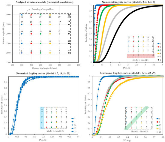
Figure 7.
Design of the experiment and simulated numerical fragility curves.
3.2.3. Ground Motion Selection
To simulate the earthquake magnitude acting on a simple structure, records of past earthquake events were collected and converted to numerical data suitable for structural analysis. The ground motions for Bandung, Indonesia, include acceleration versus time data subjected to the fixed end support of the simplified model. These data are based on the selected pre-recorded ground motion. As currently Indonesia does not have its own ground motion database, the Ground Motions (GMs) were selected from the available PEER database. Then, the hazard deaggregation process was performed by considering all possible Indonesian seismic events to determine the controlling M and R variables that will give the biggest hazard contribution to the investigated site. The GMs from the PEER database with M and R within the range of these controlling values were then selected to ensure that the the seismic hazard of the site was closely represented. These process were considered as the most-optimum (available) scientific variables that can be relied on, as stated in the introductory report related to the new seismic hazard map of Indonesia by PuSGeN [31]. Concerning the tectonic environment, earthquakes in Indonesia are dominated by either the strike–slip or subduction earthquake mechanism. In particular, Bandung (which is the main investigated region in this study) is surrounded by several active faults. This was the main motivation in selecting the strike–slip mechanism as the majority of the adopted ground motion records (6 out of 11 GMs).
The Indonesian code for seismic-resistance building (based on Indonesian National Standard: SNI 1726) specifies that at least 11 pairs of ground motions shall be used for any location. In addition, they shall include two horizontal orthogonal ground motions consistent with the tectonic characteristics that control the site’s spectral target. The seismic deaggregation hazard map developed by Asrurifak [32] through probabilistic analysis was used to determine the seismic characteristics (magnitude and radius of interest) of Bandung. Then, the suites of pre-recorded ground motion were selected based on the magnitude and radius of interest. These suites consist of a mean-source magnitude (M) ranging between 6.2 to 6.6 and a mean-source distance (R) ranging between 20 km to 30 km for Bandung with a 2% probability of exceedance in 50 years (2475-year return period). Lastly, as the soil condition might also influence the ground motion characteristics, the soil site class presented by Sari [33] was used. It was observed that soft soil with a low shear wave velocity () covers most of the center and eastern part of Bandung, while stiff and very dense soil with ranging from 190 m/s to more than 370 m/s is found in the western part. Thus, a broad assumption about the soil condition of the Bandung area was made, in which it ranges between very dense soil to soft soil ( between 175 m/s and 700 m/s). The metadata and spectra are then defined as acceleration-versus-time loads in two orthogonal directions (see Table 1).
It is important to note that, besides the tectonic environment, Magnitude (M), and distance (R), it is generally acknowledged that other factors may also influence the ground motion characteristics of a particular site, including the soil condition. Unfortunately, these other parameters were not specifically explored during the ground motion selection process adopted in the present study due to the unavailable soil data about the investigated site. Still, this phenomenon will be further investigated in future studies.
3.3. Phase II: Numerical Fragility Calculation
3.3.1. Fragility Curve Generation
A fragility curve specifies a structure’s probability of collapse as a function of some ground motion Intensity Measures (IMs). There are three common approaches to collect the data for estimating a fragility function, which are the cloud approach, IDA approach, and Multiple Strip Analysis (MSA) approach, and the major difference between the three approaches is the ground motion selection ([34]). The cloud approach adopts the scattered earthquake motions for linear regression in the logarithmic coordinates. IDA adopts a suite of ground motions that is gradually scaled-up to find the IM level at which individual ground motions cause corresponding structural collapses [35,36,37]. MSA is performed at a specified set of IM levels, each of which has a unique ground motion set [35,38]. The main disparity between the MSA and IDA is that the relationship between the IM and the engineering demand parameter points at different IM levels in the MSA approach not able to be directly linked to the curves as those in the IDA approach ([39]). In this study, the IDA approach was chosen because it provides the whole demand history from the initial elastic stage to the total destruction stage under the increased intensity measures. Besides, since linear time history analysis was adopted in this study (as described in Section 3.2.2), scaling the ground motions from their original state to the intensity level that causes structural collapse is straightforward. Although there are questions about IDA’s representativeness of real earthquake occurrences as it scales the same ground motions up to extreme IM levels [35], previous research [40] has shown that IDA can produce effective fragility estimates even when identical ground motions are consistently used at all IM levels. IDA is also considered as the more-promising approach from the perspective of macro evaluations [36], making it more suitable for our study’s objectives.
Another important discussion is the selection of the Intensity Measure (IM) to be considered in the building of a fragility curve. The most traditionally employed IMs are Peak Ground Acceleration (PGA) and Peak Ground Velocity (PGV), where both are directly available from the measuring station (without any further post-processing). These IMs, although having been criticized for not being able to fully capture the dispersion of the predictions, have undesirable traits relating to inefficiency, sensitivity to scaling, and dependence on other ground motion parameters [41] and are widely employed for the seismic fragility assessment of infrastructures. One of the main reasons is because they are preferred for the availability of national hazard information [42]. Additionally, in the case when the hazard at a site uses a different IM than the fragility formulation, the “conversion” process to obtain the required IM can be quite cumbersome and not straightforward [43]. A more recent study suggests that different IMs shall be adopted for different purposes or objectives [44]. The study recently conducted by Nguyen et al. [44] investigated 20 different IMs for evaluating seismic performances and producing fragility functions of the Reactor Containment Building (RCB). Some statistical operations were employed to determine the coefficient of determination, dispersion (standard deviation), practicality, and proficiency of the correlation between the investigated IMs and the seismic performance of the structure. The study found that the optimal IMs (strongly related) are spectral acceleration, effective peak acceleration, peak ground acceleration, A95, and sustained maximum acceleration, whereas the weakly related IMs include the peak ground displacement, root mean square of displacement, specific energy density, root mean square of velocity, peak ground velocity, Housner intensity, velocity spectrum intensity, and sustained maximum velocity. The present study conducted by the authors employed a single IM, which is the PGA. The main reason justifying this decision is because the vast majority of the available hazard information in Indonesia (the investigated region) is expressed in terms of PGA. Thus, selecting PGA as the main IM was deemed suitable to accommodate the long-term goal of this study, which aims to integrate the estimated fragility curve with the hazard map to obtain the risk map of Indonesia.
It is also important to note that the other more widely used IM, Sa(T1), is observed to be more closely related to inelastic demand than PGA for structures with fundamental periods close to 1 s [15,45,46]. A similar observation was made by Giovenale et al. for SDOF systems with varying ductility and hysteretic behavior [47]. However, it has been demonstrated that Sa(T1) is not a good IM when several modes of response dominate the total dynamic behavior of a structure [48]. Grigoriu argued that, since spectral accelerations and maximum demands are derived from different processes with different frequency bands, they are weakly correlated for linear multiple-degree-of-freedom (MDOF) systems with more than one contributing mode [49]. O’Reilly [41] observed that, in non-ductile infilled RC frame structures, Sa(T1) gives optimal results for IMs at lower intensities, but runs into difficulty once the infill panels collapse and a non-ductile mechanism forms. Hence, as this study observed a structure with limited inelastic ability and non-ductile behavior, PGA was considered as the more suitable choice.
Numerical fragility calculation was carried out through a probabilistic approach to address the uncertainties and randomness of the variables in structural components of structures subjected to earthquakes. Fragility calculation was preceded by numerical model simulation, which can be performed through structural analysis. Through a series of analysis results, the statistical parameters were calculated to construct the fragility curve, which represents the vulnerability characteristic of the structure regarding a seismic event. Specifically, in this study, the LTHA was used to provide the Peak Ground Acceleration (PGA) level at which the structure fails. The elastic approach through LTHA was deemed relevant for the simplified model due to the insignificant ductility of structural components provided by the sparse hoops and poor construction method, thus limiting the development of the inelastic behavior. A conservative and logical assumption was also made about the terminating condition of analysis, where the failure of the simplified model is governed by the first component exceeding capacity (Demand-Capacity Ratio (DCR) = 1).
To obtain the sets of PGA data for fragility calculation in this study, two analyses were performed using the unscaled ground motion (Scale Factor (SF) = 1.0) and the amplified ground motion (SF = 2.0) for each pair of records. Then, the structure’s Demand-Capacity Ratio (DCR) was calculated, providing the DCR for unscaled and amplified records. Then, a simple linear interpolation was performed to obtain the Scale Factor (SF) value, which gives a DCR equal to 1.0. This process was repeated for each ground motion record, and the statistical parameters from the set of PGA data were calculated for each set of column height and dimension.
A lognormal distribution was assumed to construct the Probability Density Function (PDF) and Cumulative Density Function (CDF). The fragility curves in a lognormal distribution were formed due to the record-to-record variation analysis method, with the one-time history yielding exactly one PGA datum, resulting in a unique variation for each case. The fragility function formula to construct the fragility curves is defined as follows [50]:
where represents the PGA resistance level and represents the standard deviation of the distribution. In this study case, the standard deviations only account for the uncertainties in the PGA resistance, while neglecting deviations on the structural restraint and the variability of the materials due to the nature of the small and simple structures. The initial 30 structural models were simulated by LTHA to construct the benchmark fragility curves as the dataset for GPR. Furthermore, the additional set of four random combinations of column height and dimension was used to validate the result of the GP regression (see Figure 7). In addition to checking the suitability of the chosen IM (PGA), additional analyses were also conducted to investigate the dispersion when employing other widely used IMs, that is Sa(T1); the comparison was performed in terms of: (1) fragility functions (CDFs); (2) the coefficient of variation of six chosen structural models (ranging from the shortest to the longest natural period: 0.06–0.6 s).
Overall, the resulting fragility functions (CDFs) (see Figure 8) using the two IMs were sufficiently close for the two models with the shortest natural period (see Models 6 and 14 with T1 < 0.15 s). Still, a more significant deviation could be observed for the models with a longer natural period. The closeness of the two IMs can be potentially explained by the fact that the nature of the investigated structures in this study was that they were all low-rise buildings with a natural period below 0.6. Consequently, the spectral acceleration considering the first mode of vibration, Sa(T1), was not so different from PGA. This is consistent with Yakut and Yılmaz’s [51] observation that, for RC frames with a period between 0.2 s and 0.5 s, PGA gives efficient results.
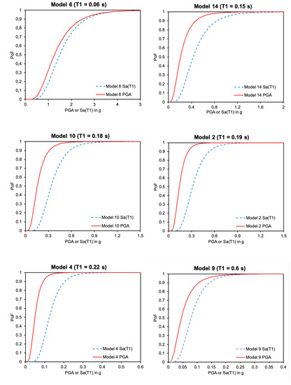
Figure 8.
Fragility curve comparison of the models using Sa(T1) and PGA at different T1 values.
For the dispersion (CoV) obtained using the two IMs for all six models (shown in Figure 9), Sa(T1) generally produces better results with slightly smaller dispersion than PGA. Nevertheless, the two produce relatively large scatters. Therefore, the authors are cautious in stating the general applicability of the results since the range of the investigated structures in this particular study was rather narrow in terms of fundamental period variations. IM and GM selection remain structure and site-specific. No available IM is sufficient in an absolute sense: careful GM selection is needed to account for hazard characteristics that are not represented using the selected IM. GM selection methods must also be chosen in conjunction with the structural response analysis procedure.
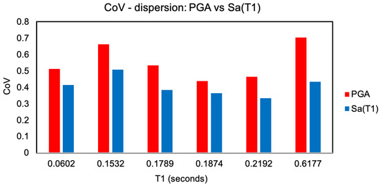
Figure 9.
Coefficient of variation of six chosen structural models (ranging from the shortest to the longest natural period: 0.06–0.6 s) when employing PGA vs. Sa(T1) as the considered Intensity Measure.
3.3.2. Simplified Model Validation
To verify the adequacy of the simplified SDOF (numerical) model in representing the actual behavior of the typical public housing construction, the fragility curves of both structures were constructed based on the above methodology. Figure 10 shows the resulting (numerical) fragility curves of the two structures (actual versus simplified) when subjected to the same set of recorded ground motions. It can be clearly observed from Figure 10 that the two fragility curves are in excellent agreement, which justifies the applicability of the simplified SDOF model. Thus, this SDOF model was consistently employed for all analyses reported in the following sections.
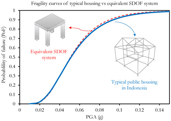
Figure 10.
Numerical fragility curves of the two structures (actual versus simplified) when subjected to the same set of recorded ground motions.
3.4. PHASE III: Gaussian Process Regression
3.4.1. Definition of Gaussian Process Regression
In this paper, we used GPR to construct the model for estimating the parameters of the lognormal distribution. Let us denote the mean and the standard deviation of the fragility curve as and , respectively. The model was constructed by using data at a finite set of sampling points, in which each point corresponds to one specific combination of and . We constructed two models, one for estimating and one for . Any surrogate model can be used for this purpose; however, the model needs to be carefully selected to avoid less accurate approximations. We selected GPR due to its flexibility and advantages over other models, such as support vector regression or polynomial regression. Arguably, the primary advantage of GPR is that it provides not just the prediction, but also the associated uncertainty, which is important for providing the confidence interval to analysts. GPR is also suitable for nonlinear functions, which is accomplished through kernel functions.
The goal of GPR is essentially to construct an approximation model , where is the vector of input variables and m is the dimensionality of the input. Notice that can be any black-box function, in which we want to predict the output given the input. The data that we need to construct a GPR model is evaluated on a finite set of experimental design , where n is the size of the experimental design, with the corresponding vector of responses .
GPR constructs a model as a realization of stochastic process as follows:
where is the mean function and Z is a zero-mean stochastic (Gaussian) process. The responses between two different points, and , are correlated through the kernel function , where is the vector of length scales. This paper used the Gaussian kernel to model the similarities between the responses, which reads as
where a multidimensional Gaussian kernel function is constructed by the product of its one-dimensional counterparts. To build a GPR model, one needs to construct a correlation matrix , where its component defined as where for , is the regression factor, and is the Kronecker delta, where if and 0 otherwise. Similarly, one can also build a correlation vector for any arbitrary point , where its j-th component is , where for . The GPR prediction then reads as
where is a vector of ones of size . Notice that Equation (4) is the mean of the posterior distribution, with the associated uncertainty estimate calculated as follows:
where is the GP variance (i.e., the signal variance).
It is necessary to tune the vector of the length scale to create a model that is optimal in a certain sense. In this paper, the vector of the length scale, the constant mean, and the GP variance were tuned to maximize the likelihood function, described as follows:
where is the vector of the hyperparameters. Using the maximum likelihood principle, the constant mean is analytically estimated as follows:
while the GP variance should be optimized together with the other hyperparameters since no analytical formulation exists. In this paper, we used the covariance matrix adaptation evolution strategy (CMA-ES) [52] to maximize the likelihood function by finding the best combination of hyperparameters.
The posterior probability distribution at any arbitrary point can then be written as:
Figure 11 shows how GPR can be used to create a surrogate model for a one-dimensional Forrester function [12]. Shown in Figure 11a are the true function (), a set of sampling points consisting of seven samples (), the prediction from GP (, which is the mean of the posterior distribution), and the uncertainty estimate (). The uncertainty estimate is critical since it gives users confidence in the predictions’ accuracy. It can be seen that the uncertainty is intuitively smaller at the location where more sampling points are available (i.e., at ). The GPR prediction is sufficiently accurate since it is close to the true function. Shown in Figure 11b are examples of realizations (sample paths) from the posterior distributions to illustrate how the uncertainty estimates were obtained. Notice that only the standard deviation is needed, not every single realization, which is infinite in number.
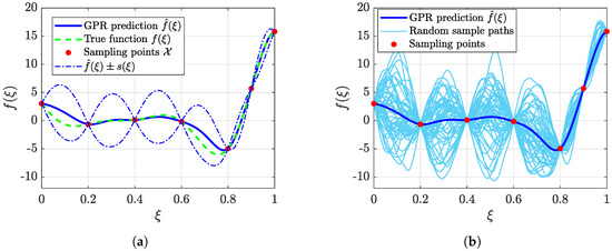
Figure 11.
A demonstration of how GPR approximates the one-dimensional Forrester function. (a) GPR prediction. (b) Random sample paths.
3.4.2. Deploying Gaussian Process Regression
Our GPR model takes the mean and standard deviation of the lognormal distribution (i.e., and ) as inputs (two separate GPR models). The predicted lognormal distribution parameters are then used to build the fragility curve. No further simulation is needed since the fragility curve is predicted based on the data. Later on, we used the probability of collapse to build the GPR model to estimate the risk of a specific hazard. The dataset is based on the full-factorial design, with 6 and 5 samples for spanning the column dimension and column height, respectively. The column dimension and weight were assumed to be uniformly distributed as follows: b∼ and H∼. From this procedure, we obtained the regression model for and , namely and , respectively (notice that we do not write the dependency on and for shorter notations). Notice that other sampling methods, such as Latin hypercube sampling, are more suitable for higher input dimensions. We selected a full-factorial design since it suits our current problem, which has two input variables.
The uncertainty information from the GPR model is crucial in assessing the predicted fragility curve. Providing such information is essential because there are always uncertainties associated with a prediction. Fortunately, the probabilistic nature of GPR allows us to provide the uncertainties in the predicted fragility curve. It is worth mentioning that the uncertainty from GPR corresponds to the prediction of the mean and the standard deviation of the lognormal distribution. Thus, we propagated the uncertainty of the mean and the standard deviation to the fragility curve by random sampling. The uncertainty can be associated with either a single prediction (i.e., one combination of the input parameters) or the whole population. Notice that the population space consists of all combinations of column length and height.
Let us first discuss the uncertainty of a single prediction, for example at . To obtain the confidence interval for a single prediction of the fragility curve at , we performed a large amount of sampling from and to obtain the family of fragility curves. To be exact, we used a Monte Carlo simulation with 100,000 samples, in which the confidence interval is then constructed by calculating the percentiles of this set of fragility curves. The most common level is 90%; thus, we calculated the 5th and 95th percentiles to obtain the confidence interval for a single prediction. The first type of confidence interval is useful for assessing the fragility curve for a single building.
To assess the distribution of the population fragility curves as defined by the distribution of the inputs, we used a Monte Carlo simulation by random sampling in the input space of b and H (both were assumed to be uniformly distributed) to build the population fragility curves. It is worth noting that the predicted family of curves is also subjected to uncertainty in the GPR prediction. Thus, for a single realization of , the realization of and is also sampled from and .
4. Results and Discussions
4.1. Predicted Fragility Curves and Validation
The GPR plots for the mean and the standard deviation of the lognormal distribution are shown in Figure 12. However, before discussing the result, we checked the validity of the constructed GPR models by comparing the simulated and predicted fragility curves with the test set. The evaluation of the model is necessary to verify its usability. It is worth noting that the information from the two separate GPR models was combined into predictions of the fragility curve. Thus, for a specific combination of b and H, we estimated the fragility curve based on the lognormal distribution’s predicted mean and standard deviation. As mentioned earlier, one virtue of a GPR model is that it also provides the uncertainty associated with the prediction. The uncertainty from the GPR model (i.e., ) is only applicable to the original output, which comprises the mean and standard deviation of the fragility curve. Therefore, an additional procedure is required to estimate the uncertainty in the predicted fragility curve.
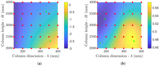
Figure 12.
Plots of GPR predictions for the mean and standard deviation of the lognormal distribution from the fragility curve. Filled dots and diamonds are the sampling and validation points, respectively. (a) Mean of lognormal distribution. (b) Standard deviation of lognormal distribution.
We constructed the uncertainty in the fragility curve by sampling a large number of realizations from the normal distributions of the predictions from the two GPR models. In other words, for a single combination of b and H, we created a large number of realizations of fragility curves whose parameters were predicted from the GPR models (remember that GPR yields the prediction in the form of distributions, not a single value). The confidence interval can then be calculated simply by taking the percentiles of the multiple realizations of the fragility curves. We then verified the predictions by using a separate test set consisting of four samples that were not used in the training phase of the GPR model: (1) mm, mm, (2) mm, mm, (3) mm, mm, and (4) mm, mm. These validation points’ locations were arranged so that they were located far from each other (see Figure 12).
The steps to verify the accuracy of our model were as follows. First, using the constructed GPR model, we calculated the predicted mean and standard deviation of the lognormal distribution (i.e., and , respectively, for the four test points). Next, we sampled 100,000 realizations from and (i.e., the posterior distribution of GPR) for each of the four test points. Notice that each of these 100,000 samples corresponds to a single fragility curve, that is a single realization from the prior distribution of the predicted fragility curve. The 90% confidence interval can then be obtained from these 100,000 samples. Next, we compared the mean predicted fragility curve and the corresponding confidence interval to the actual simulation. The prediction can be considered accurate and reliable if (1) it is close to the actual simulation and (2) the confidence intervals are sufficiently narrow.
It is important to remark that the database of ground motions adopted in the present study was relatively small (i.e., only fulfilling the lower bound of typical prescribed seismic provisions). Consequently, the Record-To-Record (RTR) variation might be less pronounced, affecting the GPR method’s resulting predictions. It is possible that, when a larger database of ground motions is used, the GPR prediction may not be as accurate as obtained in the present study. Nevertheless, one of the main advantages of GPR is its capability to not only predict just the mean, but also capture the uncertainty/dispersion associated with the prediction due to its probabilistic nature. Thus, GPR theoretically should be able to inform us regarding the larger dispersion even when more suites of ground motions are considered.
The comparison is depicted in Figure 13 and Figure 14, which show the simulated and predicted fragility curve from the GPR model together with the associated 90% confidence interval. From the figure, it can be seen that GPR predicted the simulated fragility curve well for the four test points. Furthermore, the predicted curves resemble those from the simulation in terms of the trend. However, notice that one should not put too much trust in the mean prediction. Instead, it is also important to look at the confidence interval. Although there are discrepancies between the two curves, it is worth noting that the simulated curves always fall within the 90% confidence interval of the GPR prediction for the four test points. Moreover, the band of uncertainty in the fragility curve is narrow enough so that one can easily justify whether the structure under investigation is vulnerable or not. For example, the prediction for the first test data (see Figure 13a) clearly shows that the structure is highly fragile, as indicated by the steep curve, even when considering the uncertainty. On the other hand, the GPR model predicts that the second test data (see Figure 13b) have relatively high resistance due to the less-sensitive probability of failure increment to PGA change. Thus, we can confidently say the predicted fragility curves and the confidence interval provide helpful information on the fragility of an unobserved combination of b and H.
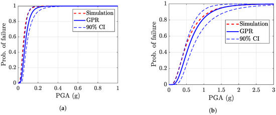
Figure 13.
Comparison of predicted fragility curves from GPR (Test Datasets 1 and 2) with those from the simulation. Shown also are the 90% confidence intervals of the GPR prediction. (a) Test Dataset 1: mm, mm. (b) Test Dataset 2: mm, mm.
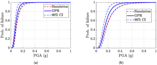
Figure 14.
Comparison of predicted fragility curves from GPR (Test Datasets 3 and 4) with those from simulation. Shown also are the 90% confidence intervals of the GPR prediction. (a) Test Dataset 3: mm, mm. (b) Test Dataset 4: mm, mm.
Coming back to Figure 12, we observed an apparent trend that simultaneously increased the column dimension and decreased the column height, leading to a higher mean and standard deviation of the lognormal distribution. Essentially, the model tells us that the structure is mainly affected by the column dimension-height ratio; this makes sense from a structural viewpoint. That is, the structure provides more resistance to earthquakes as column slenderness is decreased (assuming that the shear failure is not governing) due to a lower bending moment for a given lateral (seismic) force. The lognormal standard deviation, however, is not significantly affected by the change in b and H (see the relatively small change in the color bar of Figure 12b). The difference is affected mainly by the change in the mean of the lognormal distribution, as evidenced by the relatively large range of the values (see Figure 12a). On top of that, the slightly higher standard deviation in the smaller column dimension-height ratio is accommodated by the less sensitivity to PGA change (see Figure 7). Although the trend is apparent, making a quantitative prediction is more complicated, which is why GPR is useful, because it provides a quantitative prediction of the fragility curve.
The result essentially demonstrates that the constructed GPR models are helpful in predicting fragility curves from the simulated data, bypassing the need to perform more simulations for untested configurations. Furthermore, the result gives us a high level of confidence in extracting important insight from the GPR model. The predicted fragility curves can then be used for many purposes, e.g., predicting the fragility of an existing individual building or for design purposes. In the following sections, we show the application of GPR for predicting the population fragility curves, analyzing the impact of the input variables on the fragility curve, and assessing seismic risk.
4.2. Population Fragility Estimation
One might be interested in visualizing the family of fragility curves from a building population. In this sense, our interest was not the prediction of a single structure, but the population as defined by the given distribution. The crude use of Monte Carlo simulation is hindered by the enormous computational cost associated with a large number of simulations. The GPR model allows data-driven rapid estimation of the population fragility curve via Monte Carlo simulation applied to the surrogate models. To that end, we used the lognormal distribution’s predicted mean and standard deviation on a set of a large number of random samples. We then used the ensemble of the distributions to plot the population fragility curves. Building the population fragility curve from GPR is more computationally expensive than just a single prediction and the associated confidence interval. However, notice that such a process is still significantly less costly than a direct Monte Carlo simulation. Furthermore, plotting the minimum and maximum of the curves is not so informative. Therefore, we computed the desired percentiles (for example, the 5th and 95th percentiles) based on a large number of random fragility curves and then plotted this result. However, it is worth noting that there are uncertainties associated with the predicted fragility curves. It is then essential to provide the interval of the predicted percentiles, which can be interpreted as the uncertainty of uncertainty.
The predicted population fragility curves, in both linear and log scales, are shown in Figure 15. This figure shows the mean, the 5th, and the 95th percentile of the population fragility curves. The plot gives information on the distribution of the failure probability of all structures within the population. It can be seen that the spread is quite large, meaning that some buildings have high resistance, while others are prone to structural failure. It is interesting to see that the population fragility curves, as a whole, are not affected much by the uncertainty from the GPR model. We can then say that the estimated population fragility curves accurately represent the general trend. Although this paper assumed that b and H are uniformly distributed, notice that the method also works for any arbitrary input distribution.
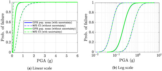
Figure 15.
Estimation of the population fragility curves from the GPR models. Shown are the population mean and the 5th and 95th percentiles with and without considering the uncertainty estimate from GPR.
4.3. Effect of Changing Parameters on Fragility Curves
Another advantage of a regression model is that it enables exploring the effect of changing the input variables on the fragility curve. The effect of changing the parameters of column height and column side length as per using the numerical simulation can be seen in Figure 7. Here, it can be seen that reducing the column height decreased the probability of collapse because of a smaller bending moment for the same lateral load level. Enlarging the column size was shown to effectively increase the column’s cross-sectional area, hence providing larger resistance (lower probability of collapse). To visualize the impact, we fixed either b or H to specific values and, then, varied the other variable. Notice that we did not include the model uncertainty to avoid a too cluttered plot. However, the trend is evident even if only the mean prediction is plotted. Figure 16 shows the result from this observation by fixing H to mm and m (i.e., the lower and upper bound of H, respectively); the column dimension was then varied from 150 to 400 mm afterwards. As shown in Figure 16a, the fragility curve was sensitive to the change in column dimension if we fixed the column height to mm. Figure 16a essentially shows that, for fixed mm, the structure’s resistance can be increased quite significantly if the column dimension is increased. On the other hand, for a fixed mm, changing the column width only slightly changed the fragility curve (pay attention to the different scaling in the PGA axis). For fixed , the structure was still largely fragile even when the column dimension was increased (see Figure 16b).
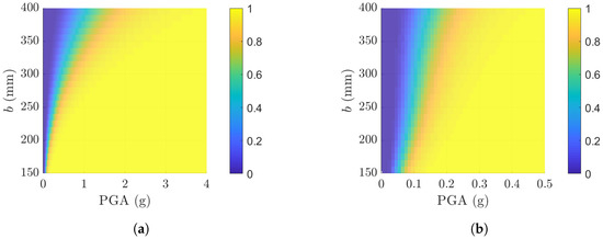
Figure 16.
Plots depicting the impact of varying the column dimension while keeping the height fixed on the fragility curve. The color bar indicates the failure probability. (a) Fixed column height at mm. (b) Fixed column height at mm.
Next, the impact of changing the column height while fixing the dimension is shown in Figure 17. Figure 17a,b depict the variation in the fragility curve by fixing the column width to mm and 400 mm, respectively. For a fixed mm case, the structure is still fragile because the variation in column height yields a non-significant effect on the fragility curve. However, the opposite is true for the fixed mm case, in which the structure is susceptible to the change in column height; decreasing the column height greatly increases the structure’s resistance. Notice that one can fix a parameter to any arbitrary value (e.g., mm) and then vary the other parameter to see the effect. Surrogate models enable such a design exploration since it is an inexpensive replacement for the original simulation.
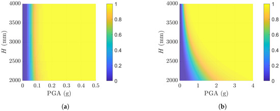
Figure 17.
Plots depicting the impact of varying the column height while keeping the dimension fixed on the fragility curve. The color bar indicates the failure probability. (a) Fixed column dimension at mm. (b) Fixed column dimension at mm.
4.4. Experiment Using Sampling Points on the Boundaries
As a side experiment, we constructed GPR models using only the boundary points of the input space. The aim was to investigate whether it is worth reducing the sample size by focusing the samples only on boundaries. The results from this investigation are shown in Figure 18. From the result, we can see that the trend of the mean of the fragility curve is predicted well. However, the prediction of the standard deviation seems erroneous, indicating the difficulty in the modeling process. Our result suggests that the sampling points should cover the design space’s interior to capture the trend accurately.
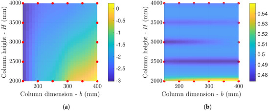
Figure 18.
Plots of GPR predictions for the mean and standard deviation of the lognormal distribution from the fragility curve using only the boundary points. (a) Mean of lognormal distribution. (b) Standard deviation of lognormal distribution.
It is also worth noting that sampling on the boundaries becomes less feasible for more than two input variables due to more points required to cover the edges. Furthermore, sampling on the boundaries is also impossible for non-uniformly distributed random inputs (e.g., Gaussian distribution) since boundaries are non-existent for such distributions. Therefore, for higher-dimensional inputs, it is recommended to use other sampling techniques such as Latin hypercube sampling or a low-discrepancy sequence to reduce the impact of the curse of dimensionality.
4.5. Seismic Risk Assessment
Besides data-driven prediction of the fragility curve, we also used GPR to directly predict the Probability of Collapse (PoC) for a given hazard in a particular region. The GPR model allows data-driven rapid computation of the PoC, which is necessary for quick assessment of a single or population of buildings. The PoC is a localized measure for a given region compared to the fragility curve. The PoC itself is a function of the fragility curve as defined in Equation (9):
In this section, we introduce two seismic hazard curves’ data to calculate the PoC, namely Bandung’s and Jakarta’s hazard curves (see Figure 19). It must be noted, however, that the fragility curves used for evaluating the risk used the results presented in the earlier section (i.e., only based on hazard deaggregation for Bandung). In practice, the fragility curves must be reanalyzed consistently based on the seismic characteristics of the investigated region. The two hazard curves were only used here to showcase how the same building population might produce different PoCs in two different regions. The calculation of the PoC can be easily performed using any numerical integration routine once the seismic hazard and fragility curve data are available.
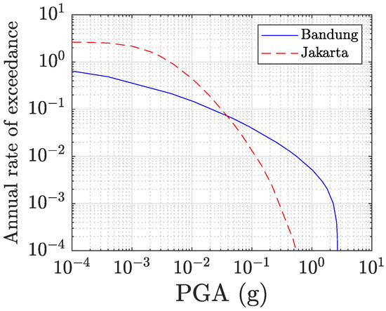
Figure 19.
Seismic hazard curve for Jakarta and Bandung.
Using the GPR model efficiently enables predicting and visualizing the collapse probability for various column dimensions and height combinations. There are two possible ways to calculate the PoC. First, we can use the GPR models of the fragility curve to predict the PoC for a given hazard. The first approach is efficient because there is no need to build further GPR models for different hazard levels; instead, we only need to post-process the fragility curve’s GPR models. Second, one can also create a GPR model directly for the PoC. This second approach requires constructing a different GPR model for a different hazard level since it corresponds to different . Nevertheless, the second approach is more straightforward because it bypasses the surrogate model’s construction in the fragility curve level, and we only need to build one model instead of two separate models (for the mean and standard deviation of the lognormal distribution). We opted for the second approach due to its straightforward nature, which also eases the computation of quantities such as uncertainty estimates. The GPR model for the one-year PoC was constructed using the PoC data from the training set. As for the 50-year PoC plot, there is no need to build a separate GPR model since it can be directly calculated from the 1-year PoC result.
Figure 20 and Figure 21 show the carpet plot of the PoC prediction for Jakarta and Bandung, respectively. For both regions, it can be clearly seen that the PoC increases as the column height increases and the column dimension decreases, which is consistent with the trend of the fragility curve shown earlier. However, the GPR model for the PoC provides a more context-dependent analysis for the given hazard level. The difference is more evident, especially for the 50-year PoC plot, due to the accumulation of risk from a 50-year trajectory. The plot also shows that the column dimension b is a more decisive factor since, for a fixed H, altering it might significantly decrease or increase the probability of collapse. Furthermore, for the 50-year plot, the GPR model predicts the boundary of where the structure conforms to the current prescribed risk stated in the Indonesian seismic codes (that is, PoC ≤ 0.01 after 50 years) on the right bottom part of the plot for Jakarta, indicating that only a small fraction of the non-engineered housing structures will likely survive the design earthquake. Alarmingly, if we consider a typical column height we found in practice (≥2500 mm), no “safe” zone is present, even with a 400 mm column size. The PoC surface plot for Bandung shows a higher risk associated with buildings in Bandung compared to Jakarta. According to the linear analysis, the 50-year PoC plot for Bandung also reveals that almost all building configurations in Bandung are highly likely to collapse after 50 years. The reason for such a higher PoC for Bandung is clear if we see Figure 19, in which high PGA values occur more frequently in Bandung than in Jakarta. In short, Bandung has a larger seismic demand than Jakarta.
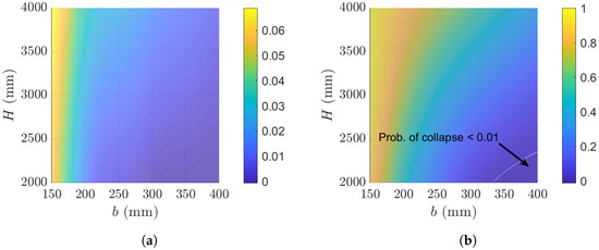
Figure 20.
GPR plots of the probability of collapse for Jakarta within the first year and after 50 years. (a) Probability of collapse (1 year). (b) Probability of collapse (50 years).
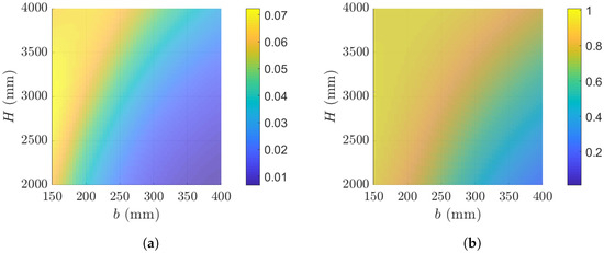
Figure 21.
GPR plots of the probability of collapse for Bandung within the first year and after 50 years. (a) Probability of collapse (1 year). (b) Probability of collapse (50 years).
In addition, Figure 22 depicts the histogram of the population’s PoC that was calculated using the Monte Carlo simulation routine applied to the GPR model. The y-axis Figure 22 was normalized to depict the probability density function. Figure 22 shows the different natures of the two regions. By observing the one-year plot for Jakarta, it can be seen that most structures are concentrated in a lower collapsing probability region (far-left region). However, the tendency to collapse is greatly magnified under the 50-year scenario, which is during the common service life of a structure, with only a few structures fulfilling the requirement that the PoC be less than 0.01 within 50 years. On the other hand, the PDF of the PoC for Bandung shows a significant shift of the curve to the right side, which means that the same building is more likely to fail in Bandung than in Jakarta. The significantly high risk of collapse for the building in Bandung is clearly evident from the corresponding 50-year PoC plot.
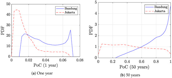
Figure 22.
Histogram of the collapsing probability as predicted by the GPR surrogate model for Bandung and Jakarta.
It is worth noting that the current estimation of the PoC was deemed conservative due to the nature of the linear elastic analysis when estimating the fragility curves. This means that we entirely neglected the potential contribution of ductility, which allows internal forces to redistribute before the building eventually reaches a collapsed state. Nevertheless, the same procedure can be applied for more realistic scenarios by simply replacing the PoC data from linear analysis with nonlinear analysis where the structure’s ductility is introduced aside from the strength resistance. Our primary goal in this study was to demonstrate the capability of GPR for aiding such tasks, regardless of the type of analysis employed.
5. Conclusions and Future Works
In this study, we demonstrated the potential use of GPR to provide a quick, yet reliable estimate of buildings’ structural capacities against earthquakes (in the form of seismic fragility curves). GPR mainly enables rapid and data-driven estimation of fragility curves for untested configurations, populations, and parameter sweep studies. In particular, GPR can be beneficial to bypass the need for individual structural analysis when a large building sample is considered. One significant advantage of GPR compared to other surrogate modeling approaches is that it provides an uncertainty estimate, which is useful for decision-making. This aspect can be essential for two practical scenarios. First, in the pre-disaster context, GPR can be used to identify the most vulnerable group of buildings that must be prioritized in a rehabilitation (strengthening) program before the next earthquake strikes. Second, in the post-disaster context, GPR can help the federal emergency agencies allocate the available resources better to help the most-affected regions first.
Two main building parameters: column height and column size, were systematically investigated in this study. Reducing the column height decreases the probability of collapse because of a smaller bending moment for the same lateral load level. Enlarging the column size has been shown to effectively increase the column’s cross-sectional area, hence providing larger resistance (lower probability of collapse). With the use of GPR, a theoretically unlimited combination of the two parameters can be analyzed in a fraction of a minute to produce the corresponding fragility curve. When more building parameters are considered, the advantages provided by GPR will be even more pronounced.
In the last section, GPR was further utilized to produce the Probability of Collapse (PoC) for a given hazard (demand). Two seismic hazard curves for Bandung and Jakarta were considered to showcase how the proposed method can be applied. The resulting PoC predictions were plotted on a contour map, showing the region deemed to fulfill the building codes’ requirements (PoC ≤ 0.01 for 50 years). Alarmingly, even for Jakarta (with a smaller hazard level than Bandung), only a small fraction of the non-engineered housing structures will likely survive the design earthquake. When comparing the PoC of housing built in Jakarta vs. Bandung, it was observed that the buildings in Bandung always have a higher PoC, which is consistent with the hazard curve. In the future, the integration of the fragility curve with spatial hazard and building information can significantly improve the understanding of the spatial risks of cities.
It must also be noted that the current calculation of the PoC was performed based on linear elastic analysis, which shall provide the lower bound of the structural resistance. However, such an assumption neglects the potential contribution of internal forces’ redistribution, which may help to enhance the resistance and delay the failure. As stated before, the primary goal of this study was to demonstrate the capability of GPR in aiding such tasks. In the future, nonlinear analysis in conjunction with practical building configurations shall be investigated to allow a more meaningful interpretation of the GPR results. From the viewpoint of surrogate models, there are several interesting research directions to pursue. First, the use of adaptive sampling can be explored since it can potentially reduce the number of simulations, which will be especially useful for handling complex, high-dimensional problems. Using GPR with advanced probabilistic modeling tools (e.g., copula) is also an interesting research direction to pursue a more realistic treatment of real-world data. Furthermore, the use of advanced GPR models such as the deep Gaussian process [53] can be explored for achieving better accuracy. Lastly, to validate the consistency of the findings from the present study, we aim to consider more record-to-record variations of ground motions for a more realistic prediction of fragility curves and see the effects on the GPR prediction in future studies. It must also be noted that the current calculation of the PoC was performed based on linear elastic analysis, which shall provide the lower bound of the structural resistance. However, such an assumption neglects the potential contribution of internal forces’ redistribution, which may help to enhance the resistance and delay the failure. As stated before, the primary goal of this study was to demonstrate the capability of GPR in aiding such tasks. In the future, nonlinear analysis in conjunction with practical building configurations shall be investigated to allow a more meaningful interpretation of the GPR results. From the viewpoint of surrogate models, there are several interesting research directions to pursue. First, the use of adaptive sampling can be explored since it can potentially reduce the number of simulations, which will be especially useful for handling complex, high-dimensional problems. Using GPR with advanced probabilistic modeling tools (e.g., copula) is also an interesting research direction to pursue a more realistic treatment of real-world data. Furthermore, the use of advanced GPR models such as the deep Gaussian process [53] can be explored for achieving better accuracy. Lastly, to validate the consistency of the findings from the present study, we aim to consider more record-to-record variations of ground motions for a more realistic prediction of fragility curves and see the effects on the GPR prediction in future studies.
Author Contributions
Conceptualization, P.W.S., P.S.P. and A.S.; methodology, P.W.S., P.S.P. and A.S.; software, P.S.P. and Y.S.; validation, Y.S.; formal analysis, P.W.S., P.S.P., Y.A. and A.S.; investigation, P.W.S., P.S.P. and Y.A.; resources, P.W.S.; data curation, P.W.S., P.S.P., Y.S., S.C.S. and I.I.; writing—original draft preparation, P.W.S., Y.A. and P.S.P.; writing—review and editing, P.W.S., P.S.P. and A.S.; visualization, P.S.P., Y.A. and A.S.; supervision, P.W.S., A.S. and I.I.; project administration, P.W.S.; funding acquisition, P.W.S. All authors have read and agreed to the published version of the manuscript.
Funding
This research was funded by Institut Teknologi Bandung through the PPMI Program.
Institutional Review Board Statement
Not applicable.
Informed Consent Statement
Not applicable.
Data Availability Statement
Data is available upon reasonable request.
Acknowledgments
We gratefully acknowledge the funding from ITB research grant under PPMI 2021 Program.
Conflicts of Interest
The authors declare no conflict of interest. The funders had no role in the design of the study; in the collection, analyses, or interpretation of data; in the writing of the manuscript; or in the decision to publish the results.
References
- WHO. World Health Statistics 2018: Monitoring Health for the SDGs, Sustainable Development Goals; World Health Organization: Geneva, Switzerland, 2018. [Google Scholar]
- Struyk, R.J.; Hoffman, M.L.; Katsura, H.M. The Market for Shelter in Indonesian Cities; The Urban Insitute: Washington, DC, USA, 1990. [Google Scholar]
- Arya, A.S.; Boen, T.; Ishiyama, Y. Guidelines for Earthquake Resistant Non-Engineered Construction; UNESCO: Paris, France, 2014. [Google Scholar]
- Watanabe, S.; Shima, N.; Fujita, K. Research on non-engineered housing construction based on a field investigation in Jakarta. J. Asian Archit. Build. Eng. 2013, 12, 33–40. [Google Scholar] [CrossRef]
- Narafu, T.; Sugiyama, H.; Imai, H.; Tasaka, A.; Nakajima, Y. Basic Study on Earthquake Safety Masonry Constructions in Developing Countries-comparative experiments of cement mortar. AIJ J. Technol. Des. 2009, 15, 637–642. [Google Scholar] [CrossRef]
- Griffith, M.C.; Ingham, J.M.; Weller, R. Earthquake reconnaissance: Forensic engineering on an urban scale. Aust. J. Struct. Eng. 2010, 11, 63–74. [Google Scholar] [CrossRef]
- Cogurcu, M. Construction and design defects in the residential buildings and observed earthquake damage types in Turkey. Nat. Hazards Earth Syst. Sci. 2015, 15, 931–945. [Google Scholar] [CrossRef]
- Lizundia, B.; Durphy, S.; Griffin, M.; Holmes, W.; Hortacsu, A.; Kehoe, B.; Porter, K.; Welliver, B. Update of FEMA P-154: Rapid visual screening for potential seismic hazards. In Improving the Seismic Performance of Existing Buildings and Other Structures 2015; FEMA: Washington, DC, USA, 2015; pp. 775–786. [Google Scholar]
- Benedetti, D.; Petrini, V. On seismic vulnerability of masonry buildings: Proposal of an evaluation procedure. L’Industria Delle Costr. 1984, 18, 66–74. [Google Scholar]
- Grant, D.N.; Bommer, J.J.; Pinho, R.; Calvi, G.M.; Goretti, A.; Meroni, F. A prioritization scheme for seismic intervention in school buildings in Italy. Earthq. Spectra 2007, 23, 291–314. [Google Scholar] [CrossRef]
- Grünthal, G. European Macroseismic Scale 1998; Technical Report; European Seismological Commission (ESC): Luxemburg, 1998. [Google Scholar]
- Sobester, A.; Forrester, A.; Keane, A. Engineering Design via Surrogate Modelling: A Practical Guide; John Wiley & Sons: New York, NY, USA, 2008. [Google Scholar]
- Bhosekar, A.; Ierapetritou, M. Advances in surrogate based modeling, feasibility analysis, and optimization: A review. Comput. Chem. Eng. 2018, 108, 250–267. [Google Scholar] [CrossRef]
- Yan, Y.; Huang, H.; Sun, L. Multivariate structural seismic fragility analysis and comparative study based on moment estimation surrogate model and Gaussian copula function. Eng. Struct. 2022, 262, 114324. [Google Scholar] [CrossRef]
- Esteghamati, M.Z.; Flint, M.M. Developing data-driven surrogate models for holistic performance-based assessment of mid-rise RC frame buildings at early design. Eng. Struct. 2021, 245, 112971. [Google Scholar] [CrossRef]
- Anwar, G.A.; Dong, Y. Surrogate-based decision-making of community building portfolios under uncertain consequences and risk attitudes. Eng. Struct. 2022, 268, 114749. [Google Scholar] [CrossRef]
- Rasmussen, C.E. Gaussian processes in machine learning. In Proceedings of the Summer School on Machine Learning; Springer: New York, NY, USA, 2003; pp. 63–71. [Google Scholar]
- Gentile, R.; Galasso, C. Gaussian process regression for seismic fragility assessment of building portfolios. Struct. Saf. 2020, 87, 101980. [Google Scholar] [CrossRef]
- Guo, M.; Hesthaven, J.S. Reduced order modeling for nonlinear structural analysis using Gaussian process regression. Comput. Methods Appl. Mech. Eng. 2018, 341, 807–826. [Google Scholar] [CrossRef]
- Echard, B.; Gayton, N.; Lemaire, M. AK-MCS: An active learning reliability method combining Kriging and Monte Carlo simulation. Struct. Saf. 2011, 33, 145–154. [Google Scholar] [CrossRef]
- Liu, Z.; Lu, Z.; Ling, C.; Feng, K.; Hu, Y. An improved AK-MCS for reliability analysis by an efficient and simple reduction strategy of candidate sample pool. Structures 2022, 35, 373–387. [Google Scholar] [CrossRef]
- Dutta, S. A sequential metamodel-based method for structural optimization under uncertainty. Structures 2020, 26, 54–65. [Google Scholar] [CrossRef]
- Wang, X.; Zhang, J.; Sun, Y.; Wu, Z.; Tchuente, N.F.C.; Yang, F. Stiffness identification of deteriorated PC bridges by a FEMU method based on the LM-assisted PSO-Kriging model. Structures 2022, 43, 374–387. [Google Scholar] [CrossRef]
- Ereiz, S.; Duvnjak, I.; Jiménez-Alonso, J.F. Review of finite element model updating methods for structural applications. Structures 2022, 41, 684–723. [Google Scholar] [CrossRef]
- Moustapha, M.; Bourinet, J.M.; Guillaume, B.; Sudret, B. Comparative study of Kriging and support vector regression for structural engineering applications. ASCE-ASME J. Risk Uncertain. Eng. Syst. Part A Civ. Eng. 2018, 4, 04018005. [Google Scholar] [CrossRef]
- Nieto, F.; Montoya, M.C.; Hernández, S.; Kusano, I.; Casteleiro, A.; Alvarez, A.J.; Jurado, J.Á.; Fontán, A. Aerodynamic and aeroelastic responses of short gap twin-box decks: Box geometry and gap distance dependent surrogate based design. J. Wind. Eng. Ind. Aerodyn. 2020, 201, 104147. [Google Scholar] [CrossRef]
- Bernardini, E.; Spence, S.M.; Wei, D.; Kareem, A. Aerodynamic shape optimization of civil structures: A CFD-enabled Kriging-based approach. J. Wind. Eng. Ind. Aerodyn. 2015, 144, 154–164. [Google Scholar] [CrossRef]
- Sarli, P.; Sanjaya, Y.; Azhari, Y.; Setiawan, A. On The Behaviour of Non-Engineered Residential Buildings in Bandung, Indonesia: A Study Case. In Proceedings of the 17th World Conference on Earthquake Engineering, Sendai, Japan, 13–18 September 2020; International Association of Earthquake Engineering: Sendai, Japan, 2021. [Google Scholar]
- Kusumastuti, D.; Suarjana, M.; Pribadi, K.; Rildova; Lie, T. Experimental Study on Typical Confined Masonry Structure under Cyclic Lateral Load. In Proceedings of the 15th World Conference on Earthquake Engineering, Lisbon, Portugal, 24–28 September 2012; International Association of Earthquake Engineering: Lisbon, Portugal, 2012. [Google Scholar]
- ASCE/SEI 41-17; Seismic Evaluation and Retrofit of Existing Buildings. American Society of Civil Engineers: New York, NY, USA, 2017.
- Pusat Studi Gempa Nasional. Peta Sumber dan Bahaya Gempa Indonesia Tahun 2017; Kementrian Pekerjaan Umum dan Perumahan Rakyat: Bandung, Indonesia, 2017. (In Indonesian) [Google Scholar]
- Asrurifak, M.; Irsyam, M.; Hutapea, B.; Mahesworo, R.; Ridwan, M.; Aldiamar, F. Peta Deagregasi Hazard Gempa Indonesia Untuk Periode Ulang Gempa 2475 Tahun. In Annual Indonesian Geotechnical Engineering Conference; Himpunan Ahli Tanah Indonesia: Jakarta, Indonesia, 2017. (In Indonesian) [Google Scholar]
- Sari, A.; Soebowo, E.; Syahbana, A.; Tohari, A. Microzonation of Soil Amplification Based on Microtremor, Spt and Cptu Data in Bandung Basin. Ris. Geol. Dan Pertamb. 2019, 29, 53. [Google Scholar] [CrossRef]
- Cao, X.Y.; Feng, D.C.; Wang, Z.; Wu, G. Parametric investigation of the assembled bolt-connected buckling-restrained brace and performance evaluation of its application into structural retrofit. J. Build. Eng. 2022, 48, 103988. [Google Scholar] [CrossRef]
- Baker, J.W. Efficient analytical fragility function fitting using dynamic structural analysis. Earthq. Spectra 2015, 31, 579–599. [Google Scholar] [CrossRef]
- Vamvatsikos, D.; Cornell, C.A. Incremental dynamic analysis. Earthq. Eng. Struct. Dyn. 2002, 31, 491–514. [Google Scholar] [CrossRef]
- Council, A.T. Quantification of Building Seismic Performance Factors; U.S. Department of Homeland Security; FEMA: Washington, DC, USA, 2009.
- Jalayer, F. Direct Probabilistic Seismic Analysis: Implementing Non-Linear Dynamic Assessments; Stanford University: Stanford, CA, USA, 2003. [Google Scholar]
- Pang, Y.; Wang, X. Cloud-IDA-MSA conversion of fragility curves for efficient and high-fidelity resilience assessment. J. Struct. Eng. 2021, 147, 04021049. [Google Scholar] [CrossRef]
- Straub, D.; Der Kiureghian, A. Improved seismic fragility modeling from empirical data. Struct. Saf. 2008, 30, 320–336. [Google Scholar] [CrossRef]
- O’Reilly, G.J. Limitations of Sa (T1) as an intensity measure when assessing non-ductile infilled RC frame structures. Bull. Earthq. Eng. 2021, 19, 2389–2417. [Google Scholar] [CrossRef]
- Zelaschi, C.; Monteiro, R.; Pinho, R. Improved fragility functions for RC bridge populations. In Proceedings of the 5th ECCOMAS Thematic Conference on Computational Methods in Structural Dynamics and Earthquake Engineering, Island, Greece, 25–27 May 2015; pp. 25–27. [Google Scholar]
- Suzuki, A.; Iervolino, I. Intensity measure conversion of fragility curves. Earthq. Eng. Struct. Dyn. 2020, 49, 607–629. [Google Scholar] [CrossRef]
- Nguyen, D.D.; Thusa, B.; Azad, M.S.; Tran, V.L.; Lee, T.H. Optimal earthquake intensity measures for probabilistic seismic demand models of ARP1400 reactor containment building. Nucl. Eng. Technol. 2021, 53, 4179–4188. [Google Scholar] [CrossRef]
- Katsanos, E.I.; Sextos, A.G.; Manolis, G.D. Selection of earthquake ground motion records: A state-of-the-art review from a structural engineering perspective. Soil Dyn. Earthq. Eng. 2010, 30, 157–169. [Google Scholar] [CrossRef]
- Shome, N.; Cornell, C.A.; Bazzurro, P.; Carballo, J.E. Earthquakes, records, and nonlinear responses. Earthq. Spectra 1998, 14, 469–500. [Google Scholar] [CrossRef]
- Giovenale, P.; Cornell, C.A.; Esteva, L. Comparing the adequacy of alternative ground motion intensity measures for the estimation of structural responses. Earthq. Eng. Struct. Dyn. 2004, 33, 951–979. [Google Scholar] [CrossRef]
- Kohrangi, M.; Vamvatsikos, D.; Bazzurro, P. Implications of intensity measure selection for seismic loss assessment of 3-D buildings. Earthq. Spectra 2016, 32, 2167–2189. [Google Scholar] [CrossRef]
- Grigoriu, M. Do seismic intensity measures (IMs) measure up? Probabilistic Eng. Mech. 2016, 46, 80–93. [Google Scholar] [CrossRef]
- Luco, N.; Ellingwood, B.R.; Hamburger, R.O.; Hooper, J.D.; Kimball, J.K.; Kircher, C.A. Risk-Targeted versus Current Seismic Design Maps for the Conterminous United States. U.S. Geological Survey. 2007. Available online: http://pubs.er.usgs.gov/publication/70045059 (accessed on 13 December 2022).
- Yakut, A.; Yılmaz, H. Correlation of deformation demands with ground motion intensity. J. Struct. Eng. 2008, 134, 1818–1828. [Google Scholar] [CrossRef]
- Hansen, N.; Ostermeier, A. Completely derandomized self-adaptation in evolution strategies. Evol. Comput. 2001, 9, 159–195. [Google Scholar] [CrossRef] [PubMed]
- Damianou, A.; Lawrence, N.D. Deep Gaussian processes. In Proceedings of the 16th International Conference on Artificial Intelligence and Statistics, Scottsdale, AZ, USA, 29 April–1 May 2013; Volume 31, pp. 207–215. [Google Scholar]


Disclaimer/Publisher’s Note: The statements, opinions and data contained in all publications are solely those of the individual author(s) and contributor(s) and not of MDPI and/or the editor(s). MDPI and/or the editor(s) disclaim responsibility for any injury to people or property resulting from any ideas, methods, instructions or products referred to in the content. |
© 2022 by the authors. Licensee MDPI, Basel, Switzerland. This article is an open access article distributed under the terms and conditions of the Creative Commons Attribution (CC BY) license (https://creativecommons.org/licenses/by/4.0/).