Abstract
Understanding the deterioration mechanism of concrete structures in cold climates that are susceptible to frost damage from repeated freezing and thawing cycles is imperative for ensuring their durability and serviceability. This study analyzed the impact of freeze–thaw (FT) exposure on concrete structural behavior by developing three machine-learning approaches—artificial neural networks (ANN), random forests (RF), and support vector machines (SVM)—to quantify the progressive loss in compressive strength after repeated FT cycles. The results demonstrate that all of the proposed models can predict the deteriorated compressive strength of concrete and align closely with the experimental results. The ANN model demonstrated the highest prediction accuracy with an R2 of 0.924, exhibiting a higher prediction accuracy than RF and SVM models. Sensitivity analysis using Shapley additive explanations (SHAP) revealed that concrete with an initially high strength, along with a lower water–cement ratio and air entrainment, exhibited the least reduction in compressive strength after freezing–thawing cycles, underlining the positive impact of these factors on the FT durability of concrete. The proposed modeling approach accurately predicts the residual compressive strength after FT exposure, enabling the selection of optimal concrete materials and structural designs for cold climates.
1. Introduction
In cold regions, concrete structures undergo repeated freeze–thaw cycles (FTCs) as temperatures fluctuate around freezing. During FTCs, water trapped within concrete’s pores freezes and expands, creating internal hydraulic pressures that can damage the concrete’s structure [1,2]. Upon thawing, more water can penetrate the damaged concrete and lead to cumulative deterioration over successive FTCs. This progressive freeze–thaw damage can significantly degrade concrete’s load-bearing performance, durability, and structural safety over time [3,4,5,6]. Consequently, assessing the load-bearing capability of these deteriorating concrete structures is becoming increasingly important. Previously, various standard testing procedures, including the ASTM C666 [7], GB/T 50083-2009 [8], JIS A1148:2010 [9], and RILEM CIF test [10], were applied to experimentally determine the frost resistance of concrete by measuring different properties of concrete before and after FTCs as specified by these standards, such as the relative dynamic elastic modulus (RDEM), mass loss, strength loss, and length change. Based on ASTM C666, Shi [11] examined cylindrical concrete specimens subjected to FTCs and found that the mechanical properties of the specimens had significantly decreased. Shang and Song [12] evaluated the uniaxial and biaxial behavior of frost-damaged concrete using the GB/T 50083-2009 FTC test standard, similar to ASTM C666, and reported notable reductions in strength and durability. Duan et al. [13] conducted experiments on confined and unconfined prismatic concrete samples according to GB/T 50083-2009 and proposed the degradation models, using FTC numbers as the damage index. Diao et al. [14] examined the combined effect of FTCs, steel corrosion, and sustained load on the structural behavior of reinforced concrete beams. They identified accelerated degradation and more rapid strength loss when FTCs, corrosive exposure, and sustained loads occurred simultaneously. Petersen et al. [15] applied RILEM standard and studied the influence of FTCs on the elastic modulus and interface bond behavior of concrete. Their results demonstrated a reduced modulus and bond strength in concrete specimens damaged by freeze–thaw exposure. These experimental studies collectively emphasize the detrimental impact of FTCs on concrete structures, highlighting reductions in mechanical properties, increased vulnerability to cracking, and structural degradation. While these experiments provide crucial insights, they often vary in terms of specimen sizes, test parameters, and environmental conditions, leading to dispersed results and uncertainties.
In addition to the experiments, a number of studies have been undertaken to theoretically verify the damage evaluation of concrete materials. For example, a certain amount of literature explores the connections among various damage indices (i.e., strength, stiffness, ultrasonic wave velocity), and more stable relationships can be observed [16,17,18]. Other researchers introduced these damage indices by utilizing plastic tensile strain, which is induced by freezing expansion, and mesoscale analyses have been undertaken to demonstrate this concept [19,20,21,22]. Although empirical models to estimate the mechanical deterioration of concrete were proposed, their applicability was restricted to specific test conditions, and they could not be applied universally [16,17,23,24,25]. While prior studies have explored the deterioration of concrete from FTCs through empirical modeling, there remain several knowledge gaps. Most existing empirical models are limited in their ability to universally predict strength deterioration under diverse FT conditions due to differences in specimen characteristics, test parameters, and techniques. Furthermore, the majority of research has focused on relating damage indices through experiments, with a limited emphasis on developing comprehensive mathematical models incorporating both materials and environmental variables.
Recently, machine-learning (ML) techniques have gained popularity and have been utilized to explore the complex behavior of a number of civil engineering structures [26,27,28]. Several researchers have attempted to assess the varied performances of concrete using ML techniques. Zhang et al. [29] predicted 28-day strength using industrial data for 12,107 concrete mixes, finding ML models outperformed previous laboratory-based models. Li et al. [30] provided a comprehensive review on ML applications in concrete science, discussing implementation, strengths, limitations, and future directions. Young et al. [31] analyzed a large field dataset of over 10,000 strength measurements, comparing predictive performance across statistical and ML techniques. Zhang et al. [32] developed ML models to classify observations of slumps of field concrete into characteristic ranges based on industrial mix data, finding that gradient boosting and RF performed best for multi-class slump prediction. Liu et al. [33] predicted the frost resistance of recycled aggregate concrete using ANN, multivariate adaptive regression spline, and Gaussian process regression based on the durability factor value. Wu et al. [34] estimated the frost durability of high-performance concrete in terms of RDEM by utilizing the recursive feature-elimination-based RF model. Zhang et al. [35] predicted the 7-day compressive strength for a dataset of field concrete mixes using nine different machine-learning models. Their work identified RF as the top performing algorithm and assessed the relative importance of mix ingredients on early strength development. These works demonstrate ML algorithms’ capabilities for uncovering complex data relationships and delivering accurate predictions for diverse concretes across ingredients, mixing methods, curing conditions, and measured properties. However, existing studies have mainly utilized ML techniques to estimate concrete mechanical performance, while research on concrete durability based on material and environmental variables is limited.
This study aims to address these gaps by leveraging ML techniques to develop generalized models for estimating the deteriorated compressive strength (DCS) of frost-damaged concrete based on an extensive compiled dataset of prior experiments, which can cover material and experimental test discrepancies. The developed models can be applied universally to predict FT durability across diverse materials and conditions. This research provides new insights into the key parameters influencing frost deterioration and enables a more reliable assessment of infrastructure safety in cold climates. For this purpose, the ANN, RF, and SVM approaches were chosen, and an overview of these computational methods is provided. Afterwards, FT-resistance prediction models were developed using a dataset compiled from the literature. The predictive performance of the models was evaluated and compared using statistical metrics such as the R-squared (R2), mean absolute error (MAE), and root mean squared error (RMSE). Additionally, a sensitivity analysis was conducted to quantify the relative importance of each input variable in driving the model predictions of frost resistance.
2. Machine-Learning (ML) Techniques Overview
Modeling deterioration in concrete structures from repetitive FTCs is complex, with material ingredients and environmental conditions influencing the nonlinear progressive damage. To address this complex modeling challenge, three advanced machine-learning techniques, ANN, SVM, and RF, were employed. These algorithms were selected given their demonstrated capabilities in capturing complex nonlinear phenomena, flexibility in modeling diverse types of data relationships, and proven effectiveness in related civil engineering applications. An overview of how these techniques function is provided in the following sections.
2.1. Artificial Neural Network (ANN)
ANN is a data-handling-related computing algorithm that addresses highly nonlinear regression and classification issues and can investigate complicated correlations in high-dimensional data [36,37]. A well-trained ANN model can deliver reliable findings while requiring less processing than conventional numerical analysis [38]. ANNs are made of layered structures including several nodes arranged in a pattern. These layers can be categorized as input, hidden, and output layers. The artificial neuron receives input data, which can provide an output when processed by a mathematical function. The setup of an ANN comprises the following essential steps: (1) establishing the ANNs architecture; (2) defining the necessary training algorithm for the ANN’s learning phase; and (3) determining the mathematical functions representing the mathematical model. The architecture of the ANN determines how the artificial neurons are organized inside the network and how data are transmitted between nodes. The network is referred to as a multilayer ANN when neurons are placed in several layers. The training phase optimizes an ANN model by minimizing an error function that quantifies the difference between the model’s predictions and the true training data outputs. Training employs techniques like gradient descent to iteratively adjust the inter-node weights and biases to reduce this error across many iterations. As training progresses, the model becomes increasingly refined at mapping inputs to outputs as evidenced by a decreasing error. When the model achieves a low enough error threshold, this indicates the completion of training. The optimized model with final weighted connections can accurately generalize to new data.
2.2. Random Forest (RF)
RF is a regression and classification ensemble created by Leo Breiman at the University of California, Berkeley [39]. The RF model is derived from the classification and regression tree (CART) approach to generate more precise output predictions. It builds many decision trees to forecast the outcome, with the growth of each tree being determined by a random collection of predictors [40]. Bagging is the approach used to combine all of the created decision trees into one, and it is applied to an RF model to reduce the related prediction variance. The random samples of training data must be taken for every decision tree; this is known as a bootstrap sample. The selected approach produces predictions by applying the decision tree algorithm to the chosen bootstrap samples. The final output value in the RF model is the mean of the output values obtained from all decision trees. Therefore, the final value of prediction can be derived as follows [41]:
where shows the output value for the i tree.
2.3. Support Vector Machine (SVM)
SVM is a well-known statistical ML model designed by Vapnik [42]. It is efficient in enhancing generalization performance and capable of obtaining globally optimum and unique solutions. SVM has demonstrated an excellent performance in both regression and classification applications; hence, it has been widely used. When SVM is used in regression analysis, it is frequently referred to as support vector regression (SVR). The fundamental goal of SVR is to reduce the maximum allowed generalization error according to structural risk minimization (SRM) [43]. In nonlinear scenarios, kernel functions selected beforehand in the SVM method enable data transfer from a lower-dimensional space to a higher-dimensional space to locate a linearly independent hyperplane. Table 1 lists the most commonly used kernel functions [44], where γ, d, xi, and xj, indicate the kernel function coefficient, dimension of the input vector, training pattern, and test pattern, respectively.

Table 1.
Different types of SVM kernel functions.
3. Research Methodology
3.1. Variable Selection
It is well known that the deterioration of concrete’s performance due to frost damage is a complicated process [45,46,47,48]. Several experiments have been performed in accordance with the above standards to look at how the properties of frost-damaged concrete change over time. However, it is hard to find a model that can be used for all of the laboratory experiments, even when the standards are not followed exactly. In order to make a good prediction model that can account for differences in materials and experimental tests, this paper collected 155 sets of test data as a database [49,50,51,52] and utilized ML models to predict the strength reduction in concrete under frost attack. The input variables used in this study are the number of FTCs, initial compressive strength (CS), water–cement ratio (W/C), maximum temperature during each FT cycle (Max T), minimum temperature during each FT cycle (Min T), and air-entrainment (AE). The output variable is the DCS under frost attack. For the air-entrainment type, ‘0’ and ‘1’ represent non-air-entrained and air-entrained frost-damaged concrete, respectively (see Appendix A).
3.2. Data Characterization
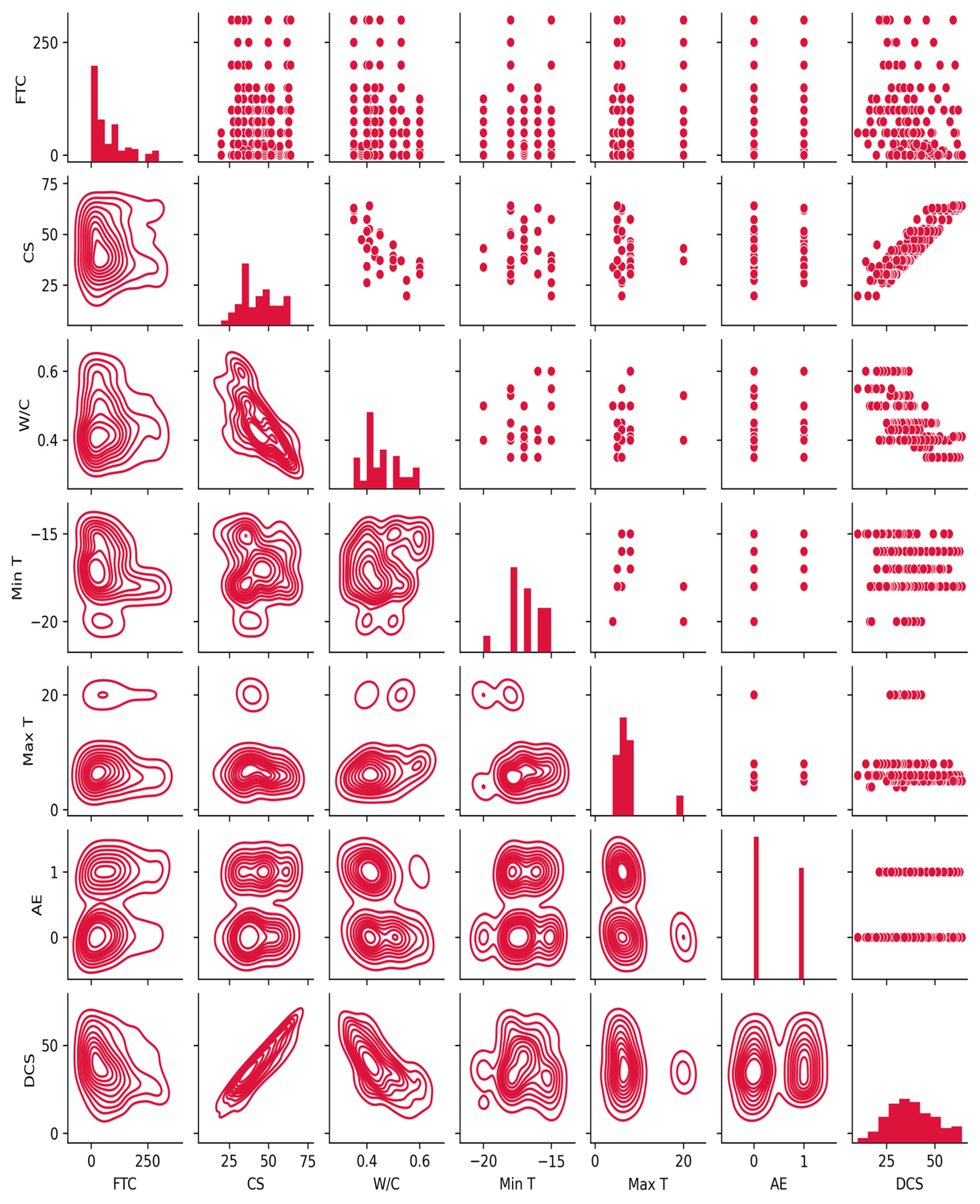
Figure 1 provides a preliminary analysis of the distribution characteristics for the 8 input variables by generating a scatter matrix plot. The diagonal shows the histogram frequency distributions for each variable, providing insight into the shape and skew. The lower left scatter plots visualize the joint probability density, with darker colors indicating a higher density of observations. The upper right scatter plots showcase the bivariate relationships between the different variables, providing insights into the specific distributions of the data. The nonlinear relationships observed among multiple input variables suggest that linear regression or simple nonlinear models may not accurately capture the data distributions and their effects on the output variables. More sophisticated nonlinear modeling techniques are likely needed to analyze these multivariate relationships. Table 2 provides descriptive statistics summarizing the distributional characteristics of the 7 variables used in this study.
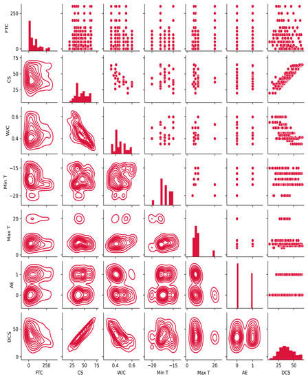
Figure 1.
Distribution of data characteristics of input and output variables.

Table 2.
Exploratory analysis of variables.
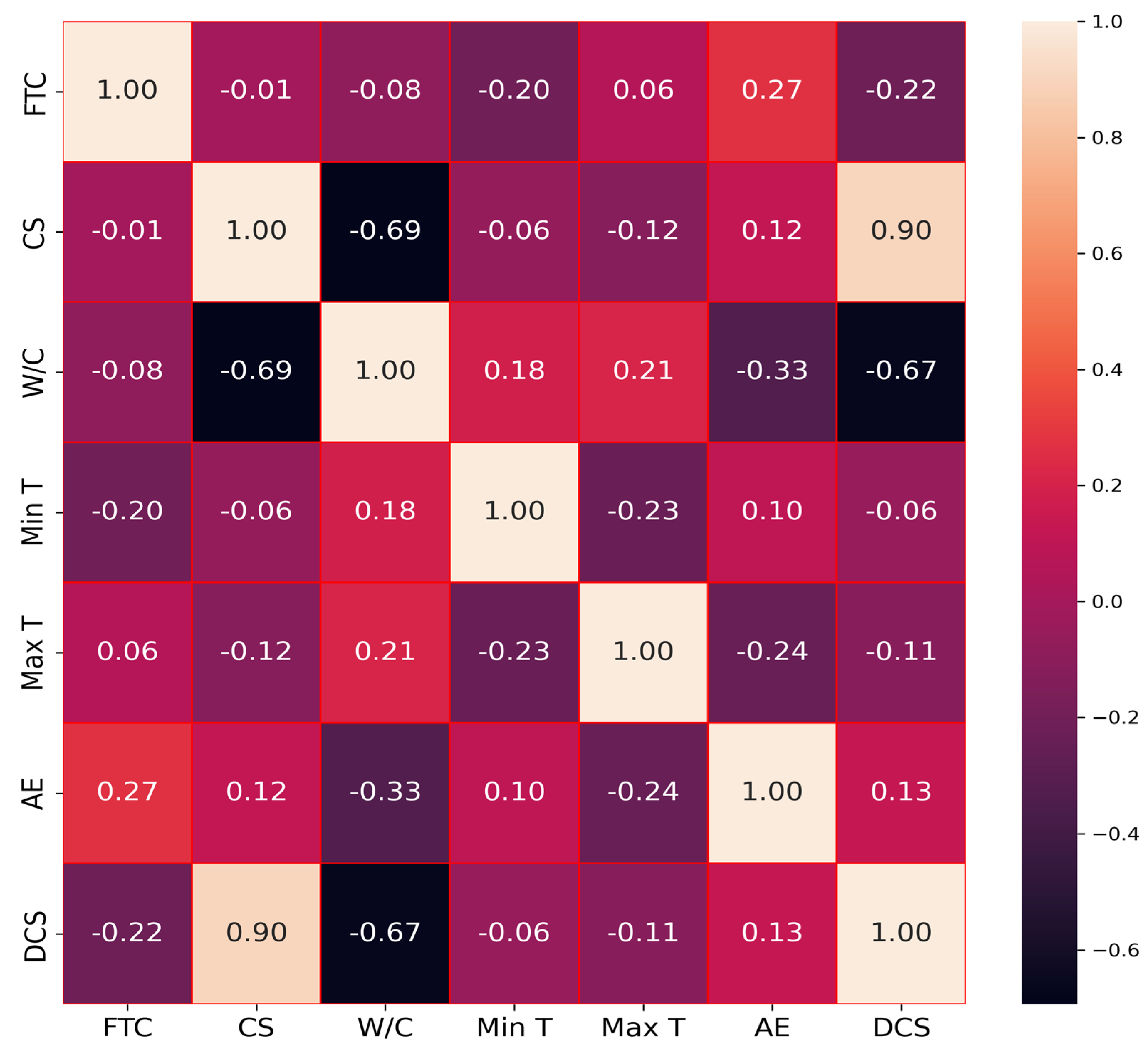
The Pearson correlation coefficient, which assesses the link between inputs and outputs, is a significant and frequently used indicator in the design of ML models. Therefore, this coefficient was developed to examine the inter-dependency and multi-collinearity between six input variables and one output parameter. The Pearson correlation coefficient has a range of −1 to 1. The values close to 0 represent weaker correlations, while values close to −1 and 1 indicate stronger negative and positive correlations, respectively. As shown in Figure 2, moderate to strong correlations exist between the input variables FTC, CS, W/C ratio, Max T, Min T, and AE and the output variable DCS, suggesting these variables have good predictive relationships.

Figure 2.
Pearson correlation coefficient matrix.
3.3. Data Preprocessing
In the present study, the min–max normalization approach was used to normalize the six input parameters and the one output parameter. The purpose of this technique is to normalize all the data between 0 and 1 to enhance the model’s performance, as unscaled variables in regression problems may result in explosive gradients, hence failing the learning process [53]. This normalization was calculated using Python’s min–max scaler preprocessing function from the Scikitlearn module. The acquired data were divided into training and testing datasets; 80% of the data were used to train models, while the remaining 20% were used to evaluate the accuracy of the trained models.
3.4. Model Performance Evaluation
It is important to assess model performance while training statistical and data-driven models so that hyperparameter tuning can be repeated until the ideal model is chosen [54]. There are a variety of well-established metrics for measuring predictive performance. These metrics, in conjunction with model diagnostic plots and the visualization of anticipated and actual values, provide a complete view of model performance.
Three evaluation metrics were employed to assess the effectiveness of the presented models: the mean absolute error (MAE), the root mean squared error (RMSE), and the coefficient of determination (R2) which can be defined as follows:
where represent the total number of observations, experimental, and anticipated response values, respectively. are the average of the experimental and anticipated response values, respectively. A model with excellent predictions gives lower MAE and RMSE values and a greater R2 value.
3.5. Proposed Model
Three distinct ML models, such as ANN, SVM, and RF, were utilized to estimate the DCS of frost-damaged concrete, considering the combined effect of multiple factors. A 5-fold cross-validation was utilized as a robust technique to select and validate the performance of our machine-learning models. It served a crucial role in optimizing the hyperparameters of these models, ensuring their generalization capability to unseen data in the testing phase. Error metrics were computed for each fold of the training and testing dataset. Furthermore, each model’s mean metrics were compared to establish the most accurate model for predicting DCS. In addition, a sensitivity analysis was conducted using Shapley additive explanations (SHAP) to assess the impact of different input features on the model output. SHAP is a technique that calculates the contribution of each input variable to an individual model prediction. It does this by comparing what the model predicts with and without a variable, weighting the comparisons based on all possible combinations [55,56]. The SHAP values indicate how much each variable influences the prediction either positively or negatively. This provides interpretable insights into the relative importance of variables. The following diagram in Figure 3 summarizes these procedures. This research uses the open-source Python modules Matplotlib, Numpy, Pandas, and Scikitlearn to create ML models.
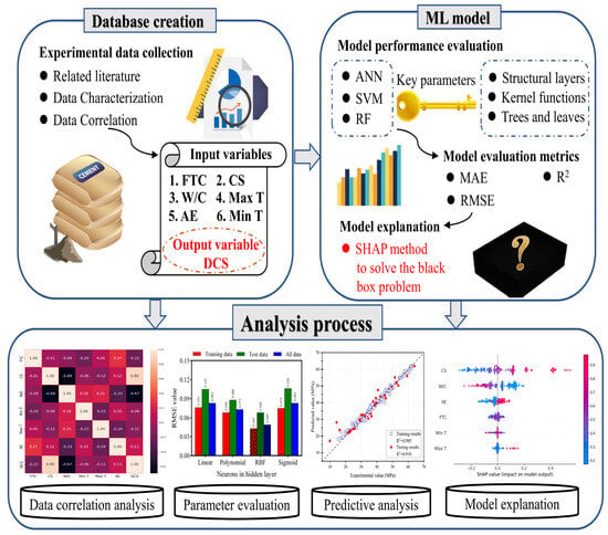
Figure 3.
Proposed organizational scheme to predict DCS.
4. Results and Discussions
4.1. Model Development
4.1.1. ANN Model
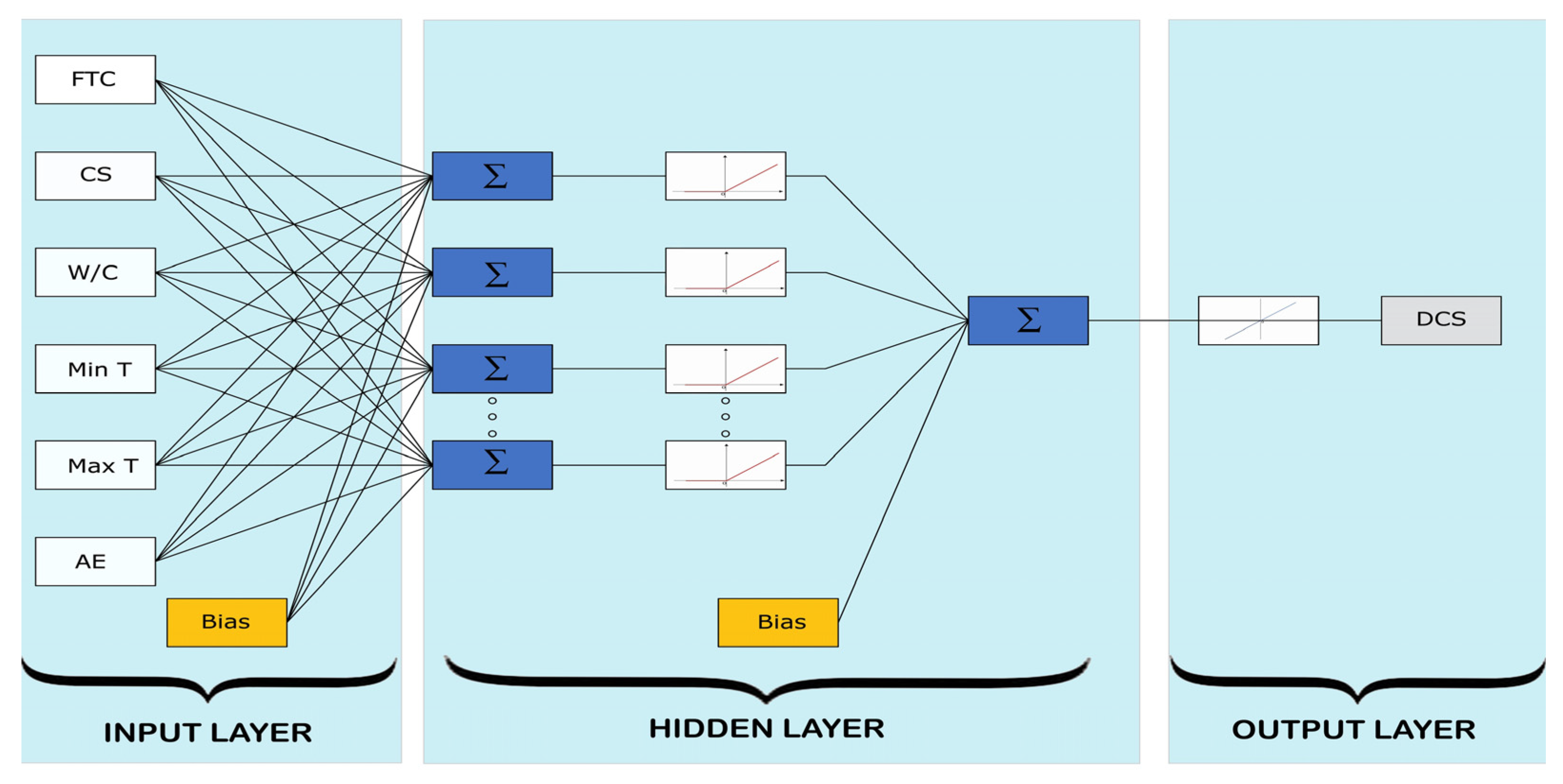
In general, an ANN model’s architecture significantly impacts its efficiency, but there is no standard method of comparison. Consequently, trial and error methods are frequently utilized. In the present study, a three-layered feedforward network with a back propagation algorithm was employed. One hidden layer consisting of 5 to 15 neurons was considered as shown in Figure 4. The rectified linear unit function and the identity transfer function were applied for the activation functions of the hidden and output layers, respectively. Due to the random selection of initial weights and biases, 10 iterations of each model were conducted to discover the ideal one.
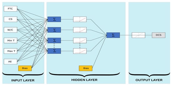
Figure 4.
Architecture of ANN models.
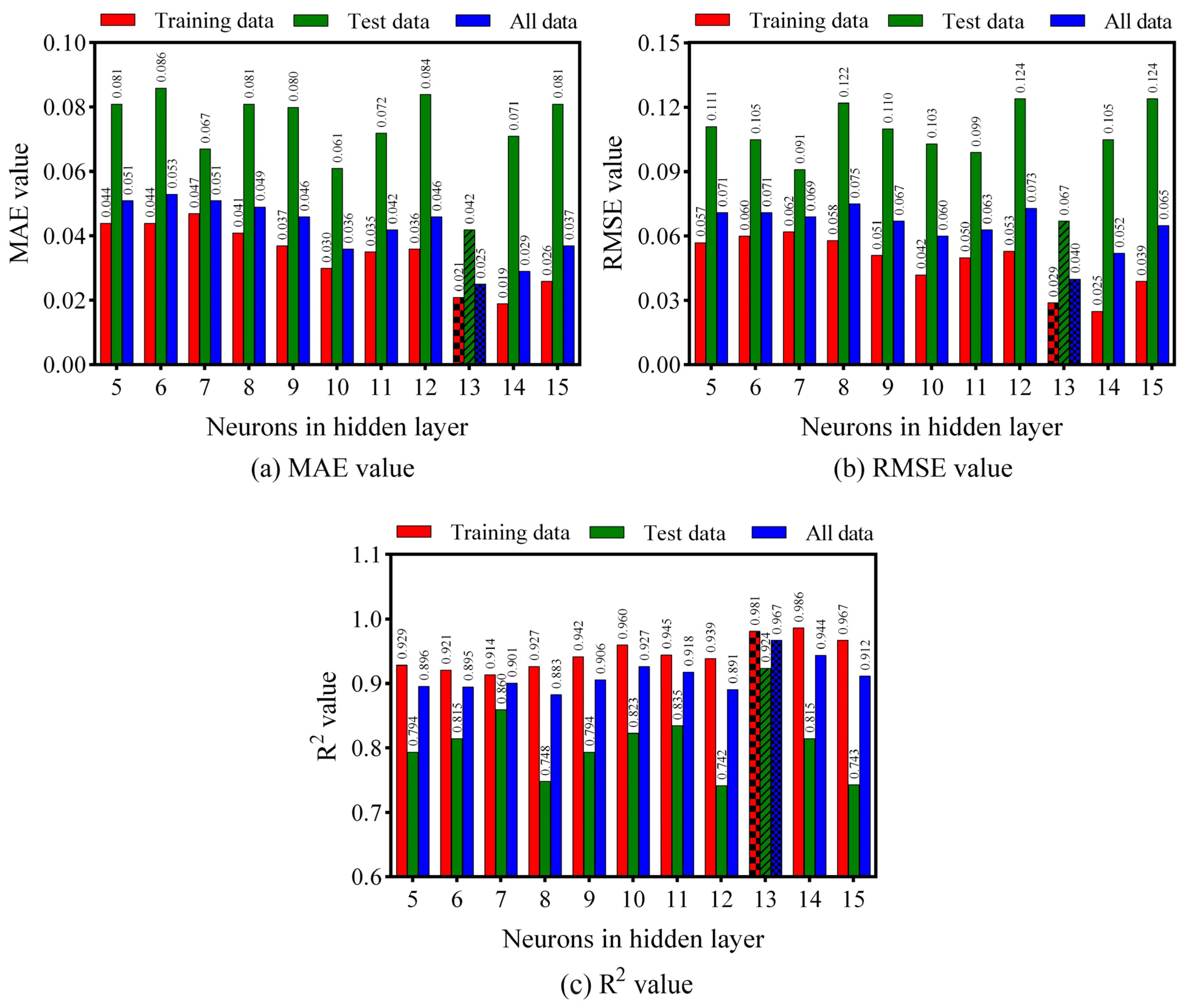
Different ANN model architectures were compared in terms of their performance, as shown in Figure 5. It can be seen that the ANN model with 13 neurons in the hidden layer exhibits an excellent efficiency with the lowest MAE (0.021 for the training data, 0.0420 for the testing data, and 0.025 for all data) and RMSE (0.029 for the training data, 0.067 for the testing data, and 0.04 for all data), and the highest R2 (0.981 for the training data, 0.924 for the testing data, and 0.967 for all data).

Figure 5.
ANN model performance with different architectures.
4.1.2. RF Model
The RF architecture is strongly affected by the number of grown trees and the maximum depth of tree. It is known from random forest theory that as the number of grown trees rises, the random forest model will progressively converge and stabilize unless the number of grown trees is excessively large. It will result in a slower convergence rate for the model, which is undesirable for practical applications [57]. Choosing an adequate number of grown trees and the maximum depth of tree is therefore vital when developing an RF model.
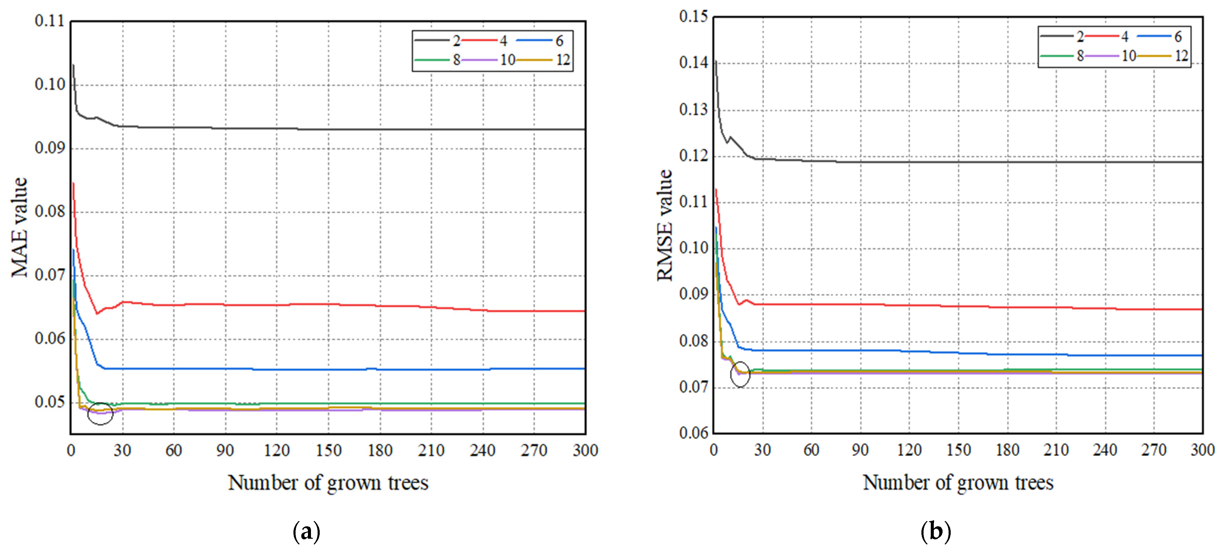
In this study, the number of grown trees varied from 1 to 300, and six different maximum depth of tree values were introduced as 2, 4, 6, 8, 10, and 12. The MAE and RMSE were used as performance indicators to find the ideal number of grown trees and leaf size. Figure 6 depicts the change trend graphs of MAE and RMSE to calculate the optimal number of grown trees and the maximum tree depth. The horizontal and vertical axes represent the number of grown trees and error values, respectively. Based on the detailed analysis, the optimal RF model design consists of 15 grown trees with a maximum depth of tree equal to 10.
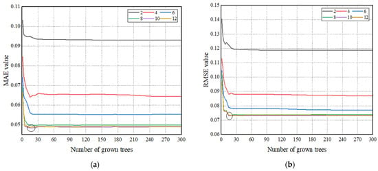
Figure 6.
Performance metrics values in function of decision trees and leaf size number. (a) MAE value. (b) RMSE value.
4.1.3. SVM Model
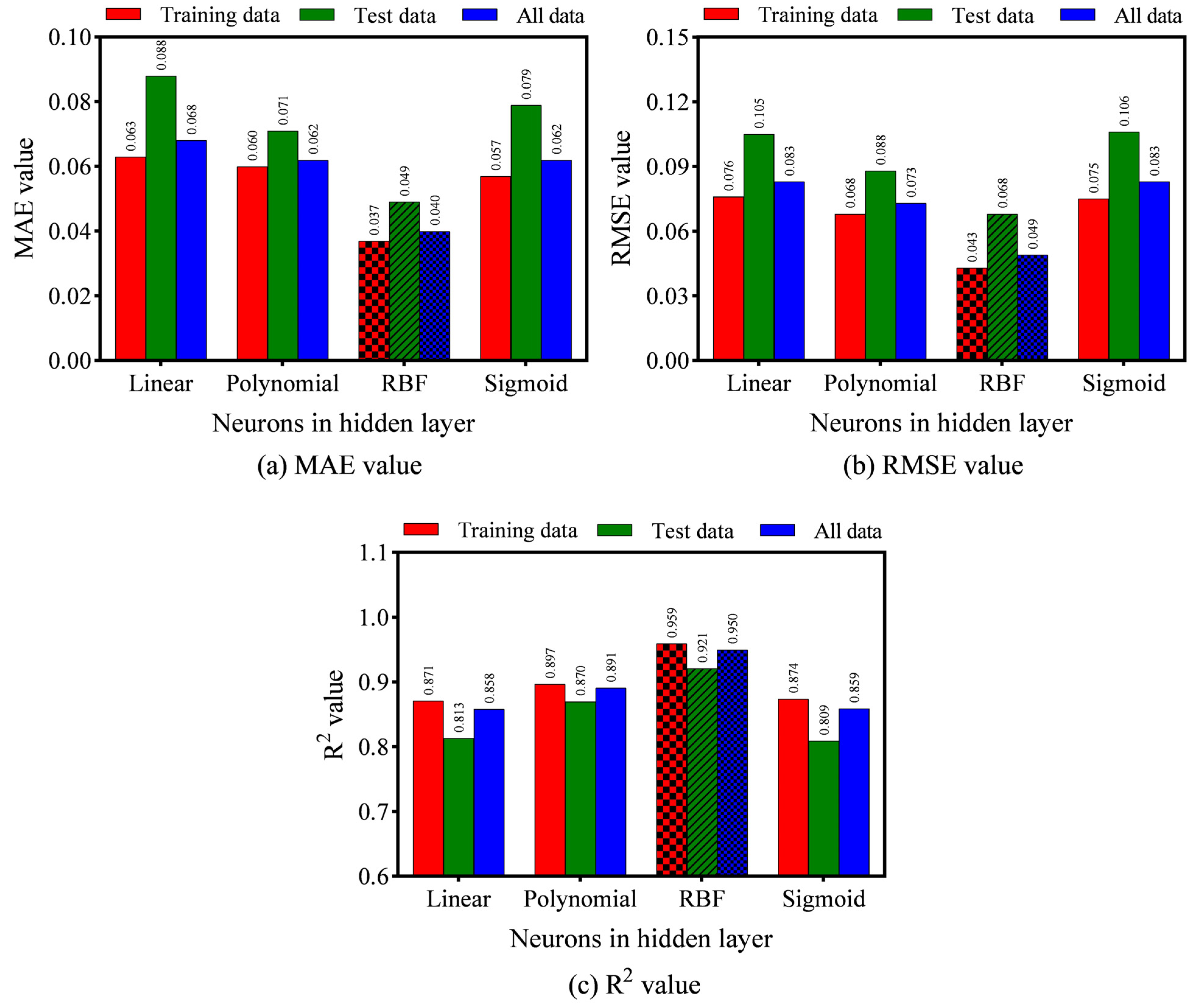
Choosing a model that gives the optimum generalization for a specific data set is essential, as several model parameters, including C, ε, γ, and d, apply to the SVM kernel functions. Therefore, the values of model parameters must be provided to forecast the target variable (i.e., DCS) based on the input variables using SVM. Choosing the appropriate model parameters for a specific kernel function considerably impacts the SVM model’s accuracy and precision. However, there is no proper method to determine those parameters. The best model parameter values were determined in this study using the trial and error technique. For this purpose, various combinations of model parameters were tested to obtain the optimum performance. Table 3 displays the appropriate modelling parameters for different kernels to estimate DCS. Error metrics were compared to determine the most appropriate kernel to use, as shown in Figure 7. According to the detailed analysis of the RMSE, MAE, and R2 values, the SVM model with the RBF kernel displayed the highest level of performance. The model reached the optimal penalty parameter C = 7.16, and that of the radial basis kernel parameter was γ = 0.18945. A smaller value of C would result in under-fitting, whereas a larger value of C would result in over-fitting; therefore, both cases might hinder the SVM model’s generalization.

Table 3.
SVM kernels model parameters’ values.

Figure 7.
Performance of SVM models with different kernel functions.
4.2. Comparison Results for ML Techniques
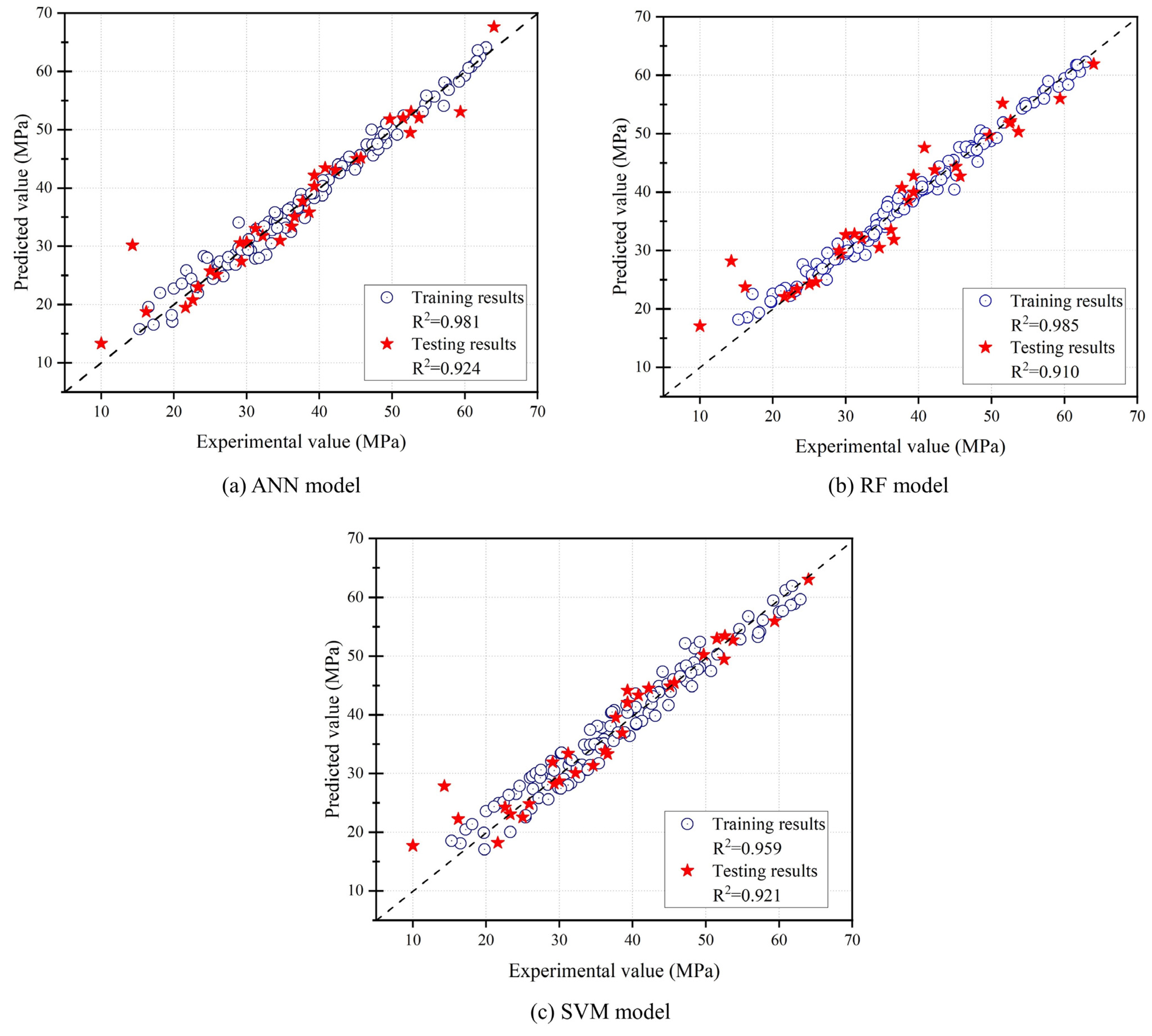
A comparison of the constructed ANN, RF, and SVM models using statistical indices, as illustrated in Table 4, is provided in this section. During the training process, the RF model’s performance surpassed the other models, with the smallest values for RMSE and MAE and the highest value for R2. The ANN model predicted the testing data well, with R2 values equaling 0.924, followed by the SVM model. The SVM model demonstrated superior stability and generalization capabilities with the minimum difference between the training and testing R2 values. The R2 score for the training and testing datasets for the RF model decreased from 0.985 to 0.910, indicating considerable overfitting. The ANN model’s overall performance was superior to that of the SVM and RF models.

Table 4.
Developed models’ statistical performance.
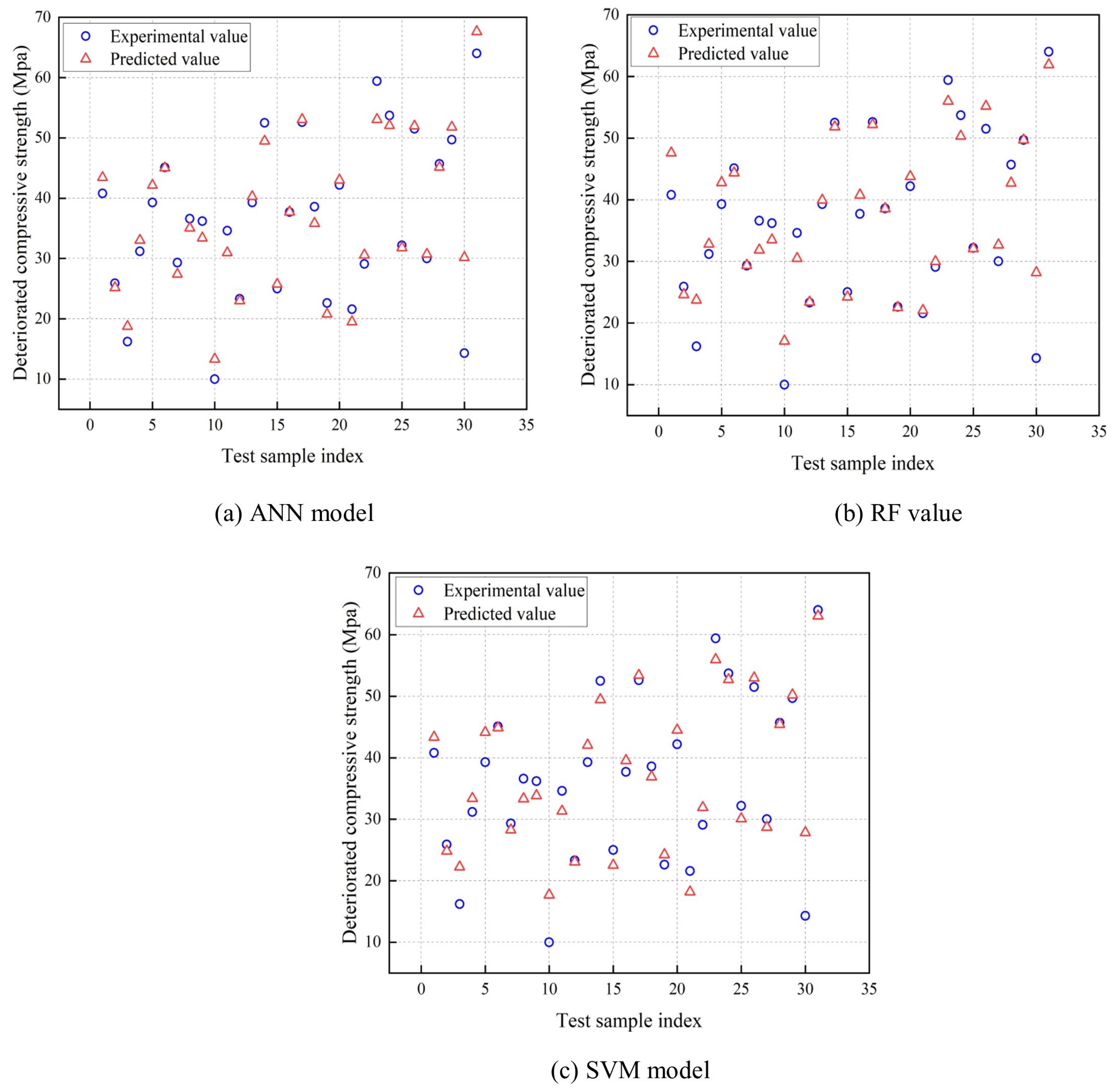
Using the training dataset to generate the models, the testing dataset was then used to evaluate the generalization capability of each model. The DCS values measured in the experimental test data were validated with the predicted values by the various ML models in Figure 8. In the testing dataset, the experimental values for CS ranged from 10 to 64 MPa. All of the models were able to fully understand the nonlinear relationship between the features of the dataset in order to predict the DCS with a similar trend between the predicted and experimental output.
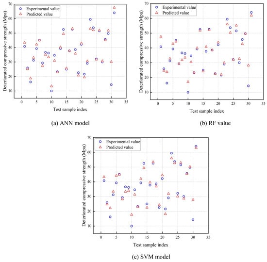
Figure 8.
Validation of experimental and predicted DCS.
The scatterplot was utilized to visualize the connection between the experimental and predicted values. A good correlation and prediction show data more closely aligned with the scatterplot’s regression line [58,59]. Figure 9 compares the experimental and predicted values of the proposed ML models for the test and training datasets. The data points with distributions closest to the regression line are included in the ANN model. When examining the scatter plots of other models, there are considerably more deviations from the regression line. Due to the small dataset available for the models, a high R2 value for the training data (up to 0.98 for the ANN and RF models) was attained. To prevent model overfitting during testing, the hyper-parameters of the models were adjusted during training to minimize the difference between the R2 values for the testing and training data.
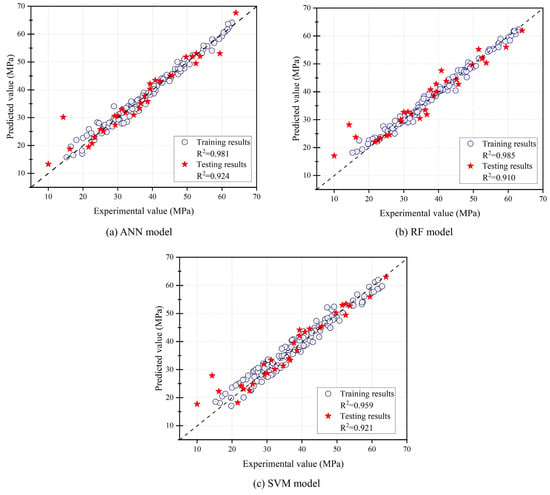
Figure 9.
Comparison of the experimental and predicted values obtained by machine learning.
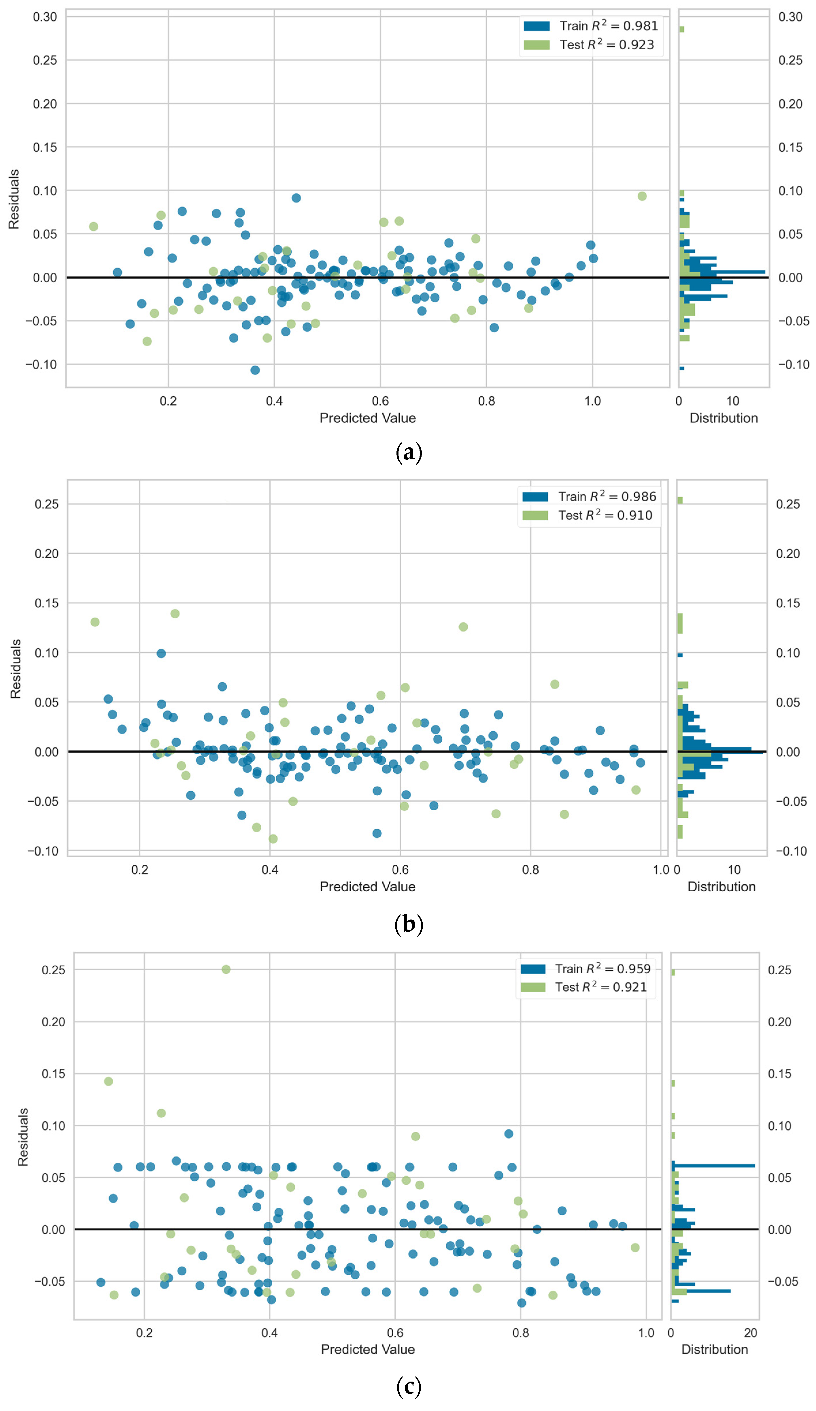
The accuracy and predictive capabilities of machine-learning models can also be compared using the residual plots, as shown in Figure 10. In this plot, the x-axis shows normalized predicted values, while the y-axis shows residuals, which demonstrate the differences between the actual and predicted values. Analyzing the residual plot for all of the proposed machine-learning models reveals a favorable outcome, characterized by a random and uniformly distributed placement of residuals around zero. There are no observable patterns or trends, indicating that our models have successfully captured underlying data relationships. However, a closer look reveals that the ANN model has a slightly higher accuracy than the SVM and RF models. This is evidenced by the ANN model’s more concentrated and centered residual distribution. When compared to the other models, these findings indicate that the ANN model has a slight edge in efficiently capturing the underlying data relationships.
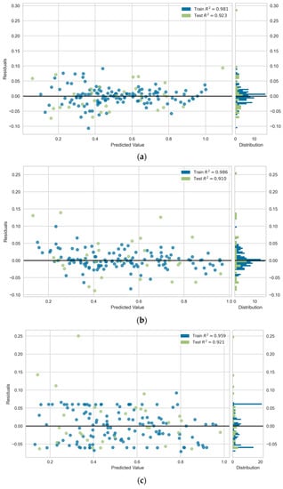
Figure 10.
Residual plots of the proposed models. (a) ANN model. (b) RF model. (c) SVM model.
4.3. Sensitivity Analysis
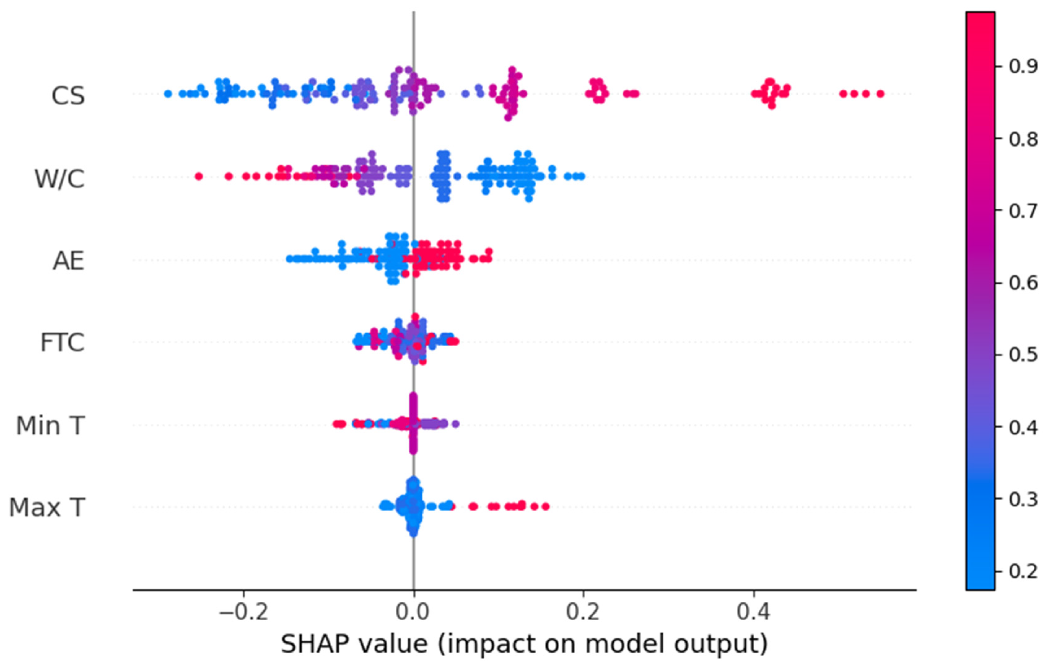
In this study, the Shapley additive explanations (SHAP) approach, which defines how an ML model gives individual predictions, was used to assess the impact of input parameters on the DCS for the ANN model. For each prediction, SHAP calculates how much each model’s input variable has contributed to the output [60,61]. The relation of different features with the DCS of concrete under frost attack is represented by SHAP values (Figure 11). The vertical axis represents the variable’s name in ascending order of significance. The number to the right of their names is the mean SHAP value. The position of a point along the horizontal axis offers information regarding the effect of a specific feature on the model’s output. Each point in the plot represents a unique instance of the database. The relative value of each attribute is shown by the color bar on the right. For instance, the initial compressive strength of concrete has a maximum SHAP value for the DCS estimate. This demonstrates that concrete with a higher initial compressive strength experiences less strength loss when subjected to frost damage than concrete with a lower initial compressive strength, since a higher initial strength of concrete is often correlated with superior durability due to the high compactness in the structure. Likewise, AE also has a positive impact on the FT durability of concrete. Figure 11 depicts the second-highest SHAP value for the W/C ratio. However, it has a detrimental effect, which means that the compressive strength declined further as the W/C ratio increased. Similarly, FTCs also negatively affect the concrete’s ability to resist freezing. Other attributes such as Min T and Max T have slight but distinct effects on the DCS.
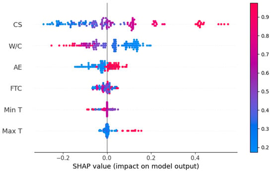
Figure 11.
SHAP summary plot for the ANN model.
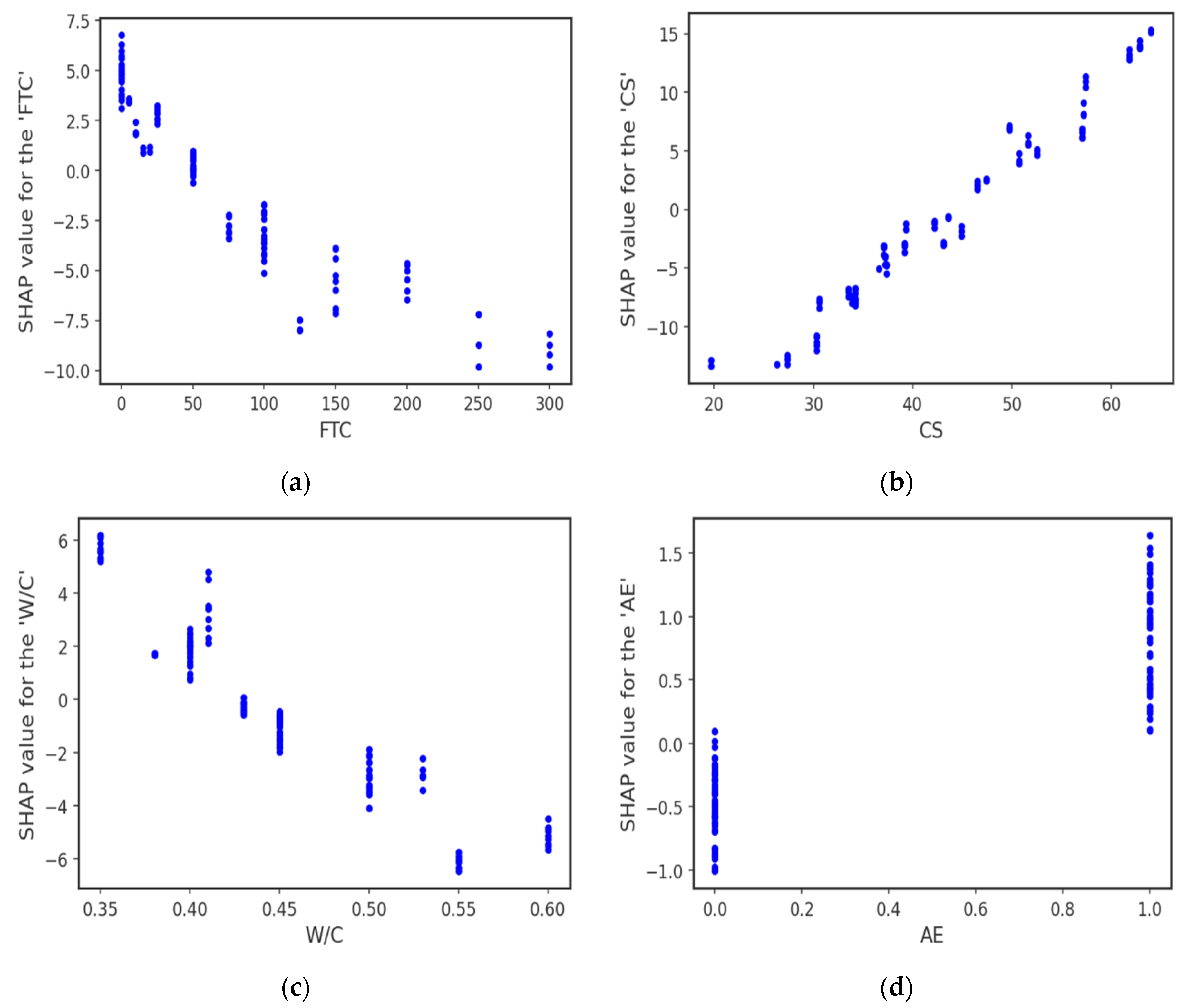
The interaction of different input features with the DCS of concrete under frost attack is depicted in Figure 12. The FTC feature interaction is shown in Figure 12a, illustrating FTC’s negative impact on DCS. Increasing the number of FTCs leads to degradation in concrete strength, resulting in a decreasing trend. Figure 12b illustrates that CS significantly positively impacts the DCS of concrete, and the SHAP values increase as CS increases. The W/C feature interaction is provided in Figure 12c which displays a negative impact of W/C on DCS. Furthermore, AE has a positive effect on DCS because the tiny air spaces created by AE serve as empty chambers for the freezing and migrating water to enter. This allows the pressure in the pores to decrease and stops the concrete from becoming damaged.
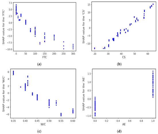
Figure 12.
SHAP input features interaction plot. (a) FTC. (b) CS. (c) W/C. (d) AE.
5. Conclusions and Recommendations
The use of ML methods to predict concrete’s mechanical properties has become more prevalent in the construction industry recently. The primary objective of this study was to assess the accuracy of ML algorithms for estimating the DCS of frost-damaged concrete and to investigate the influence of environmental factors on frost resistance that have not been previously investigated. In conclusion, this research represents an important step in the field of performance evaluation of concrete structures, particularly in cold and wet climates. By employing ML techniques, specifically ANN, RF, and SVM, we effectively constructed a model of concrete frost resistance based on the DCS due to FTCs. The study emphasizes the practical importance of using ML algorithms to estimate frost resistance because this provides accurate predictions and is more cost-effective than traditional laboratory methods. The key findings are as follows:
- (1)
- The ANN model with 13 neurons in the hidden layer exhibits the best performance, as evaluated by the lowest values for RMSE and MAE and the highest value for R2.
- (2)
- The optimal number of decision trees for the RF model is 15, and the optimal maximum depth of the tree is 10, with the MAE, RMSE, and R2 values for testing datasets being 0.048, 0.072, and 0.910, respectively.
- (3)
- The SVM model with the RBF kernel function delivers the most accurate results compared to other kernel functions (linear, polynomial, and sigmoid) based on a detailed evaluation of the MAE, RMSE, and R2 values.
- (4)
- The developed ANN model has the greatest performance among all ML models for estimating the DCS, with the MAE, RMSE, and R2 values for testing datasets being 0.042, 0.067, and 0.924, respectively, followed by the SVM and RF models. The ANN and SVM models exhibit strong stability and generalization abilities; however, the RF model overfits during training.
- (5)
- The CS of concrete has the highest influence on the DCS of concrete under frost attack, followed by the W/C ratio, AE, and the number of FTCs, as revealed through SHAP observations. The feature interaction plot illustrates that CS positively influences the DCS of concrete under frost attack while FTCs affect it negatively.
The research presented in this article has significant real-world implications for the construction industry, particularly in cold climate regions prone to FT cycles. By leveraging ML algorithms including ANN, RF, and SVM, the study provides a robust and accurate method to estimate the deteriorated compressive strength of concrete structures. This predictive capability can be applied in real time to evaluate the structural health and safety of existing concrete infrastructure in cold areas. In addition, the implementation of ML techniques can eliminate the need for labor-intensive and costly laboratory tests, making freeze-resistance assessments more accessible and feasible in engineering projects around the world. Furthermore, understanding the effects of environmental factors such as the number of FT cycles, water–cement ratio, and minimum temperature on frost resistance allows engineers and architects to make more informed decisions when designing durable, long-lasting concrete structures. As a result, this study provides engineers with valuable insights, paving the way for more efficient and trustworthy methods of assessing the frost resistance of concrete. Ultimately, this research contributes to the sustainable growth and environmental resilience of concrete structures.
While the study has already demonstrated the effectiveness of methods like ANN, RF, and SVM, there is potential for improvement. Advanced techniques such as XGBoost and CatBoost could be investigated for their potential to enhance prediction accuracy. Additionally, future research should consider incorporating additional evaluation measures such as the variance accounted for (VAF), RMSE observations standard deviation ratio (RSR), and weighted mean absolute percentage error (WMAPE) to provide a more comprehensive assessment of the model performance. These measures can contribute to a deeper understanding of the accuracy and reliability of models in predicting concrete frost resistance.
Author Contributions
Funding acquisition, F.G.; investigation, M.A.u.h.; methodology, M.A.u.h.; project administration, F.G.; software, M.A.u.h. and F.G.; supervision, W.X. and M.A.; visualization, M.A.u.h.; writing—original draft, M.A.u.h. and F.G.; writing—review and editing, W.X., M.A. and F.G. All authors have read and agreed to the published version of the manuscript.
Funding
This work was sponsored by the National Key Research and Development Program of China (No. 2022YFC3801800), Open Research Fund Program of the State Key Laboratory of Hydroscience and Engineering (sklhse-2023-C-05), and the National Natural Science Foundation of China (51820105012). The authors extend their gratitude to all of the people who participated in this work.
Informed Consent Statement
Not applicable.
Data Availability Statement
The data presented in this study are available on request from the corresponding author after obtaining permission from the authorized person.
Conflicts of Interest
The authors declare no conflict of interest.
Appendix A

Table A1.
Experimental dataset of frost-damaged concrete.
Table A1.
Experimental dataset of frost-damaged concrete.
| Source | Standard | FTC (No.) | CS (MPa) | W/C | Min T (℃) | Max T (°C) | AE (0/1) | DCS (MPa) |
|---|---|---|---|---|---|---|---|---|
| Shang et al. [12] | GB/T 50082-2009 | 0 | 34.2 | 0.5 | −15 | 6 | 0 | 34.2 |
| 25 | 34.2 | 0.5 | −15 | 6 | 0 | 30 | ||
| 50 | 34.2 | 0.5 | −15 | 6 | 0 | 24.1 | ||
| 75 | 34.2 | 0.5 | −15 | 6 | 0 | 21.7 | ||
| Cao et al. [24] | GB/T 50082-2009 | 0 | 39.2 | 0.43 | −17 | 8 | 0 | 39.2 |
| 25 | 39.2 | 0.43 | −17 | 8 | 0 | 37 | ||
| 50 | 39.2 | 0.43 | −17 | 8 | 0 | 34.7 | ||
| 75 | 39.2 | 0.43 | −17 | 8 | 0 | 31.5 | ||
| 100 | 39.2 | 0.43 | −17 | 8 | 0 | 29.3 | ||
| 125 | 39.2 | 0.43 | −17 | 8 | 0 | 26 | ||
| 0 | 46.5 | 0.41 | −17 | 8 | 1 | 46.5 | ||
| 25 | 46.5 | 0.41 | −17 | 8 | 1 | 45.1 | ||
| 50 | 46.5 | 0.41 | −17 | 8 | 1 | 42.8 | ||
| 75 | 46.5 | 0.41 | −17 | 8 | 1 | 40.4 | ||
| 100 | 46.5 | 0.41 | −17 | 8 | 1 | 37.7 | ||
| 125 | 46.5 | 0.41 | −17 | 8 | 1 | 35.8 | ||
| Fan et al. [62] | GB/T 50082-2009 | 0 | 33.9 | 0.5 | −20 | 4 | 0 | 33.9 |
| 25 | 33.9 | 0.5 | −20 | 4 | 0 | 33.9 | ||
| 50 | 33.9 | 0.5 | −20 | 4 | 0 | 30.2 | ||
| 100 | 33.9 | 0.5 | −20 | 4 | 0 | 16.2 | ||
| 125 | 33.9 | 0.5 | −20 | 4 | 0 | 17.2 | ||
| Guan et al. [63] | GB/T 50082-2009 | 0 | 37.1 | 0.53 | −18 | 20 | 0 | 37.1 |
| 50 | 37.1 | 0.53 | −18 | 20 | 0 | 35.4 | ||
| 100 | 37.1 | 0.53 | −18 | 20 | 0 | 32.4 | ||
| 150 | 37.1 | 0.53 | −18 | 20 | 0 | 31.6 | ||
| 200 | 37.1 | 0.53 | −18 | 20 | 0 | 29.9 | ||
| 250 | 37.1 | 0.53 | −18 | 20 | 0 | 29.3 | ||
| 300 | 37.1 | 0.53 | −18 | 20 | 0 | 26.8 | ||
| Hao et al. [64] | GB/T 50082-2009 | 0 | 39.3 | 0.5 | −15 | 8 | 0 | 39.3 |
| 25 | 39.3 | 0.5 | −15 | 8 | 0 | 38.6 | ||
| 50 | 39.3 | 0.5 | −15 | 8 | 0 | 36.2 | ||
| 75 | 39.3 | 0.5 | −15 | 8 | 0 | 34.6 | ||
| 100 | 39.3 | 0.5 | −15 | 8 | 0 | 32.7 | ||
| Ma et al. [65] | ASTM C666-97 | 0 | 57.2 | 0.4 | −17 | 8 | 0 | 57.2 |
| 50 | 57.2 | 0.4 | −17 | 8 | 0 | 48.7 | ||
| 100 | 57.2 | 0.4 | −17 | 8 | 0 | 40.4 | ||
| 0 | 44.9 | 0.5 | −17 | 8 | 0 | 44.9 | ||
| 50 | 44.9 | 0.5 | −17 | 8 | 0 | 32 | ||
| 100 | 44.9 | 0.5 | −17 | 8 | 0 | 20 | ||
| 0 | 43.6 | 0.4 | −17 | 8 | 1 | 43.6 | ||
| 50 | 43.6 | 0.4 | −17 | 8 | 1 | 40.9 | ||
| 100 | 43.6 | 0.4 | −17 | 8 | 1 | 38 | ||
| 0 | 37.4 | 0.5 | −17 | 8 | 1 | 37.4 | ||
| 50 | 37.4 | 0.5 | −17 | 8 | 1 | 31.3 | ||
| 100 | 37.4 | 0.5 | −17 | 8 | 1 | 24.6 | ||
| Zhang et al. [66] | GB/T 50082-2009 | 0 | 57.4 | 0.4 | −15 | 8 | 0 | 57.4 |
| 10 | 57.4 | 0.4 | −15 | 8 | 0 | 54.7 | ||
| 50 | 57.4 | 0.4 | −15 | 8 | 0 | 49.2 | ||
| 100 | 57.4 | 0.4 | −15 | 8 | 0 | 40.8 | ||
| 0 | 36.6 | 0.6 | −15 | 8 | 0 | 36.6 | ||
| 10 | 36.6 | 0.6 | −15 | 8 | 0 | 28.9 | ||
| 50 | 36.6 | 0.6 | −15 | 8 | 0 | 14.3 | ||
| 0 | 33.5 | 0.6 | −15 | 8 | 1 | 33.5 | ||
| 10 | 33.5 | 0.6 | −15 | 8 | 1 | 32.2 | ||
| 50 | 33.5 | 0.6 | −15 | 8 | 1 | 31.2 | ||
| 100 | 33.5 | 0.6 | −15 | 8 | 1 | 23.1 | ||
| Shang et al. [67] | GB/T 50082-2009 | 0 | 26.3 | 0.4 | −15 | 6 | 1 | 26.3 |
| 100 | 26.3 | 0.4 | −15 | 6 | 1 | 25.9 | ||
| 200 | 26.3 | 0.4 | −15 | 6 | 1 | 23.3 | ||
| 300 | 26.3 | 0.4 | −15 | 6 | 1 | 22.6 | ||
| Shang et al. [68] | GB/T 50082-2009 | 0 | 50.7 | 0.45 | −18 | 6 | 0 | 50.7 |
| 25 | 50.7 | 0.45 | −18 | 6 | 0 | 45.2 | ||
| 50 | 50.7 | 0.45 | −18 | 6 | 0 | 37.5 | ||
| 75 | 50.7 | 0.45 | −18 | 6 | 0 | 35.2 | ||
| 0 | 27.4 | 0.55 | −18 | 6 | 0 | 27.4 | ||
| 25 | 27.4 | 0.55 | −18 | 6 | 0 | 22.4 | ||
| 50 | 27.4 | 0.55 | −18 | 6 | 0 | 18.1 | ||
| 75 | 27.4 | 0.55 | −18 | 6 | 0 | 16.5 | ||
| 0 | 34.2 | 0.4 | −18 | 6 | 1 | 34.2 | ||
| 50 | 34.2 | 0.4 | −18 | 6 | 1 | 33.4 | ||
| 100 | 34.2 | 0.4 | −18 | 6 | 1 | 31.7 | ||
| 150 | 34.2 | 0.4 | −18 | 6 | 1 | 27.6 | ||
| 200 | 34.2 | 0.4 | −18 | 6 | 1 | 26.4 | ||
| 300 | 34.2 | 0.4 | −18 | 6 | 1 | 21.1 | ||
| Xiao et al. [69] | GB/T 50082-2009 | 0 | 61.8 | 0.35 | −18 | 6 | 1 | 61.8 |
| 50 | 61.8 | 0.35 | −18 | 6 | 1 | 60.9 | ||
| 100 | 61.8 | 0.35 | −18 | 6 | 1 | 59.2 | ||
| 150 | 61.8 | 0.35 | −18 | 6 | 1 | 55.8 | ||
| 200 | 61.8 | 0.35 | −18 | 6 | 1 | 52.6 | ||
| 250 | 61.8 | 0.35 | −18 | 6 | 1 | 49.3 | ||
| 300 | 61.8 | 0.35 | −18 | 6 | 1 | 45.6 | ||
| 0 | 49.7 | 0.45 | −18 | 6 | 1 | 49.7 | ||
| 50 | 49.7 | 0.45 | −18 | 6 | 1 | 48.9 | ||
| 100 | 49.7 | 0.45 | −18 | 6 | 1 | 48.1 | ||
| 150 | 49.7 | 0.45 | −18 | 6 | 1 | 42.6 | ||
| 200 | 49.7 | 0.45 | −18 | 6 | 1 | 41.3 | ||
| 250 | 49.7 | 0.45 | −18 | 6 | 1 | 39.6 | ||
| 300 | 49.7 | 0.45 | −18 | 6 | 1 | 35.7 | ||
| Yang et al. [70] | - | 0 | 30.6 | 0.6 | −16 | 8 | 0 | 30.6 |
| 25 | 30.6 | 0.6 | −16 | 8 | 0 | 28.5 | ||
| 50 | 30.6 | 0.6 | −16 | 8 | 0 | 25.4 | ||
| 75 | 30.6 | 0.6 | −16 | 8 | 0 | 23.3 | ||
| 100 | 30.6 | 0.6 | −16 | 8 | 0 | 21.6 | ||
| 125 | 30.6 | 0.6 | −16 | 8 | 0 | 19.8 | ||
| Li et al. [71] | - | 0 | 37.2 | 0.45 | −18 | 5 | 0 | 37.2 |
| 50 | 37.2 | 0.45 | −18 | 5 | 0 | 36.1 | ||
| 100 | 37.2 | 0.45 | −18 | 5 | 0 | 35.4 | ||
| 150 | 37.2 | 0.45 | −18 | 5 | 0 | 33.9 | ||
| 200 | 37.2 | 0.45 | −18 | 5 | 0 | 33.1 | ||
| 250 | 37.2 | 0.45 | −18 | 5 | 0 | 30.2 | ||
| 0 | 30.3 | 0.45 | −18 | 5 | 1 | 30.3 | ||
| 50 | 30.3 | 0.45 | −18 | 5 | 1 | 28.9 | ||
| 100 | 30.3 | 0.45 | −18 | 5 | 1 | 28.4 | ||
| 150 | 30.3 | 0.45 | −18 | 5 | 1 | 27.2 | ||
| 200 | 30.3 | 0.45 | −18 | 5 | 1 | 26.2 | ||
| 250 | 30.3 | 0.45 | −18 | 5 | 1 | 25.4 | ||
| 300 | 30.3 | 0.45 | −18 | 5 | 1 | 25 | ||
| Fu et al. [51] | GB/T 50082-2009 | 0 | 47.4 | 0.38 | −17 | 5 | 0 | 47.4 |
| 5 | 47.4 | 0.38 | −17 | 5 | 0 | 44.8 | ||
| 10 | 47.4 | 0.38 | −17 | 5 | 0 | 43.6 | ||
| 15 | 47.4 | 0.38 | −17 | 5 | 0 | 42.2 | ||
| 20 | 47.4 | 0.38 | −17 | 5 | 0 | 39.3 | ||
| 0 | 57.1 | 0.35 | −17 | 5 | 0 | 57.1 | ||
| 5 | 57.1 | 0.35 | −17 | 5 | 0 | 54.2 | ||
| 10 | 57.1 | 0.35 | −17 | 5 | 0 | 53.7 | ||
| 15 | 57.1 | 0.35 | −17 | 5 | 0 | 49.2 | ||
| 20 | 57.1 | 0.35 | −17 | 5 | 0 | 47.2 | ||
| 0 | 52.5 | 0.41 | −17 | 5 | 0 | 52.5 | ||
| 5 | 52.5 | 0.41 | −17 | 5 | 0 | 48.4 | ||
| 10 | 52.5 | 0.41 | −17 | 5 | 0 | 47.3 | ||
| 15 | 52.5 | 0.41 | −17 | 5 | 0 | 46.6 | ||
| 20 | 52.5 | 0.41 | −17 | 5 | 0 | 44.1 | ||
| Xu et al. [72] | - | 0 | 42.2 | 0.43 | −16 | 6 | 1 | 42.2 |
| 25 | 42.2 | 0.43 | −16 | 6 | 1 | 40.5 | ||
| 50 | 42.2 | 0.43 | −16 | 6 | 1 | 38.1 | ||
| 75 | 42.2 | 0.43 | −16 | 6 | 1 | 34.8 | ||
| 100 | 42.2 | 0.43 | −16 | 6 | 1 | 31.2 | ||
| 125 | 42.2 | 0.43 | −16 | 6 | 1 | 29.1 | ||
| 150 | 42.2 | 0.43 | −16 | 6 | 1 | 27.5 | ||
| 0 | 51.6 | 0.4 | −16 | 6 | 1 | 51.6 | ||
| 25 | 51.6 | 0.4 | −16 | 6 | 1 | 49.9 | ||
| 50 | 51.6 | 0.4 | −16 | 6 | 1 | 48 | ||
| 75 | 51.6 | 0.4 | −16 | 6 | 1 | 45.7 | ||
| 100 | 51.6 | 0.4 | −16 | 6 | 1 | 42.5 | ||
| 125 | 51.6 | 0.4 | −16 | 6 | 1 | 39.3 | ||
| 150 | 51.6 | 0.4 | −16 | 6 | 1 | 37.2 | ||
| 0 | 62.9 | 0.35 | −16 | 6 | 1 | 62.9 | ||
| 25 | 62.9 | 0.35 | −16 | 6 | 1 | 61.6 | ||
| 50 | 62.9 | 0.35 | −16 | 6 | 1 | 60 | ||
| 75 | 62.9 | 0.35 | −16 | 6 | 1 | 57.8 | ||
| 100 | 62.9 | 0.35 | −16 | 6 | 1 | 54.6 | ||
| 125 | 62.9 | 0.35 | −16 | 6 | 1 | 51.5 | ||
| 150 | 62.9 | 0.35 | −16 | 6 | 1 | 48.5 | ||
| Algin and Girginci [49] | ASTM C666-97 | 0 | 64 | 0.41 | −18 | 5 | 0 | 64 |
| 100 | 64 | 0.41 | −18 | 5 | 0 | 62.1 | ||
| 200 | 64 | 0.41 | −18 | 5 | 0 | 60.5 | ||
| 300 | 64 | 0.41 | −18 | 5 | 0 | 59.4 | ||
| Shang et al. [73] | GB/T 50082-2009 | 0 | 19.7 | 0.55 | −15 | 6 | 0 | 19.7 |
| 25 | 19.7 | 0.55 | −15 | 6 | 0 | 15.3 | ||
| 50 | 19.7 | 0.55 | −15 | 6 | 0 | 10 | ||
| Tian and Han [50] | - | 0 | 43.1 | 0.4 | −20 | 20 | 0 | 43.1 |
| 25 | 43.1 | 0.4 | −20 | 20 | 0 | 40.5 | ||
| 50 | 43.1 | 0.4 | −20 | 20 | 0 | 38.9 | ||
| 75 | 43.1 | 0.4 | −20 | 20 | 0 | 36.1 | ||
| 100 | 43.1 | 0.4 | −20 | 20 | 0 | 34.2 |
References
- Gong, F.; Sun, X.; Takahashi, Y.; Maekawa, K.; Jin, W. Computational modeling of combined frost damage and alkali–silica reaction on the durability and fatigue life of RC bridge decks. J. Intell. Constr. 2023, 1, 9180001. [Google Scholar] [CrossRef]
- Wang, Z.; Gong, F.; Maekawa, K. Multi-scale and multi-chemo–physics lifecycle evaluation of structural concrete under environmental and mechanical impacts. J. Intell. Constr. 2023, 1, 9180003. [Google Scholar] [CrossRef]
- Martın-Pérez, B.; Zibara, H.; Hooton, R.; Thomas, M. A study of the effect of chloride binding on service life predictions. Cem. Concr. Res. 2000, 30, 1215–1223. [Google Scholar] [CrossRef]
- Sohail, M.G.; Kahraman, R.; Al Nuaimi, N.; Gencturk, B.; Alnahhal, W. Durability characteristics of high and ultra-high performance concretes. J. Build. Eng. 2021, 33, 101669. [Google Scholar] [CrossRef]
- Wang, L.; Guo, F.; Yang, H.; Wang, Y.; Tang, S. Comparison of fly ash, PVA fiber, MgO and shrinkage-reducing admixture on the frost resistance of face slab concrete via pore structural and fractal analysis. Fractals 2021, 29, 2140002. [Google Scholar] [CrossRef]
- Wang, L.; Huang, Y.; Zhao, F.; Huo, T.; Chen, E.; Tang, S. Comparison between the influence of finely ground phosphorous slag and fly ash on frost resistance, pore structures and fractal features of hydraulic concrete. Fractal Fract. 2022, 6, 598. [Google Scholar] [CrossRef]
- ASTM C666–03; Standard Test Method for Resistance of Concrete to Rapid Freezing and Thawing. American Society for Testing and Materials: West Conshohocken, PA, USA, 2003.
- GB/T50082-2009; Standard for Test Methods of Long-Term Performance and Durability of Ordinary Concrete. Chinese Standard Press: Beijing, China, 2009.
- A1148:2010; Method of Test for Resistance of Concrete to Freezing and Thawing. JIS Japan Industrial Standard: Tokyo, Japan, 2010.
- Setzer, M.; Heine, P.; Kasparek, S.; Palecki, S.; Auberg, R.; Feldrappe, V.; Siebel, E. Test methods of frost resistance of concrete: CIF-Test: Capillary suction, internal damage and freeze thaw test—Reference method and alternative methods A and B. Mater. Struct. 2004, 37, 743–753. [Google Scholar] [CrossRef]
- Shi, S. Effect of freezing-thawing cycles on mechanical properties of concrete. China Civ. Eng. J. 1997, 30, 35–42. [Google Scholar]
- Shang, H.S.; Song, Y. Experimental study of strength and deformation of plain concrete under biaxial compression after freezing and thawing cycles. Cem. Concr. Res. 2006, 36, 1857–1864. [Google Scholar] [CrossRef]
- Duan, A.; Jin, W.; Qian, J. Effect of freeze–thaw cycles on the stress–strain curves of unconfined and confined concrete. Mater. Struct. 2011, 44, 1309–1324. [Google Scholar] [CrossRef]
- Diao, B.; Sun, Y.; Cheng, S.; Ye, Y. Effects of mixed corrosion, freeze-thaw cycles, and persistent loads on behavior of reinforced concrete beams. J. Cold Reg. Eng. 2011, 25, 37–52. [Google Scholar] [CrossRef]
- Petersen, L.; Lohaus, L.; Polak, M.A. Influence of freezing-and-thawing damage on behavior of reinforced concrete elements. ACI Mater. J. 2007, 104, 369. [Google Scholar]
- Wang, Z.; Gong, F.; Zhang, D.; Wang, Y.; Ueda, T. RBSM based analysis on mechanical degradation of non-air entrained concrete under frost action–A general prediction with various water cement ratio, lowest temperatures and FTC numbers. Constr. Build. Mater. 2019, 211, 744–755. [Google Scholar] [CrossRef]
- Hasan, M.; Okuyama, H.; Sato, Y.; Ueda, T. Stress-strain model of concrete damaged by freezing and thawing cycles. J. Adv. Concr. Technol. 2004, 2, 89–99. [Google Scholar] [CrossRef]
- Hanjari, K.Z.; Kettil, P.; Lundgren, K. Modelling the structural behaviour of frost-damaged reinforced concrete structures. Struct. Infrastruct. Eng. 2013, 9, 416–431. [Google Scholar] [CrossRef]
- Gong, F.; Sicat, E.; Ueda, T.; Zhang, D. Meso-scale mechanical model for mortar deformation under freeze thaw cycles. J. Adv. Concr. Technol. 2013, 11, 49–60. [Google Scholar] [CrossRef]
- Gong, F.; Wang, Y.; Zhang, D.; Ueda, T. Mesoscale simulation of deformation for mortar and concrete under cyclic freezing and thawing stress. J. Adv. Concr. Technol. 2015, 13, 291–304. [Google Scholar] [CrossRef]
- Gong, F.; Zhang, D.; Sicat, E.; Ueda, T. Empirical estimation of pore size distribution in cement, mortar, and concrete. J. Mater. Civ. Eng. 2014, 26, 04014023. [Google Scholar] [CrossRef]
- Ueda, T.; Hasan, M.; Nagai, K.; Sato, Y.; Wang, L. Mesoscale simulation of influence of frost damage on mechanical properties of concrete. J. Mater. Civ. Eng. 2009, 21, 244–252. [Google Scholar] [CrossRef]
- Zou, C.; Zhao, J.; Liang, F. Stress-strain relationship of concrete in freeze-thaw environment. Front. Archit. Civ. Eng. China 2008, 2, 184–188. [Google Scholar] [CrossRef]
- Cao, D.; Fu, L.; Yang, Z.; Qin, X. Study on constitutive relations of compresed concrete subjected to action of frezing-thawing cycles. J. Build. Eng. 2013, 16, 17–23. [Google Scholar]
- Gong, F.; Wang, Y.; Ueda, T.; Zhang, D. Modeling and mesoscale simulation of ice-strengthened mechanical properties of concrete at low temperatures. J. Eng. Mech. 2017, 143, 04017022. [Google Scholar] [CrossRef]
- Bagherzadeh, F.; Shafighfard, T.; Khan, R.M.A.; Szczuko, P.; Mieloszyk, M. Prediction of maximum tensile stress in plain-weave composite laminates with interacting holes via stacked machine learning algorithms: A comparative study. Mech. Syst. Signal Process. 2023, 195, 110315. [Google Scholar] [CrossRef]
- Kazemi, F.; Asgarkhani, N.; Jankowski, R. Machine learning-based seismic response and performance assessment of reinforced concrete buildings. Arch. Civ. Mech. Eng. 2023, 23, 94. [Google Scholar] [CrossRef]
- DeRousseau, M.; Laftchiev, E.; Kasprzyk, J.; Rajagopalan, B.; Srubar, W., III. A comparison of machine learning methods for predicting the compressive strength of field-placed concrete. Constr. Build. Mater. 2019, 228, 116661. [Google Scholar] [CrossRef]
- Zhang, X.; Akber, M.Z.; Poon, C.; Zheng, W. Predicting the 28-day compressive strength by mix proportions: Insights from a large number of observations of industrially produced concrete. Constr. Build. Mater. 2023, 400, 132754. [Google Scholar] [CrossRef]
- Li, Z.; Yoon, J.; Zhang, R.; Rajabipour, F.; Srubar, W.V., III; Dabo, I.; Radlińska, A. Machine learning in concrete science: Applications, challenges, and best practices. Npj Comput. Mater. 2022, 8, 127. [Google Scholar] [CrossRef]
- Young, B.A.; Hall, A.; Pilon, L.; Gupta, P.; Sant, G. Can the compressive strength of concrete be estimated from knowledge of the mixture proportions?: New insights from statistical analysis and machine learning methods. Cem. Concr. Res. 2019, 115, 379–388. [Google Scholar] [CrossRef]
- Zhang, X.; Akber, M.Z.; Zheng, W. Predicting the slump of industrially produced concrete using machine learning: A multiclass classification approach. J. Build. Eng. 2022, 58, 104997. [Google Scholar] [CrossRef]
- Liu, K.; Zou, C.; Zhang, X.; Yan, J. Innovative prediction models for the frost durability of recycled aggregate concrete using soft computing methods. J. Build. Eng. 2021, 34, 101822. [Google Scholar] [CrossRef]
- Wu, X.; Zheng, S.; Feng, Z.; Chen, B.; Qin, Y.; Xu, W.; Liu, Y. Prediction of the frost resistance of high-performance concrete based on RF-REF: A hybrid prediction approach. Constr. Build. Mater. 2022, 333, 127132. [Google Scholar] [CrossRef]
- Zhang, X.; Akber, M.Z.; Zheng, W. Prediction of seven-day compressive strength of field concrete. Constr. Build. Mater. 2021, 305, 124604. [Google Scholar] [CrossRef]
- Lee, S.-C. Prediction of concrete strength using artificial neural networks. Eng. Struct. 2003, 25, 849–857. [Google Scholar] [CrossRef]
- Adibimanesh, B.; Polesek-Karczewska, S.; Bagherzadeh, F.; Szczuko, P.; Shafighfard, T. Energy consumption optimization in wastewater treatment plants: Machine learning for monitoring incineration of sewage sludge. Sustain. Energy Technol. Assess. 2023, 56, 103040. [Google Scholar] [CrossRef]
- Mansour, M.Y.; Dicleli, M.; Lee, J.-Y.; Zhang, J. Predicting the shear strength of reinforced concrete beams using artificial neural networks. Eng. Struct. 2004, 26, 781–799. [Google Scholar] [CrossRef]
- Breiman, L. Random forests. Mach. Learn. 2001, 45, 5–32. [Google Scholar] [CrossRef]
- Li, Y.; Zou, C.; Berecibar, M.; Nanini-Maury, E.; Chan, J.C.-W.; Van den Bossche, P.; Van Mierlo, J.; Omar, N. Random forest regression for online capacity estimation of lithium-ion batteries. Appl. Energy 2018, 232, 197–210. [Google Scholar] [CrossRef]
- Zhang, J.; Ma, G.; Huang, Y.; Aslani, F.; Nener, B. Modelling uniaxial compressive strength of lightweight self-compacting concrete using random forest regression. Constr. Build. Mater. 2019, 210, 713–719. [Google Scholar] [CrossRef]
- Vapnik, V.N. An overview of statistical learning theory. IEEE Trans. Neural Netw. 1999, 10, 988–999. [Google Scholar] [CrossRef]
- Smola, A.J.; Schölkopf, B. A tutorial on support vector regression. Stat. Comput. 2004, 14, 199–222. [Google Scholar] [CrossRef]
- Jueyendah, S.; Lezgy-Nazargah, M.; Eskandari-Naddaf, H.; Emamian, S. Predicting the mechanical properties of cement mortar using the support vector machine approach. Constr. Build. Mater. 2021, 291, 123396. [Google Scholar]
- Zheng, X.; Wang, Y.; Zhang, S.; Xu, F.; Zhu, X.; Jiang, X.; Zhou, L.; Shen, Y.; Chen, Q.; Yan, Z. Research progress of the thermophysical and mechanical properties of concrete subjected to freeze-thaw cycles. Constr. Build. Mater. 2022, 330, 127254. [Google Scholar]
- Gong, F.; Wang, Z.; Ning, Y.; Yang, L.; Zeng, Q. Investigation on the impact of Thermo-Drying towards Freeze-Thaw cycle processing for recycled coarse aggregate. Constr. Build. Mater. 2023, 392, 131914. [Google Scholar] [CrossRef]
- Hachem, Y.; Ezzedine El Dandachy, M.; Khatib, J.M. Physical, Mechanical and Transfer Properties at the Steel-Concrete Interface: A Review. Buildings 2023, 13, 886. [Google Scholar] [CrossRef]
- Sun, X.; Wang, S.; Jin, J.; Wang, Z.; Gong, F. Computational methods of mass transport in concrete under stress and crack conditions: A review. J. Intell. Constr. 2023, 1, 9180015. [Google Scholar] [CrossRef]
- Algin, Z.; Gerginci, S. Freeze-thaw resistance and water permeability properties of roller compacted concrete produced with macro synthetic fibre. Constr. Build. Mater. 2020, 234, 117382. [Google Scholar] [CrossRef]
- Tian, W.; Han, N. Evaluation of damage in concrete suffered freeze-thaw cycles by CT technique. J. Adv. Concr. Technol. 2016, 14, 679–690. [Google Scholar] [CrossRef]
- Fu, X.; Liu, X.; Sun, Y.; Huang, P.; Li, Y.; Shah, R. Experimental study of mechanical properties of concrete after freeze-thaw exposures. Adv. Mat. Res. 2014, 912–914, 131–135. [Google Scholar] [CrossRef]
- Gong, F.; Zhi, D.; Jia, J.; Wang, Z.; Ning, Y.; Zhang, B.; Ueda, T. Data-Based Statistical Analysis of Laboratory Experiments on Concrete Frost Damage and Its Implications on Service Life Prediction. Materials 2022, 15, 6282. [Google Scholar] [CrossRef]
- Asteris, P.G.; Mokos, V.G. Concrete compressive strength using artificial neural networks. Neural Comput. Appl. 2020, 32, 11807–11826. [Google Scholar] [CrossRef]
- Naderpour, H.; Mirrashid, M.; Parsa, P. Failure mode prediction of reinforced concrete columns using machine learning methods. Eng. Struct. 2021, 248, 113263. [Google Scholar] [CrossRef]
- Jabeur, S.B.; Mefteh-Wali, S.; Viviani, J.-L. Forecasting gold price with the XGBoost algorithm and SHAP interaction values. Ann. Oper. Res. 2021, 1–21. [Google Scholar] [CrossRef]
- Wu, Y.; Zhou, Y. Hybrid machine learning model and Shapley additive explanations for compressive strength of sustainable concrete. Constr. Build. Mater. 2022, 330, 127298. [Google Scholar] [CrossRef]
- Marani, A.; Nehdi, M.L. Machine learning prediction of compressive strength for phase change materials integrated cementitious composites. Constr. Build. Mater. 2020, 265, 120286. [Google Scholar] [CrossRef]
- Kahraman, E.; Ozdemir, A.C. The prediction of durability to freeze–thaw of limestone aggregates using machine-learning techniques. Constr. Build. Mater. 2022, 324, 126678. [Google Scholar] [CrossRef]
- Abd, A.M.; Abd, S.M. Modelling the strength of lightweight foamed concrete using support vector machine (SVM). Case Stud. Constr. Mater. 2017, 6, 8–15. [Google Scholar] [CrossRef]
- Lundberg, S.M.; Lee, S.-I. A unified approach to interpreting model predictions. Adv. Neural Inf. Process. Syst. 2017, 30. [Google Scholar] [CrossRef]
- Zhang, Y.; Yang, D.; Liu, Z.; Chen, C.; Ge, M.; Li, X.; Luo, T.; Wu, Z.; Shi, C.; Wang, B. An explainable supervised machine learning predictor of acute kidney injury after adult deceased donor liver transplantation. J. Transl. Med. 2021, 19, 321. [Google Scholar] [CrossRef]
- Fan, Y.; Zhang, S.; Wang, Q.; Shah, S.P. Effects of nano-kaolinite clay on the freeze–thaw resistance of concrete. Cem. Concr. Compos. 2015, 62, 1–12. [Google Scholar] [CrossRef]
- Guan, X.; Qiu, J.; Song, H.; Qin, Q.; Zhang, C. Stress–strain behaviour and acoustic emission characteristic of gangue concrete under axial compression in frost environment. Constr. Build. Mater. 2019, 220, 476–488. [Google Scholar] [CrossRef]
- Hao, L.; Liu, Y.; Wang, W.; Zhang, J.; Zhang, Y. Effect of salty freeze-thaw cycles on durability of thermal insulation concrete with recycled aggregates. Constr. Build. Mater. 2018, 189, 478–486. [Google Scholar] [CrossRef]
- Ma, Z.; Zhao, T.; Yang, J. Fracture behavior of concrete exposed to the freeze-thaw environment. J. Mater. Civ. Eng. 2017, 29, 04017071. [Google Scholar] [CrossRef]
- Zhang, P.; Wittmann, F.H.; Vogel, M.; Müller, H.S.; Zhao, T. Influence of freeze-thaw cycles on capillary absorption and chloride penetration into concrete. Cem. Concr. Res. 2017, 100, 60–67. [Google Scholar] [CrossRef]
- Shang, H.; Song, Y.; Ou, J. Behavior of air-entrained concrete after freeze-thaw cycles. Acta Mech. Solida Sin. 2009, 22, 261–266. [Google Scholar] [CrossRef]
- Shang, H. Experimental Study on Strength of Air-Entrained Concrete under Multiaxial Loads after Freeze-Thaw Cycles. Ph.D. Thesis, Dalian University of Technology, Dalian, China, 2006. [Google Scholar]
- Xiao, Q.; Niu, D.; Zhu, W. Experimental study on fly-ash air-entraining concrete after freezing and thawing cycles. Wuhan Ligong Daxue Xuebao 2010, 32, 35–38. [Google Scholar]
- Yang, B.; Wang, B. Comparative analysis of the mechanical properties of different concretes after freeze-thaw cycles. China Sci. Technol. Inf. 2009, 3, 73–74. [Google Scholar]
- Li, W.; Wang, Y.; Feng, X. Frost resistance analysis of different air-content concrete based on freeze-thaw cycle test. Hebei Nongye Daxue Xuebao 2019, 42, 131–135. [Google Scholar] [CrossRef]
- Xu, B. Analysis of Freeze-Thaw Failure Mechanism of Concrete Mixed with Diatomite. Master’s Thesis, Jilin University, Changchun, China, 2019. [Google Scholar]
- Shang, H.-S.; Yi, T.-H.; Song, Y.-P. Behavior of plain concrete of a high water-cement ratio after freeze-thaw cycles. Materials 2012, 5, 1698–1707. [Google Scholar] [CrossRef]
Disclaimer/Publisher’s Note: The statements, opinions and data contained in all publications are solely those of the individual author(s) and contributor(s) and not of MDPI and/or the editor(s). MDPI and/or the editor(s) disclaim responsibility for any injury to people or property resulting from any ideas, methods, instructions or products referred to in the content. |
© 2023 by the authors. Licensee MDPI, Basel, Switzerland. This article is an open access article distributed under the terms and conditions of the Creative Commons Attribution (CC BY) license (https://creativecommons.org/licenses/by/4.0/).

