Classification of Multiaxial Behaviour of Fine-Grained Concrete for the Calibration of a Microplane Plasticity Model

Abstract

Fine-grained high-strength concrete has already been tested extensively regarding its uniaxial strength. However, there is a lack of research on the multiaxial performance. In this contribution, some biaxial tests are investigated in order to compare the multiaxial load-bearing behaviour of fine-grained concretes with that of high-strength concretes with normal aggregate from the literature. The comparison pertains to the general biaxial load-bearing behaviour of concrete, the applicability of already existing fracture criteria and the extrapolation for the numerical investigation. This provides an insight into the applicability of existing data for the material characterisation of this fine-grained concrete and, in particular, to compensate for the lack of investigations on fine-grained concretes in general. It is shown, that the calibration of material models for fine-grained concretes based on literature results or normal-grained concrete with similar strength capacity is possible, as long as the uniaxial strength values and the modulus of elasticity are known. For the numerical simulation, a Microplane Drucker–Prager cap plasticity model is introduced and fitted in the first step to the biaxial compression tests. The model parameters are set into relation with the macroscopic quantities, gained from the observable behaviour of the concrete under uniaxial and biaxial compressive loading. It is shown that the model is able to capture the yielding and hardening effects of fine-grained high-strength concrete in different directions.

1. Introduction

Compared to traditional concrete with steel reinforcement, carbon-reinforced concrete offers significant advantages, such as increased tensile strength, improved durability and a much thinner coverage of the reinforcement [1,2,3,4]. This leads to the possibility of innovative and resource-efficient construction strategies, as outlined in [5].

Newly developed high-strength fine-grained concretes with a maximum aggregate size of $1\mathrm{mm}$ are mainly used to fully exploit the high-performance properties of the carbon reinforcement while at the same time ensuring that they can be concreted together with the close-meshed reinforcements [6]. To further optimise carbon-reinforced concrete structures, numerical analysis is essential. An integral part of these investigations is appropriate material models for the fine-grained concretes. However, in order to develop and calibrate these models, the matrix material itself, the plain concrete, must be thoroughly investigated.

Whilst the uniaxial behaviour of fine-grained concretes has been extensively investigated [7,8,9,10], an insight into their multi-axial behaviour is pending. For this purpose, both, biaxial compression tests and combined compression-tension loading are considered within this publication for one of the fine-grained concretes. Its behaviour has to be compared with results for conventional high-strength concretes [11,12,13,14,15,16,17]. Ideally, the concrete should fit into known approaches to describing material behaviour. Material models capable of covering the behaviour under all stress states could then be fitted, by referencing existing research on similar high-strength concretes, to compensate for the lack of investigation. Within this contribution, it is investigated how a classification of fine-grained concrete within similar-strength concretes with normal grain size could help close the gap that currently exists in the research.

The material model considered in this contribution is a Microplane plasticity model. While plain concrete can be considered as an isotropic material on the macroscopic level at first, the evolution of microcracks, the subsequent softening of the material and friction-slip behaviour can introduce an orientation dependency. On the macroscopic scale, this evokes a plasticity- and damage-induced anisotropy. One possibility for capturing this anisotropy within a material model without the need for a tensorial formulation is the Microplane model introduced by [18]. Here, the strain tensor is decomposed direction-wise, to which a material model for each direction is then applied. The macroscopic stress tensor is obtained by a transformation of the Microplane stresses and their integration over all directions. Here, on the Microplane level, a plasticity model with a Drucker–Prager cap yield function is employed. It is similar to the formulation presented in [19], however, a new additive yield function with appropriate cap functions is developed. In this way, the plasticity formulation is adapted to ensure a larger convergence radius while keeping the characteristic shape of the original function [19] intact and therefore allowing for a higher numerical stability. In the next step, the microscopic model parameters are set in relation to the material parameters that can be identified from the macroscopic material behaviour. This discussion of model parameters takes into account the direction of the Microplanes in contrast to such discussion in already existing research [19,20]. The macroscopic material parameters required for a full fit are deduced. The material model is, as a first step, tested exemplarily by comparing the stress–strain curves of the biaxial compression tests. It can be seen that the simulation results and the experimental data show good agreement.

2. Microplane Drucker–Prager Cap Plasticity

2.1. Formulation of the Material Model

The basic idea of the Microplane model first introduced in [18] is the formulation of inelastic constitutive relations between vector quantities of strains and stresses which are assigned to planes with different orientations in space. This enables a direction-wise evolution of plasticity or damage. A collection over all directions then yields an overall anisotropic constitutive behaviour on the material point level. A detailed introduction to the topic is given in [21]. In this contribution, the Microplane plasticity model of [19] is used as a basis and adapted by means of an improved yield function to increase numerical stability. For now, only the plasticity constitutive behaviour is considered, therefore, in Section 4.2, only compressive states are simulated. Incorporating strain-softening with a gradient-enhanced damage model or the phase-field method is part of future research. Following the approach in [22], to ensure thermodynamic consistency, the macroscopic free-energy potential per unit mass is assumed to be the integral of some Microplane free energy over all orientations, i.e.,

$${\psi }^{mac}=\frac{3}{4\pi }{\int }_{\mathsf{\Omega }}{\psi }^{mic}d\mathsf{\Omega }.$$

(1)

Hereby, the integration over all spatial orientations can be interpreted as a normed integration over a unit sphere. The numerical execution is discussed in [23]. Here, the decomposition of the sphere into 42 planes is employed since it was shown to yield sufficient accuracy. Because of its symmetry, this leads to 21 Microplanes and subsequently 21 constitutive laws to be evaluated. The Microplane free energy for plasticity with linear hardening [24] is defined as

$${\psi }^{mic}=\frac{1}{2}{K}_{mic}{({\epsilon }_V-{\epsilon }_V^{pl})}^2+G_{mic}({\epsilon }_D-{\epsilon }_D^{pl})·({\epsilon }_D-{\epsilon }_D^{pl})+\frac{1}{2}h{\kappa }_{mic}^2,$$

(2)

with the volumetric strain ${\epsilon }_V$ and deviatoric strain ${\epsilon }_D$ associated with the Microplane, their respective plastic parts ${\epsilon }_V^{pl}$ and ${\epsilon }_D^{pl}$ and the accumulated plastic strain ${\kappa }_{mic}$. Furthermore, the Microplane bulk modulus $K_{mic}$, the Microplane shear modulus $G_{mic}$ and the hardening stiffness h are introduced. The Microplane strain quantities are defined in [24] as

$${\epsilon }_V=\mathit{V}:\epsilon \mathrm{and}{\mathsf{\epsilon }}_D=\mathit{D}:\mathsf{\epsilon },$$

(3)

where $\mathit{V}=\frac{1}{3}\mathbf{1}$ and $\mathit{D}=\mathit{n}·(\mathbb{I}-\frac{1}{3}\mathbf{1}\otimes \mathbf{1})$ with the second-order identity tensor $\mathbf{1}$ and the fourth-order identity tensor $\mathbb{I}$. With that, the Microplane stresses can be derived from the Microplane free energy. They read [24]

$${\sigma }_V=\frac{\partial {\psi }^{mic}}{\partial {\epsilon }_V}=K_{mic}({\epsilon }_V-{\epsilon }_V^{pl})\mathrm{and}{\mathsf{\sigma }}_D=\frac{\partial {\psi }^{mic}}{\partial {\mathsf{\epsilon }}_D}=2G_{mic}({\mathsf{\epsilon }}_D-{\mathsf{\epsilon }}_D^{pl}).$$

(4)

Furthermore, the hardening-conjugated internal variable reads [24]

$$q_{mic}=-\frac{\partial {\psi }^{mic}}{\partial {\kappa }_{mic}}=-h{\kappa }_{mic}.$$

(5)

To account for the pressure-dependent yielding of concrete, the Drucker–Prager yield function is chosen, which was reformulated in [24] to be applied with respect to the Microplane quantities. In [19], the yield function was modified to cover the response of concrete under all possible stress triaxialities. For this, caps to the compression and tension regions are applied to the yield function. To ensure the smooth transition of the cone to the caps, the yield function is formulated in a quadratic form and the functions describing the caps are multiplied by it. However, with this multiplicative formulation, the required iterative stress return mapping might pose a problem at stress states close to the tension cap. This is due to the flow direction of the volumetric plastic strain $m_V$, which undergoes a change in sign in front of the tension cap, therefore reducing the convergence radius. This can be seen in Figure 1 on the left, where the tension cap part of the yield function is shown and the plastic flow direction is plotted as a vector field.

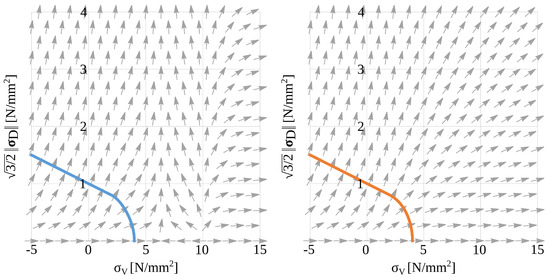
Figure 1. Comparison of the directions of plastic flow with the Drucker–Prager cap model as presented in [19] (left) and with the new model (right) plotted over the respective yield function.

Hence, depending on the stress state and the chosen material parameters, the load step size has to be chosen rather small to ensure the convergence of the stress return algorithm. The cap formulation proposed in [20] holds similar properties. There, the authors try to remedy this problem with the utilisation of a penalty term. In this contribution, a novel and different approach is taken for the yield function (Equation (6)), the tension cap (Equation (8)) and the compression cap (Equation (9)). The yield function with caps is formulated in an additive form instead of the multiplicative approach, it reads

$$f_{mic}({\sigma }_V,{\mathsf{\sigma }}_D,{\kappa }_{mic})=\frac{3}{2}{\mathsf{\sigma }}_D·{\mathsf{\sigma }}_D-(f_1^2({\sigma }_V,{\kappa }_{mic})+f_t\left({\sigma }_V\right)+f_c\left({\sigma }_V\right))\le 0,$$

(6)

with the Drucker–Prager cone

$$f_1({\sigma }_V,{\kappa }_{mic})={\sigma }_0-\alpha {\sigma }_V+h{\kappa }_{mic},$$

(7)

the tension cap

$$f_t\left({\sigma }_V\right)=-H({\sigma }_V-{\sigma }_V^T){({\sigma }_V-{\sigma }_V^T)}^2{\left(\frac{{\sigma }_0-\alpha x_T}{{\sigma }_V^T-\alpha x_T}\right)}^2$$

(8)

and the compression cap

$$f_c\left({\sigma }_V\right)=-H({\sigma }_V^C-{\sigma }_V){({\sigma }_V-{\sigma }_V^C)}^2{\left(\frac{{\sigma }_0-\alpha x_C}{{\sigma }_V^C-\alpha x_C}\right)}^2.$$

(9)

Here, $H\left(x\right)=\frac{1}{2}(1+\mathrm{sign}\left(\mathrm{x}\right))$ denotes the Heaviside function. The shape of the yield function is defined by the cohesive angle $\alpha$, the initial yield stress ${\sigma }_0$, the transition from the Drucker–Prager cone to the tension and compression cap (${\sigma }_V^T$ and ${\sigma }_V^C$) and the yield limits in the fully triaxial state ($x_T$ and $x_C$), cf. Figure 2. For an associated potential flow the flow directions read

$$m_V=\frac{\partial f^{mic}}{\partial {\sigma }_V},{\mathit{m}}_D=\frac{\partial f^{mic}}{\partial {\mathsf{\sigma }}_D}\mathrm{and}{m}_q=\frac{\partial f^{mic}}{\partial q_{mic}}.$$

(10)

Therefore, the evolution of the plastic volumetric and deviatoric strain and the accumulated plastic strain can be defined by the flow rules

$${\dot{\epsilon }}_V^{pl}=\dot{\lambda }{m}_V,{\dot{\mathsf{\epsilon }}}_D^{pl}=\dot{\lambda }{\mathit{m}}_D\mathrm{and}{\dot{\kappa }}_{mic}=\dot{\lambda }{m}_q,$$

(11)

where $\dot{\lambda }$ is the plastic multiplier. For the derivation of the flow directions (Equation (10)), the flow rules (Equation (11)) and the formulation of the stress return algorithm, refer to [25]. In Figure 1 on the right, the flow direction is again plotted as a vector field over ${\sigma }_V$, this time for the new formulation. It can be seen that the flow direction does not reverse anymore with this new formulation, increasing the convergence radius and enabling the utilisation of bigger load steps.

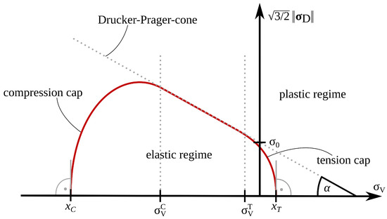
Figure 2. Drucker–Prager cap yield function and the parameters describing it.

2.2. A Discussion of Material Parameter Fitting for the Numerical Model

The fitting of the material model encompasses the elastic material parameters ($K_{mic}$, $G_{mic}$) and the plastic material parameters, namely to describe the yield condition (${\sigma }_0$, $\alpha$, ${\sigma }_V^T$, ${\sigma }_V^C$, $x_T$, $x_C$) and the hardening stiffness (h). The Microplane values connected to the elastic material behaviour are set in relation to the corresponding macroscopic quantities in [19,26]. Thus, the Microplane bulk and shear moduli are set to [26]

$$K_{mic}=\frac{E}{1-2\nu }\mathrm{and}{G}_{mic}=\frac{E}{2(1+\nu )},$$

(12)

respectively. E denotes the macroscopic Young’s modulus and $\nu$ the Poisson’s ratio.

The fitting of the material parameters connected to the plastic material behaviour poses a more complex task. In [19], the uniaxial and biaxial yield stresses are assumed to be directly linked to the yield function on the microscopic level in a manner, which neglects the influence of the different Microplane orientations on the yielding behaviour. Even during initial loading prior to any plasticity effects, the value of ${\mathsf{\sigma }}_D$ is different for every direction, except for a fully volumetric state, such as in triaxial compression or tension. As a result, the yield limit might be reached on different Microplanes at different stages of loading. This leads to a successive plasticising of Microplanes within one material point, which might cause a macroscopic hardening effect even with the assumption of ideal plasticity ($h=0$).

Since the volumetric elastic strains are orientation-independent, ${\sigma }_V$ takes the same value for each direction during initial loading. It will only diverge with the evolution of ${\epsilon }_V^{pl}$ on individual Microplanes. This implies that, for initial loading, the Microplane with ${max}_{i=1,nmp}{\left|\right|{\mathsf{\sigma }}_D\left|\right|}_i$ will first reach the plastic regime, which leads to a redistribution of stresses across all Microplanes in one material point and potentially a much more complex macroscopic stress state. Linking the macroscopic yield stresses to the microscopic yield function therefore requires the consideration of direction.

The macroscopic yield stresses for uniaxial compression and tension, biaxial compression and triaxial compression are denoted ${\sigma }_{yield}^{uc}$, ${\sigma }_{yield}^{ut}$, ${\sigma }_{yield}^{bc}$ and ${\sigma }_{yield}^{tc}$, respectively. As demonstrated in Figure 3 on the right, these quantities indicate the deviation from linear elastic material behaviour and can be obtained from stress–strain curves.

Figure 3. Yield function set into relation with macroscopic yield stresses (left) and exemplary stress–strain plot with these macroscopic yield stresses for uniaxial compression (blue), biaxial compression (orange), triaxial compression (grey) and uniaxial tension (green) (right, not true to scale).

For a uniaxial stress state, the first Microplane plasticising is the one oriented in the direction of the loading, resulting in the microscopic volumetric and deviatoric yield stresses of $-\frac{1}{3}{\sigma }_{yield}^{uc}$ and $\sqrt{\frac{2}{3}}{\sigma }_{yield}^{uc}$ ($\frac{1}{3}{\sigma }_{yield}^{ut}$ and $\sqrt{\frac{2}{3}}{\sigma }_{yield}^{ut}$ for tension). For a biaxial stress state (−1/−1/0), where negative signs indicate compressive loads, it is the one perpendicular to both loading directions. Here, the microscopic yield stresses are $-\frac{2}{3}{\sigma }_{yield}^{bc}$ and $\sqrt{\frac{2}{3}}{\sigma }_{yield}^{bc}$. For a triaxial stress state (−1/−1/−1), all Microplanes will plasticise simultaneously at a microscopic volumetric yield stress of $-{\sigma }_{yield}^{tc}$ since the deviatoric part of the stress tensor vanishes.

With this connection between the first yielding observable in the macroscopic behaviour and the Microplane yielding stresses for different stress states, a first estimate of the geometry of the yield function is possible; see Figure 3 on the left. In [19], it is assumed that the original Drucker–Prager cone, and therefore ${\sigma }_0$ and $\alpha$, is to be determined by the uniaxial and biaxial compressive stress state. This assumption could be checked with the biaxial experiments presented in this paper with different load ratios, cf. Section 4.2. The tension cap (${\sigma }_V^T$, $x_T$) and the compression cap (${\sigma }_V^C$, $x_C$) can be evaluated by means of a uniaxial tension test and the triaxial compression test (−1/−1/−1), respectively. For now, it is assumed that, following [19], ${\sigma }_V^T=-\frac{1}{3}{\sigma }_{yield}^{uc}$ and ${\sigma }_V^C=-\frac{2}{3}{\sigma }_{yield}^{bc}$. This results in

$$\alpha =\frac{\sqrt{6}({\sigma }_{yield}^{bc}-{\sigma }_{yield}^{uc})}{2{\sigma }_{yield}^{bc}-{\sigma }_{yield}^{uc}}\mathrm{and}{\sigma }_0=\sqrt{\frac{2}{3}}{\sigma }_{yield}^{uc}-\frac{\alpha }{3}{\sigma }_{yield}^{uc}.$$

(13)

The hardening stiffness h is to be determined by means of a comparison of simulated and experimentally obtained stress–strain curves. Since the hardening parameter is independent of the Microplane direction, this theoretically can be determined for any and all tests. However, due to the consecutive plasticising of Microplanes and the resulting macroscopic hardening effects, it is reasonable to give an initial prediction for h based on the triaxial compression test, since, as mentioned above, all Microplanes will plasticise at once at those stress states. In further comparisons, this assumption ought to be tested.

Lastly, more experiments, especially cyclic tests and tests with varying load directions, are necessary to validate and elaborate the material parameter fits and the material model. For this, however, damage or fracture effects have to be included in the model, as they were in [19,27,28], for the initial formulation of the yield function and is still part of ongoing research for this specific yield function formulation.

3. Experimental Investigations

3.1. Background

The previous chapter described in detail which material parameters are required for the assumed material model. This material model was developed in the context of the CRC/TRR 280 project [5]. However, for the concretes used in this project no multiaxial tests are available. As mentioned at the beginning, there is little experimental basis for the multiaxial material behaviour of high-strength fine-grained concretes in general. In order to draw conclusions on many of these parameters, similar concretes from other projects have to be considered.

Initial findings were drawn from the DFG-funded project “Experimental Investigation of the Load-bearing Behaviour of Textile Concrete under Uniaxial Compressive Loading—2nd Stage: Influence of Biaxial Loading”. Out of the various high-strength fine-grained concretes that have been developed to meet the requirements of carbon concrete construction, Pagel TF10 [29] was chosen as a representative material. With a characteristic compressive strength of at least $80\mathrm{N}/{\mathrm{mm}}^2$, after 28 days, it is similar to the concretes used within the SFB/TRR 280 project. An initial classification of high-strength fine-grained concretes in the literature will be made on the basis of the biaxial tests carried out on this concrete. In particular, biaxial compressive loading and compressive loading with transverse tensile stress were used. Ideally, the material behaviour should match that of other concretes of the same strength made from standard aggregates. If this is the case, the literature results can be used for initial approximations with the material model, even for those tests not yet performed with fine-grained concretes.

3.2. Experimental Methodology

The analysis of the test results is conducted in two steps. First, the strengths obtained in the two-dimensional stress space are compared with those in the literature. By comparing the strengths, a general statement can be made about the classification of the concrete. For parameter fitting, a more detailed observation of the stress–strain curves is also necessary to draw conclusions about the required parameters shown in Figure 3.

Concrete biaxial strength is usually plotted in a two-dimensional stress space. The stress values (${\sigma }_i$) obtained in each loading direction are related to a reference strength ($f_c^{\prime }$), which is typically the uniaxial compressive strength obtained in the test setup used; see Figure 4. To determine the fracture curve, various loading ratios have to be considered. The load increase in the second load axis is chosen in some proportion to that in the principal compressive direction. As shown in Figure 4, the uniaxial compressive loading (−1/0) and a simultaneous compressive load increase in both load axes (−1/−1) have to be considered for the parameter fitting of the material model. These were also the main support points in determining the fracture curve in the 2D stress space. In addition, the load ratio (−1/−0.5) was investigated, as this shows the maximum strength increase especially for concretes of higher strength [12,13,14,15]. During the parameter fitting, the stress–strain curves of this load ratio can be used to check the material model for stress states that were not specified during the calibration.

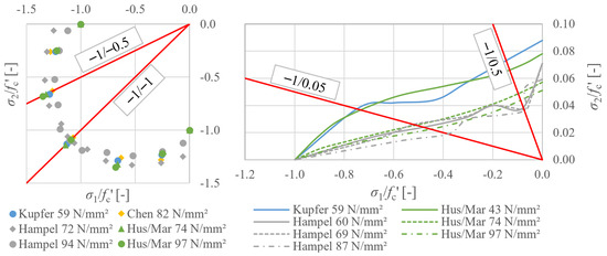
Figure 4. Results in 2D stress space from the literature [12,13,14,15] related to the unconfined compressive strength in the same test setup ((left): biaxial compression; (right): compression-tension loading).

For the combined compressive-tensile loading, the uniaxial tensile strength of the specimens (0/1) had to be investigated. As shown in Figure 4, it has been found in the literature that a large influence on compressive strength already occurs in the range of small tensile loads [12,14,15]. This effect becomes more pronounced at higher compressive strengths due to the proportionally lower tensile strength. To cover this case, the stress ratio (−1/0.05) was considered. In addition, the stress level (−1/0.5), which in the literature often represents a transition point from which the residual compressive strength is approximately at its lowest for high-strength concretes, was investigated.

3.3. Material

The Pagel TF10 is marketed by Pagel Spezial-Beton GmbH & Co. KG and has been developed within the framework of the general technical approval (abZ) “CARBOrefit^®” (formerly TUDALIT) for use in the strengthening of ferro-concrete components with carbon concrete [30]. As defined by the standard [31], this product is a dry mortar with a maximum grain size of $1\mathrm{mm}$. As with other mortars, all the dry components are already packaged in bags, so that only water needs to be added on site. The concrete guarantees a compressive strength of at least $80\mathrm{N}/{\mathrm{mm}}^2$ after 28 days and a modulus of elasticity above 25,000 $\mathrm{N}/{\mathrm{mm}}^2$. The actual concrete properties of the specimens tested are given in the following description of the test results.

3.4. Test Setup

The tests were carried out in the triaxial testing machine (“Triax”) at the Otto Mohr Laboratory of the Dresden University of Technology (see Figure 5 left). This is a single-piece cast steel frame whose high rigidity minimises the mutual influence of the three load axes. It has a compressive capacity of $5000\mathrm{kN}$ and a tensile capacity of $500\mathrm{kN}$. The load is applied by loading brushes, which enable a uniform load application. They consist of several high-strength steel bristles with a yield strength of over $1000\mathrm{N}/{\mathrm{mm}}^2$ that are separated by small gaps (see Figure 5 right). The load in the main compression axis is applied displacement controlled at a speed of $0.003\mathrm{mm}/\mathrm{s}$, and the second load axis is then adjusted force controlled at the desired ratio.

Figure 5. Test setup (left), arrangement of measuring equipment (middle) and specimen placed between the load brushes (right).

The biaxial compression tests were carried out on cubes with an edge length of $100\mathrm{mm}$. This geometry is well known for biaxial compression tests from the literature [12,15,16,17]. These results were then compared with biaxial compression tests previously carried out by other researchers on high-strength concretes [12,13,14,15]. For compressive tests with transversal tensile stresses, disc-shaped specimens are mainly known from the literature [12,14,15]. Based on the experiments by Kupfer [12] and Hampel [15], discs with a base area of $200\times 200{\mathrm{mm}}^2$ were chosen. A thickness of 40 mm was chosen based on realistic component thicknesses of carbon concrete components, e.g., [32]. The tests were predominantly carried out after a minimum of 42 days, as testing after 28 days could not be guaranteed due to the complexity of the testing machine. The Pagel TF10 shows little change in compressive strength after this age [9,33]. An overview of the tested specimens can be found in Table 1. The following plots in two-dimensional stress space show the mean values of the specimens for each loading ratio of the respective geometry. To determine the standard compressive and flexural tensile strength of each batch of concrete, additional prisms measuring $160\times 40\times 40{\mathrm{mm}}^3$ were made in accordance with DIN EN 196-1 [34].

Table 1. Number of test specimens per load ratio.

	Biaxial Compressive Loads			Compressive-Tensile Loads
	−1/0	−1/−0.5	−1/−1	−1/0.05	−1/0.5	0/1
Cubes $(100\times 100\times 100\mathrm{mm})$
Batch 1 (tested after 28 days)	4	4	4	-	-	-
Batch 2 (tested after 43 days)	4	4	4	-	-	-
Discs $(200\times 200\times 40\mathrm{mm})$
Batch 1 (tested after 56 days)	-	-	-	2	2	2
Batch 2 (tested after 63 days)	-	-	-	2	2	2

For strain measurement, a strain gage cross was placed in the centre of each of the two unloaded specimen surfaces and additionally for the disc specimens horizontal and vertical strain gages were placed in the rim area on the two sides offset from each other; see Figure 5 in the middle. This provided two vertical and two horizontal readings for each side, from which total strain averages were calculated. Transverse strains orthogonal to the slice plane were measured with a linear variable displacement transducer (LVDT) fixed with a measuring clamp in the centre of each side of the specimen.

3.5. Biaxial Compressive Strength

The average compressive strength of the prisms from the concrete batches used for the biaxial compression tests was $105.9\mathrm{N}/{\mathrm{mm}}^2$. The uniaxial compression test in the triaxial testing machine gave a strength of $96.7\mathrm{N}/{\mathrm{mm}}^2$, as shown in Table 2. This means that the ratio between the strength of the specimen tested with load brushes and the prism strength tested with rigid load introduction is approximately 0.9. In addition, the prism tests gave a flexural tensile strength of $7.9\mathrm{N}/{\mathrm{mm}}^2$ and a Young’s modulus of approx. 39,250 $\mathrm{N}/{\mathrm{mm}}^2$. The Young’s modulus calculated at $30\%$ of the maximum load in the uniaxial tests was slightly higher at 41,750 $\mathrm{N}/{\mathrm{mm}}^2$, with an average Poisson’s ratio of $0.26$.

Table 2. Material parameters of the fine-grained concrete for biaxial compressive tests.

	Compressive Strength [N/mm2]	Flexural Strength [N/mm2]	Young’s Modulus [N/mm2]	Poisson’s Ratio [-]
Mean value prisms	105.9	7.86	39,250	-
(acc. to EN 196-1 [34])
Batch 1	102.9	6.9	38,750	-
Batch 2	108.9	8.9	39,750	-
Mean value cubes	96.7	-	41,750	0.26
(uniaxial compressive test)
Batch 1	99.6	-	41,250	0.27
Batch 2	93.7	-	42,250	0.24

As shown in Figure 6, an initial classification of the fine-grained concrete in the two-dimensional stress space was made by comparing the biaxial compressive test results with the results from the literature of high-strength concretes subjected to biaxial compressive loading [12,13,14,15]. In this comparison, the strengths obtained were in close agreement with the material behaviour known from the literature, although the strength increases obtained were slightly higher at $14\%$ for the (−1/−1) load ratio and lower at $27\%$ for (−1/−0.5).

Figure 6. Comparison of the results of biaxial compressive loading with the literature [12,13,14,15].

In addition, the stress–strain curves could be compared with those of Hampel [15], who performed tests on concrete of the same compressive strength and, very conveniently for comparison, the same instrument layout. He also used similar load levels; the exact load levels being shown in the corresponding graphs in Figure 7. It should be noted that the exact data for Hampel’s results were not available; the curves were plotted from [15]. In order to improve the clarity of the graph, only the curves for the second batch of the cube tests are displayed. This confirmed the previously observed fairly good agreement in the two-dimensional stress space between the two sets of tests, which differ mainly in the grain size used (Hampel used a maximum grain size of $16\mathrm{mm}$). Similar stiffnesses as well as changes in the shape of the curves were found in each of the three main axes at all load levels.

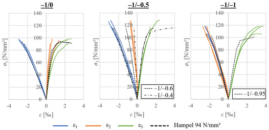
Figure 7. Stress-strain curves of the cubic specimens (batch 2) compared with curves by Hampel [15].

Alongside the increased strength under multi-axial loading, a change in the fracture pattern was observed; see Figure 8. Whereas failure under uniaxial loading was characterised by free crack development, failure under biaxial loading was dominated by splitting in the plane of the two loading directions. This is due to the fact that transverse tensile strains orthogonal to the plane of the disc are mainly possible. The observed behaviour is also consistent with the findings of Hampel [15].

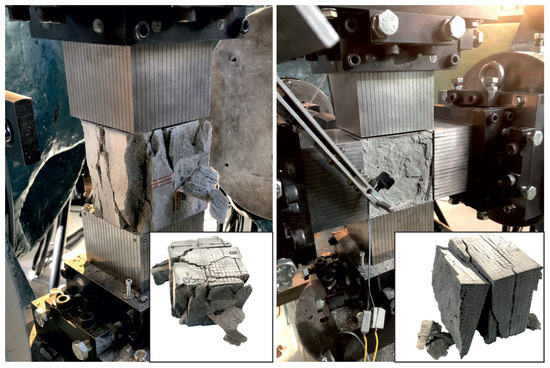
Figure 8. Comparison of a typical fracture pattern with uniaxial (left) and biaxial (right) loading.

3.6. Compressive Strength with Transversal Tensile Stress

The disc specimens for compressive tests with transversal tensile forces were tested around 56 and 63 days after concreting. The specimens were produced in two batches, with two specimens per batch tested at the same tensile loading level; see Table 1. The uniaxial compressive strength of these disc-shaped specimens was previously determined to be $87\%$ of the prism strength [35]. This is in line with the results for the cubic specimens previously mentioned where a ratio of 0.9 was found. Therefore, no additional uniaxial compression tests were performed on the disc specimens. The resulting arithmetic compressive strengths for the discs were determined to be $f_c^{\prime }$ of $88.3\mathrm{N}/{\mathrm{mm}}^2$ and $86.8\mathrm{N}/{\mathrm{mm}}^2$ resulted; see Table 3.

Table 3. Material parameters of the fine-grained concrete for compressive-tensile tests.

	Compressive Strength [N/mm2]	Flexural Strength [N/mm2]	Tensile Strength [N/mm2]	Young’s Modulus [N/mm2]	Poisson’s Ratio [-]
Mean value prisms	100.7	7.76	4.06	-	-
(acc. to EN 196-1 [34])	-	-	-	-	-
Batch 1	101.5	6.84	3.79
Batch 2	99.8	8.68	4.33
Mean value discs	87.6	-	2.79	35,000	0.26
(uniaxial tensile tests)	(calc. 0.87 $f_{c,pr}^{\prime }$)			(tensile)	(tensile)
Batch 1	88.3 (calc.)	-	2.37
Batch 2	86.8 (calc.)	-	3.22

The uniaxial tensile strength $f_t^{\prime }$ of the discs was found to be relatively low at $2.37\mathrm{N}/{\mathrm{mm}}^2$ for the first and $3.22\mathrm{N}/{\mathrm{mm}}^2$ for the second batch. The resulting ratio of the tensile strength to the compressive strength $f_t^{\prime }/f_c^{\prime }$ of $0.032$ ($0.027$ for the first and $0.037$ for the second batch) is significantly lower than previously known for standard concretes. Furthermore, the impact of the size effect [21,36] on the tensile strength is greater than on the compressive strength. Additional tensile tests on prisms of the two batches gave a $f_{t,pr}^{\prime }/f_{c,pr}^{\prime }$-ratio of 0.04.

As mentioned, compared to other concretes, this $f_t^{\prime }/f_c^{\prime }$ -ratio is relatively low; see Figure 9. The ratios for high-strength concretes known from the literature vary between $0.05$ and $0.08$. Under biaxial loading, it is evident that the results for small tensile loads (−1/0.05) resemble very closely the literature results of Hampel [15] and Hussein/Marzouk [14]. At a transverse strain level of ${\sigma }_2/f_c^{\prime }=0.019$, a reduction in compressive strength to $40\%$ was monitored. However, for greater tensile loads (−1/0.5), with a marginally higher transverse strain level of ${\sigma }_2/f_c^{\prime }=0.022$, drastic reductions to just about $5\%$ of the uniaxial compressive strength occur.

Figure 9. Results for combined compressive and tensile loading compared with the literature [14,15].

All specimens failed in the form of a smooth crack as shown in Figure 10. The failure point moved towards the edge of the specimen as the tensile stress level decreased and the compressive stress increased. At (−1/0.05), it could be assumed that the adhesive joint failed as the failure occurred very close to the load application. However, the fracture surface in the lower right image shows that it was the concrete body that failed and not the adhesive joint.

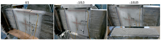
Figure 10. Comparison of a typical fracture pattern with different combined compressive and tensile load paths.

As different batches and geometries are considered here, the stress–strain analysis is relative to the uniaxial strength of the specific specimens. This procedure is well established in the literature [12,14,15]. Unfortunately, the LVDT bracket for measuring strains orthogonal to the plane of the discs did not work on those specimens; therefore, only the results in directions 1 and 2 could be evaluated.

The compressive strain curves in the vertical direction ${\epsilon }_1$ of the uniaxial compression tests and the low transverse strain tests (−1/0.05) show similar stiffness, but failure occurs earlier; see Figure 11 left. As the compressive strength of the Hampel discs is lower this time, the curves deviate somewhat from each other, but the effect of the almost congruent curves for (−1/0) and (−1/0.05) just described is also evident here; see Figure 11 right.

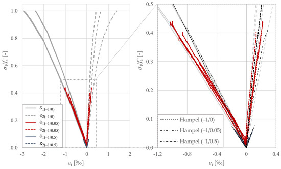
Figure 11. Stress-strain curves of the cubic specimens compared with curves from Hampel [15].

Hampel found a greater reduction in stiffness in the main compression axis in the tests with high transverse tension. This effect, although less pronounced than Hampel’s when compared to the other two curves, can also be seen in our own tests at the load level (−1/0.5). In this load regime, our own curves are almost congruent with Hampel’s but with failure at a lower load level. The curves thus confirm the previously observed effect that at low tensile loads there is relatively good agreement between our own tests and the literature results, but, at higher tensile loads, deviations occur due to the low tensile strength in relation to the compressive strength.

4. Discussion

4.1. Experimental Results

The material behaviour in the biaxial compressive stress space between fine-grained concrete and concretes of similar strength but larger maximum grain size is in good agreement in itself. For verification purposes, a comparison with fracture criteria from the literature is given here. For this purpose, the fracture criteria established in the standard by Kupfer [12] for concretes with a compressive strength greater than $35\mathrm{N}/{\mathrm{mm}}^2$ were used. However, Hampel’s tests showed that these models did not give good agreement for high-strength concretes [15]. He therefore developed his own fracture criterion. These criteria are also used for comparison due to the similarity of the concretes.

It was shown that the Kupfer models gave a fairly good agreement with the test results presented here for fine-grained high-strength concrete, see Figure 12 left. With the Hampel model, however, there is an underestimation of the strength increase, particularly for the design-relevant load path (−1/−1).

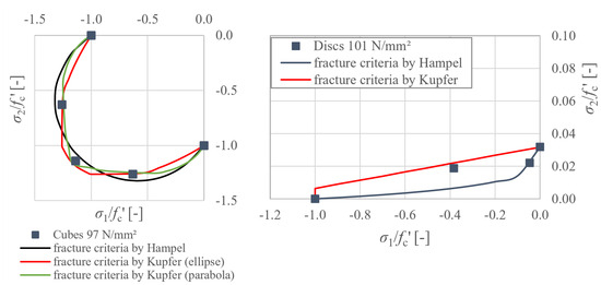
Figure 12. Comparison of the test results with fracture criteria for the 2D stress space from the literature [12,15].

For combined compressive-tensile loading, the fracture criteria from the literature do not fit very well; see Figure 12 right. As seen in the direct comparison above, the ratio of tensile strength to compressive strength is particularly different in the fine-grained concrete compared to the normal grain size concretes. Approximation formulae for tensile strength based on the compressive strength of standard concretes do not work for fine-grained concrete, for which the tensile strength needs to be determined more accurately. For Pagel, the ratio of tensile strength to compressive strength determined with load brushes was $0.032$. Using prisms as a reference, the compressive strength is $0.87f_{c,pr}^{\prime }$. In the compression-tension region, Hampel’s fracture criteria can be used to err on the side of caution by using the actual uniaxial compression–tension stress ratios, but this results in a clear underestimation of the ultimate strength at (−1/0.05). The Kupfer criterion, on the other hand, clearly overestimates the remaining compressive strength at high transverse tensile stresses. Therefore, a new fracture criterion for compressive-tensile loading is recommended for fine-grained concretes.

4.2. Parameter Fitting

As discussed in Section 2.2, some triaxial, biaxial and uniaxial compressive and uniaxial tensile testing is required to reproduce the behaviour of the fine-grained concrete for each stress state. However, as mentioned before, in this publication, only compressive loads can be considered since no damage or fracture model is incorporated in the formulation yet. In the following, the material model is fitted exemplarily via the uniaxial strain–stress curve shown in Figure 7 on the left. Following the argumentation, as presented in Section 3.5, that the biaxial compressive strength increases by $11\%$ compared to the uniaxial compressive strength, the same assumption is made here for the yielding stress. Choosing a uniaxial compressive yield stress of ${\sigma }_{yield}^{uc}=75\mathrm{N}/{\mathrm{mm}}^2$, the biaxial yield stress is therefore ${\sigma }_{yield}^{bc}=83.25\mathrm{N}/{\mathrm{mm}}^2$. With these macroscopic parameters, referring to Section 2.2, the yield function parameters can be calculated. They are given in Table 4, with the exception of the triaxial yield limits $x_T$ and $x_C$. Those were chosen to be $x_T=1\mathrm{N}/{\mathrm{mm}}^2$ and $x_C=-75\mathrm{N}/{\mathrm{mm}}^2$ somewhat arbitrarily and ought to be verified in further research when considering triaxial compression and tension tests. The elastic material parameters are taken from Table 2.

Table 4. Material parameters of the fine-grained concrete for numerical modelling of biaxial tests.

$\mathit{\alpha }$ [-]	${\mathit{\sigma }}_0$ [N/mm2]	${\mathit{\sigma }}_{\mathit{V}}^{\mathit{T}}$ [N/mm2]	${\mathit{\sigma }}_{\mathit{V}}^{\mathit{C}}$ [N/mm2]	h [N/mm2]
0.221	55.716	−25	−55.5	5000

The simulation was carried out in the finite element program feap under the assumption of quasi-static conditions. The loading is applied in a force-controlled manner up to the maximum loads which were observed in the experiments and then the simulation is stopped. It should be mentioned that, since it is reasonable to assume a homogeneous stress state, the discretisation itself is not relevant here. Furthermore, note that since no strain-softening is incorporated into the model, the simulation is not yet able to estimate the maximum force and also not the macroscopic cracking behaviour. The simulated strain–stress curves are depicted in Figure 13 on top of the experimental results. The results for the uniaxial compression test (−1/0) and to biaxial compression tests (−1/−0.5) and (−1/−1) are shown. Here, the ordinate ${\sigma }_1$ refers to the stress in the first principal (loading) direction. For each test, the strains in all three principal directions (${\epsilon }_1$, ${\epsilon }_2$ and ${\epsilon }_3$) are plotted. It can be seen that the model is able to not only capture the (−1/0) test but also is able to predict the material behaviour under the biaxial compressive loads of (−1/−0.5) and (−1/−1) in the principal directions experiencing negative (compressive) strains. However, the model is not quite able to fit the positive (tensile) lateral strain outside of the elastic regime in the third direction. This might be partly due to the mentioned missing strain-softening formulation. However, beyond that, the different results for the transversal directions in the uniaxial compression test would suggest an influence of the two different measuring procedures (c.p. Section 3.4) on the result. Considering this, the choice of the yielding stresses and the assumptions of the relation between macroscopic measurable material parameters and their Microplane counterparts (cf. Section 2.2), especially for the calculation of $\alpha$ and ${\sigma }_0$, therefore seem reasonable.

Figure 13. Comparison of the numerical results with the experimental results for biaxial compression tests of cube batch 2.

Note that, with a positive $\alpha$, one could argue that dilatancy effects are somewhat taken into account within the material model, and the match of the numerical result and the experimental data may suggest that dilatancy effects are reproduced adequately. However, it is necessary to specify this statement with an additional targeted numerical and experimental investigation, for which the required tests are not yet available for fine-grained high-strength concrete. Hence, in this contribution, the topic is left out, though it is an important topic regarding the multiaxial behaviour of concrete. For a more detailed overview, refer to [37], who present an in-depth discussion of the different dilatancy measures and to [38] for a comparison of different Drucker–Prager plasticity models with respect to dilatancy effects.

5. Conclusions

In general, it can be assumed that the multiaxial load-bearing behaviour of the fine-grained concretes is similar to that of the conventional concretes with similar compressive strengths. The tensile strength is lower for the fine-grained concretes relative to the compressive strength than for the normal concretes. This is the main reason for the deviations from the results reported in the literature.

As long as the uniaxial compressive and tensile strengths and the modulus of elasticity are known, the calibration of material models for fine-grained concretes based on literature results for concretes with similar strength values is possible. Increases and decreases in strength under multiaxial loading should be represented sufficiently accurately. This is particularly relevant as a large number of fine-grained concretes have been and are being developed for use in carbon concrete, for which multi-axial tests are often not yet available.

If fracture criteria are introduced in the future, Kupfers’s biaxial compressive stress criteria [11,12] can be used, but, for compressive-tensile stress, a new criterion should be defined to make better use of the material.

Furthermore, a Microplane plasticity material model with Drucker–Prager cap yield function for plain concrete has been introduced. For now, it has been fitted to the biaxial compressive behaviour of the high-strength fine-grained concrete. The macroscopic yield stresses were successfully related to the required model parameters to match the macroscopic concrete behaviour. As a next step, based on the investigation presented in this contribution, already existing experimental data of the multiaxial behaviour of high-strength normal-grained concrete will be utilised for a more comprehensive parameter fit. Additionally, the model needs to be extended to be able to account for material softening.

References

- Triantafillou, T.C. Textile Fibre Composites in Civil Engineering; Woodhead Publishing: Sawston, UK, 2016. [Google Scholar] [CrossRef]
- Spelter, A.; Bergmann, S.; Bielak, J.; Hegger, J. Long-Term Durability of Carbon-Reinforced Concrete: An Overview and Experimental Investigations. Appl. Sci. 2019, 9, 1651. [Google Scholar] [CrossRef]
- Valeri, P.; Guaita, P.; Baur, R.; Fernández Ruiz, M.; Fernández-Ordóñez, D.; Muttoni, A. Textile reinforced concrete for sustainable structures: Future perspectives and application to a prototype pavilion. Struct. Concr. 2020, 21, 2251–2267. [Google Scholar] [CrossRef]
- Giese, J.; Beckmann, B.; Schladitz, F.; Marx, S.; Curbach, M. Effect of Load Eccentricity on CRC Structures with Different Slenderness Ratios Subjected to Axial Compression. Buildings 2023, 13, 2489. [Google Scholar] [CrossRef]
- Beckmann, B.; Bielak, J.; Bosbach, S.; Scheerer, S.; Schmidt, C.; Hegger, J.; Curbach, M. Collaborative research on carbon reinforced concrete structures in the CRC/TRR 280 project. Civ. Eng. Des. 2021, 3, 99–109. [Google Scholar] [CrossRef]
- Lieboldt, M. Feinbetonmatrix für Textilbeton: Anforderungen—baupraktische Adaption—Eigenschaften. Beton- und Stahlbetonbau 2015, 110, 22–28. [Google Scholar] [CrossRef]
- Brockmann, T. Mechanical and Fracture Mechanical Properties of Fine Grained Concrete for Textile Reinforced Composites. Ph.D. Dissertation, RWTH Aachen University, Aachen, Germany, 2006. [Google Scholar]
- Bochmann, J.; Jesse, F.; Curbach, M. Experimental Determination of the Stress-Strain Relation of Fine Grained Concrete under Compression. In Proceedings of 11th HPC and 2nd CIC Conference, Tromso, Norway, 6–7 March 2017; Paper No. 6; Justnes, H., Martius-Hammer, T.A., Eds.; Norwegian Concrete Association/Tekna: Oslo, Norway, 2017. [Google Scholar]
- Bochmann, J. Carbonbeton unter Einaxialer Druckbeanspruchung. Ph.D. Dissertation, Technische Universität Dresden, Dresden, Germany, 2019. [Google Scholar]
- Bosbach, S.; Bielak, J.; Schmidt, C.; Hegger, J.; Claßen, M. Influence of Transverse Tension on the Compressive Strength of Carbon Reinforced Concrete. In Proceedings of the 11th International Conference on Fiber-Reinforced Polymer (FRP) Composites in Civil Engineering (CICE 2023), Rio de Janeiro, Brazil, 24–26 July 2023. Paper 328. [Google Scholar] [CrossRef]
- Kupfer, H. Das Verhalten des Betons unter Zweiachsiger Beanspruchung. Wiss. Z. Tech. Univ. Dresd. 1968, 17, 1515–1518. [Google Scholar]
- Kupfer, H. Das Verhalten des Betons unter Mehrachsiger Kurzzeitbelastung unter Besonderer Berücksichtigung der Zweiachsigen Beanspruchung. In Schriftreihe des DAfStb; Deutscher Ausschuss für Stahlbeton: Berlin, Germany, 1973; Volume 229. [Google Scholar]
- Chen, R.L. Behavior of High-Strength Concrete in Biaxial Compression. Ph.D. Dissertation, University of Texas, Austin, TX, USA, 1984. [Google Scholar]
- Hussein, A.; Marzouk, H. Behavior of High-Strength Concrete under Biaxial Loading. ACI Mater. J. 2000, 97, 27–36. [Google Scholar]
- Hampel, T. Experimentelle Analyse des Tragverhaltens von Hochleistungsbeton unter Mehraxialer Beanspruchung. Ph.D. Dissertation, TU Dresden, Dresden, Germany, 2006. [Google Scholar]
- Speck, K. Beton unter Mehraxialer Belastung—Ein Materialgesetz für Hochleistungsbetone unter Kurzzeitbelastung. Ph.D. Dissertation, TU Dresden, Dresden, Germany, 2007. [Google Scholar]
- Hampel, T.; Speck, K.; Scheerer, S.; Ritter, R.; Curbach, M. High-Performance Concrete under Biaxial and Triaxial Loads. J. Eng. Mech. 2009, 135, 1274–1280. [Google Scholar] [CrossRef]
- Bazant, Z.P.; Oh, B.H. Microplane model for fracture analysis of concrete structures. In Proceedings of the Symposium on the Interaction of Non-Nuclear Munitions with Structures, Colorado Springs, CO, USA, 10–13 May 1983; pp. 49–53. [Google Scholar]
- Zreid, I.; Kaliske, M. A gradient enhanced plasticity–damage microplane model for concrete. Comput. Mech. 2018, 62, 1239–1257. [Google Scholar] [CrossRef]
- Fuchs, E.; Kaliske, M. A gradient enhanced viscoplasticity-damage microplane model for concrete at static and transient loading. In Proceedings of the 10th International Conference on Fracture Mechanics of Concrete and Concrete Structures, Bayonne, France, 23–26 June 2019; pp. 23–26. [Google Scholar] [CrossRef]
- Bazant, Z.P.; Planas, J. Fracture and Size Effect in Concrete and Other Quasibrittle Materials; Routledge: New York, NY, USA, 2019; (print version published 1998). [Google Scholar] [CrossRef]
- Carol, I.; Jirásek, M.; Bažant, Z. A thermodynamically consistent approach to microplane theory. Part I. Free energy and consistent microplane stresses. Int. J. Solids Struct. 2001, 38, 2921–2931. [Google Scholar] [CrossRef]
- Bažant, P.; Oh, B. Efficient numerical integration on the surface of a sphere. ZAMM-J. Appl. Math. Mech. Für Angew. Math. Und Mech. 1986, 66, 37–49. [Google Scholar] [CrossRef]
- Zreid, I.; Kaliske, M. An implicit gradient formulation for microplane Drucker-Prager plasticity. Int. J. Plast. 2016, 83, 252–272. [Google Scholar] [CrossRef]
- Wriggers, P. Nonlinear Finite Element Methods; Springer Science & Business Media: Berlin/Heidelberg, Germany, 2008. [Google Scholar] [CrossRef]
- Leukart, M.; Ramm, E. Identification and interpretation of microplane material laws. J. Eng. Mech. 2006, 132, 295–305. [Google Scholar] [CrossRef]
- Qinami, A.; Pandolfi, A.; Kaliske, M. Variational eigenerosion for rate-dependent plasticity in concrete modeling at small strain. Int. J. Numer. Methods Eng. 2020, 121, 1388–1409. [Google Scholar] [CrossRef]
- Platen, J.; Zreid, I.; Kaliske, M. A nonlocal microplane approach to model textile reinforced concrete at finite deformations. Int. J. Solids Struct. 2023, 267, 112151. [Google Scholar] [CrossRef]
- Pagel Spezial-Beton GmbH & Co. KG. Datenblatt Pagel TF10 CARBOrefit® Textilfeinbeton; Pagel Spezial-Beton GmbH & Co. KG: Essen, Germany, 2022. [Google Scholar]
- Deutsches Institut für Bautechnik. CARBOrefit®—Verfahren zur Verstärkung von Stahlbeton mit Carbonbeton: Allgemeine Bauaufsichtliche Zulassung (abZ)/Allgemeine Bauartgenehmigung (aBG) Z-31.10-182; Deutsches Institut für Bautechnik: Berlin, Germany, 2021. [Google Scholar]
- DIN EN 206:2013+A2:2021; Concrete—Specification, Performance, Production and Conformity. Beuth-Verlag: Berlin, Germany, 2021.
- Frenzel, M.; Tietze, M.; Curbach, M. C3 Technology Demonstration House—CUBE: Design and Manufacturing of the Twisted Roof-Wall Construction. In Proceedings of the 6th fib International Congress, Oslo, Norway, 12–16 June 2022; pp. 2542–2550. [Google Scholar]
- Hering, M. Untersuchung von Mineralisch Gebundenen Verstärkungsschichten für Stahlbetonplatten gegen Impaktbeanspruchungen. Ph.D. Dissertation, Technische Universität Dresden, Dresden, Germany, 2020. [Google Scholar]
- DIN EN 196-1:2016; Methods of Testing Cement—Part 1: Determination of Strength. Beuth-Verlag: Berlin, Germany, 2016.
- Betz, P.; Marx, S.; Curbach, M. Einfluss von Querzugspannungen auf die Druckfestigkeit von Carbonbeton. Beton- und Stahlbetonbau 2023, 118, 524–533. [Google Scholar] [CrossRef]
- Bazant, Z.P. Size effect on structural strength: A review. Arch. Appl. Mech. 1999, 69, 703–725. [Google Scholar]
- Wosatko, A.; Winnicki, A.; Polak, M.A.; Pamin, J. Role of dilatancy angle in plasticity-based models of concrete. Arch. Civ. Mech. Eng. 2019, 19, 1268–1283. [Google Scholar] [CrossRef]
- Yu, T.; Teng, J.; Wong, Y.; Dong, S. Finite element modeling of confined concrete-I: Drucker–Prager type plasticity model. Eng. Struct. 2010, 32, 665–679. [Google Scholar] [CrossRef]
Disclaimer/Publisher’s Note: The statements, opinions and data contained in all publications are solely those of the individual author(s) and contributor(s) and not of MDPI and/or the editor(s). MDPI and/or the editor(s) disclaim responsibility for any injury to people or property resulting from any ideas, methods, instructions or products referred to in the content. |
© 2023 by the authors. Licensee MDPI, Basel, Switzerland. This article is an open access article distributed under the terms and conditions of the Creative Commons Attribution (CC BY) license (https://creativecommons.org/licenses/by/4.0/).