Data-Driven Prediction Model for High-Strength Bolts in Composite Beams

Abstract

In recent years, the application of artificial intelligence-based methods to engineering problems has received consistent praise for their high predictive accuracy. This paper utilizes a BP neural network to predict the strength of steel–concrete composite beam shear connectors with high-strength friction-grip bolts (HSFGBs). These connectors are widely used in bridge and building construction due to their superior strength and stiffness compared to traditional beams. A validated finite element model was used to predict the strength of HSFGB shear connectors. A reliable database was created by analyzing 208 models with different characteristics for machine learning modeling. Previous studies have identified issues with result variation and overestimation or underestimation of shear connection strength. Among the machine learning methods evaluated, the backpropagation neural network model performed the best. It achieved a goodness of fit of over 93% in both the training and testing sets, with a low coefficient of variation of 6.50%. Concrete strength, bolt diameter, and bolt tensile strength were found to be important variables influencing the strength of shear connectors. Other variables showed a proportional or inverse relationship with compressive strength, except for concrete strength and bolt pretension. This study presents an accurate machine learning approach for predicting the strength of HSFGB shear connectors in steel–concrete composite beams. The study offers valuable insights into the effects of various variables on the performance of shear connection strength, providing support for structural design and analysis.

1. Introduction

In recent years, there has been a substantial increase in the use of steel–concrete composite beams in bridges and buildings. These composite beams provide several advantages compared to pure steel or concrete beams, such as superior initial stiffness and strength, a higher span-to-depth ratio, and reduced mid-span deflection, as demonstrated in Figure 1. As a result, they have been widely adopted in construction projects. Shear connectors play a crucial role in facilitating the transfer of forces between the steel beam and the concrete slab in steel–concrete composite beams. The most commonly used shear connectors are headed stud connectors, which are welded to ensure a strong and ductile shear connection. However, due to an increasing focus on recycling, there is a need for more sustainable installation techniques. High-strength friction-grip bolt (HSFGB) shear connectors have emerged as a viable alternative in response to this need. These connectors not only require the tightening of nuts but also provide easier recyclability, making them highly suitable for future development and construction projects.

During the 1970s, Marshall et al. [1] conducted a series of experimental studies to investigate the application of high-strength friction-grip bolts (HSFGBs) as shear connectors in steel–concrete composite structures. Recently, Kwon et al. [2] conducted tests on three types of post-installed shear connectors under static and fatigue loads, aiming to investigate methods for achieving composite action in existing non-composite bridges. Pathirana et al. [3] performed composite beam tests using blind bolts and welding studs, and their findings demonstrated that blind bolts are a more reliable method than welding studs for achieving and maintaining composite action. Zhang et al. [4] conducted 11 sets of experimental studies on the static performance of HSFGB shear connectors in composite beams and proposed a formula for predicting the ultimate strength of these connectors. However, early models often lacked sufficient experimental data, resulting in limited effectiveness in predicting the ultimate strength of HSFGB shear connectors. Therefore, it becomes crucial to develop a prediction formula that is accurate and reliable by utilizing extensive experimental data and considering multiple variables.

Recently, there has been a growing popularity in the use of machine learning techniques for predicting the structural state. These AI techniques have demonstrated promising results in modeling and predicting behaviors in civil engineering problems [5,6,7,8,9,10,11]. In the field of structural engineering, machine learning has proven to be precise and reliable. Tohidi and Sharifi successfully developed a backpropagation neural network that accurately predicts the residual flexural strength of corroded steel plate beams [12]. In a separate study, Sharifi et al. investigated the use of neural network models to predict the ultimate bearing capacity of honeycomb steel beams. They conducted tests with different learning algorithms and hidden neuron configurations to determine the most effective network. Additionally, they introduced a novel formula that utilizes artificial neural networks to estimate the failure load of honeycomb steel beams [13]. Sarothi et al. performed a comprehensive comparison of various machine learning models, such as linear regression, ridge regression, lasso regression, support vector machine, decision tree, random forest, k-nearest neighbors, artificial neural networks, XGBoost, AdaBoost, and CatBoost. They trained and evaluated a total of 11 models for predicting the shear bolt connection capacity. The results indicated that the random forest model outperformed the others in terms of predictive performance. Moreover, they presented a formula derived from this model [14]. Bagherzadeh et al. developed a high-precision computational model by integrating multiple machine learning tools to predict the maximum tensile stress of a plain-woven composite panel with two interacting grooves. The model incorporates GBR, PolyFeatures, and LassoLarsCV algorithms, outperforming other machine learning combinations and artificial neural networks in predicting the target values [15]. Asgarkhani et al. enhanced ML algorithms using a pipeline-based hyper-parameter fine-tuning method and feature selection techniques to prevent overfitting and data leakage. The results indicate that the proposed methods achieve high prediction accuracy (over 95%) and curve fitting ability, enabling the estimation of the median of the IDA curve and the seismic failure probability curve for an accelerated seismic risk assessment [16]. Hosseinpour employed neural networks to predict the ultimate strength of bolt shear connectors in composite cold-formed steel beams. The study specifically examined grade 8.8 bolt shear connectors and offered a formula to accurately determine their ultimate strength [17]. Collectively, these studies have conclusively demonstrated the feasibility and effectiveness of utilizing machine learning approaches in the field of structural engineering.

Therefore, a finite element model was established to investigate the static performance of high-strength bolted connections in composite beams. Xing’s experimental results [18] were utilized to validate these models. Figure 2 illustrates the exact measurements and configurations. Subsequently, a thorough analysis was conducted, consisting of 144 finite element models that accounted for different factors impacting the maximum shear strength of bolted connections. Utilizing the insights gained from this analysis, an operational correlation using artificial neural networks was developed to predict the ultimate shear strength of high-strength bolted connections. The database obtained from the analysis was employed to supply input and target data for the neural network. Additionally, to obtain more accurate prediction formulas, five methods were compared as follows: linear regression (ridge regression and ordinary least squares) and nonlinear regression (decision trees, random forests, and backpropagation neural networks). The results indicated that the backpropagation neural network method is most suitable for predicting the ultimate shear strength of HSFGB bolted connections in composite beams. By comparing the calculated values of the proposed formula with those obtained from the relevant literature, it was demonstrated that the proposed formula can provide reasonable prediction results.

2. Finite Element Modeling

For machine learning, having more data is generally better; in most cases, having more data can provide better training results. Larger datasets can help models capture patterns and regularities in the data, thereby improving their generalization ability. However, we currently only have 64 sets of experimental data, so we must build additional validated finite element models to supplement our database. ABAQUS 2023 is a popular and versatile software used for finite element analysis in mechanical engineering [19]. It offers a wide range of features and analysis options, allowing engineers and researchers to simulate and analyze various engineering applications. These include static and dynamic analysis, linear and nonlinear material models, and more. ABAQUS is known for its powerful modeling and post-processing capabilities, making it a valuable tool for addressing complex engineering problems. That is why we have chosen ABAQUS as our preferred finite element analysis software.

2.1. Material Constitutive

2.1.1. Concrete

The concrete material constitutive model employed in this study was proposed by Ding et al. [20] and is as follows:

$$y=\left\{\begin{array}{c}\frac{A_{n}x+\left(B_n-1\right)x^2}{1+\left(A_n-2\right)x+B_n{x}^2},x\le 1\\ \frac{x}{{\alpha }_n{\left(x-1\right)}^2+x},x>1\end{array}\right.$$

(1)

where $A_n$ represents the ratio of the initial tangent modulus to the secant modulus at the point of peak stress, and the initial tangent modulus equates to the elastic modulus. $B_n$ is a parameter that regulates the reduction in the elastic modulus during the upward segment of the axial stress–strain correlation. The proposed elastic modulus (${\mathrm{E}}_{\mathrm{c}}$) values for different strength grades of concrete are as follows:

$${\mathrm{E}}_{\mathrm{c}}=9500{{\mathrm{f}}_{\mathrm{c}\mathrm{u}}}^{1/3}$$

(2)

$$\begin{gathered} f_c={0.4f_{cu}}^{7/6}; \\ \mathrm{Or}{f}_t={0.24f_{cu}}^{2/3}. \end{gathered}$$

(3)

$$\begin{gathered} {\epsilon }_c={383f_{cu}}^{7/18}\times {10}^{-6}; \\ \mathrm{Or}{\epsilon }_t={33f_{cu}}^{1/3}\times {10}^{-6}. \end{gathered}$$

(4)

• In the case of concrete under compression, the following definitions apply: $y$ represents the ratio of the compressive stress ($\sigma$) to the uniaxial compressive strength ($f_c$), x denotes the ratio of the compressive strain ($\epsilon$) to the corresponding compressive strain at the uniaxial tensile strength (${ϵ}_c$), and $n$ is set to 1. The variables $f_c$ and $f_t$ stand for the uniaxial compressive and tensile strengths of concrete, respectively, while ${ϵ}_c$ and ${\epsilon }_t$ are the associated compressive and tensile strains. Additionally, $f_{cu}$ represents the compressive cubic strength of concrete, with the variables $A_1$ and $B_1$ defined as $A_1=9.1{f_{cu}}^{-4/9}$ and $B_1=1.6{\left(A_1-1\right)}^2$, respectively. For overall concrete, ${\alpha }_1$ is given as $2.5\times {10}^{-5}{f_{cu}}^3$, while ${\alpha }_1=0.15$ is used for locally confined concrete in the nonlinear finite element analysis.
• For concrete in tension, the following relationships are established: y is the ratio of the tensile stress ($\sigma$) to the uniaxial tensile strength ($f_t$), x represents the ratio of the tensile strain ($\epsilon$) to the corresponding tensile strain at the uniaxial tensile strength (${ϵ}_t$), and $n$ is set to 2. The variable $A_2$ is assigned a value of 0.8 for the nonlinear finite element analysis of reinforced concrete structures, while $B_2$ is calculated as $5{\left(A_2-1\right)}^2/3$. Additionally, ${\alpha }_2$ equals $1+3{f_{cu}}^2\times {10}^{-4}$.

2.1.2. Steel Components

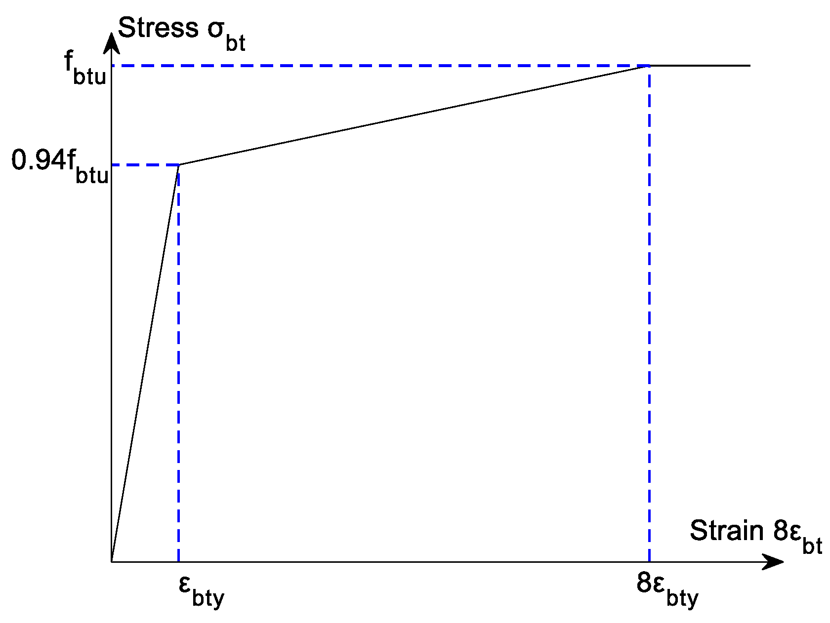
In this study, we utilized a tri-linear constitutive model, which was suggested by Loh et al. [21], to accurately simulate the characteristics of high-strength bolt materials. This model is visually depicted in Figure 3. In this model, the ultimate strength (${\mathrm{f}}_{\mathrm{b}\mathrm{t}\mathrm{u}}$) and yield strain (${\mathsf{\epsilon }}_{\mathrm{b}\mathrm{t}\mathrm{y}}$) were used, with the ultimate strain set at 8${\mathsf{\epsilon }}_{\mathrm{b}\mathrm{t}\mathrm{y}}$. To verify and analyze the model, we adopted a bolt fracture strain of 0.15, as suggested by Shi et al. [22]. The adopted failure criterion is “Ductile Damage”. For the simulation of steel beams, gaskets, and reinforced bars, an ideal elastic–plastic constitutive model was used, neglecting the strain-hardening phenomenon. The steel material was characterized by an elastic modulus of 205 GPa and a Poisson’s ratio of 0.3. The yield strengths of the steel beam, gaskets, and reinforced bars were 353 MPa, 1150 MPa, and 340 MPa, respectively. The diameter of the steel reinforcement was assumed to be Φ10, and the specific values align with the experimental data mentioned in the literature. For more detailed information, please refer to

Table 1. Details of test specimens and failure mode.

Specimen	Concrete Strength ${\mathit{f}}_{\mathit{c}\mathit{u}}$ (MPa)	Bolt $\mathbf{Diameter}\mathit{d}$ (mm)	$\mathbf{Ultimate}\mathbf{Strength}{\mathit{f}}_{\mathit{u}}$ (MPa)	Bolt Pretension $\mathit{T}$ (kN)	Preformed Hole Diameter		Failure Mode
					Concrete Slab (mm)	Steel Flange (mm)
PT1	45.6	16	1083	80.7	20	18	B.F.
PT2	60.2	16	1303	101.2	20	18	B.F.
PT3	74.8	20	1024	126.4	24	22	B.F.
PT4	61.6	16	1083	77.3	20	18	B.F.
PT5	73.1	22	990	76.3	26	24	B.F.
PT6	68.9	20	1024	77.9	24	22	B.F.

B.F. = Bolt failure.

.

2.2. Geometric Model, Element Type, and Mesh

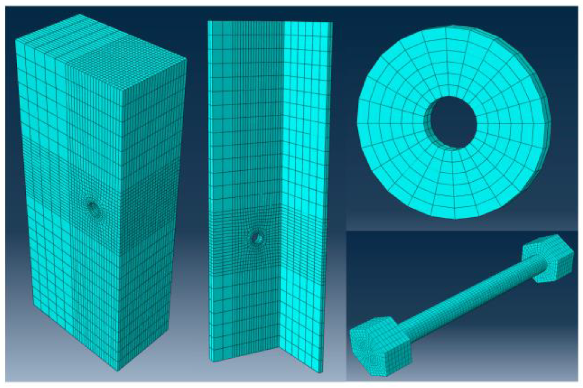
The specific grid size is depicted in Figure 4. To strike a balance between computational speed and accuracy, a grid sensitivity analysis was conducted. The grid sizes chosen at this point not only ensure computational efficiency but also maintain a high level of accuracy. The bolts, steel gaskets, and rigid base were divided into grids using the global seeding method with grid sizes of 2.5 mm, 6 mm, and 50 mm, respectively. The reinforcement bars were divided into grids using the local seeding method with a grid size of “1”. The steel beam had the following three levels of mesh sizes: an overall size (20 mm), a size around the holes (5 mm), and a size along the innermost circumference of the holes (2.5 mm). The concrete slab had the following three levels of mesh sizes: an overall size (20 mm), a size around the holes (5 mm), and a size along the inner-layer circumference of the holes (2.5 mm). Notably, for thin-walled components, it is advisable to utilize local seeding and incorporate two or more layers of grids to enhance analysis precision and stability. In this study, a two-layer grid system was utilized. Regarding the clearance between the bolt and the hole in different components, the actual assembly conditions were taken into consideration. A 1 mm clearance was considered for the steel gaskets, a 2 mm clearance for the steel beam flanges, and a 4 mm clearance for the precast concrete slabs. This ensured a more accurate representation of the physical assembly conditions.

To ensure an accurate simulation of the structural behavior, we carefully selected the appropriate element types for each component. Additionally, we made necessary revisions to enhance the accuracy of the simulation. The two-node three-dimensional truss element (T3D2) was chosen to model the reinforced bars embedded in the concrete slab, taking into consideration the geometrical symmetry of the specimens and specified boundary conditions. For all other structural components, except for the reinforcing bars, the eight-node linear hexahedral solid element (C3D8R) was utilized. The C3D8R element is widely used in engineering due to its numerous advantages, including high precision, geometric flexibility, numerical stability, and a wide range of applications. This selection of element types ensured an accurate and reliable simulation of structural behavior.

2.3. Interaction Conditions

The contact between surfaces was simulated using a face-to-face contact model, which allows for separation between the surfaces while preventing penetration. To characterize the frictional behavior, a friction coefficient of 0.52 was assigned to the interfaces between steel and concrete. This value was determined based on the average obtained from the interface friction values reported by Rabbat et al. [23] and Guo et al. [24]. In addition, a friction coefficient of 0.25 was applied to all steel interfaces. To account for the interaction and connection between the concrete slab and the reinforced bars, embedded constraints were implemented. The “Embedded Region” command was utilized to embed the steel reinforcement within the concrete elements. This approach ensures a realistic representation of their mutual influence and connection.

2.4. Boundary Conditions

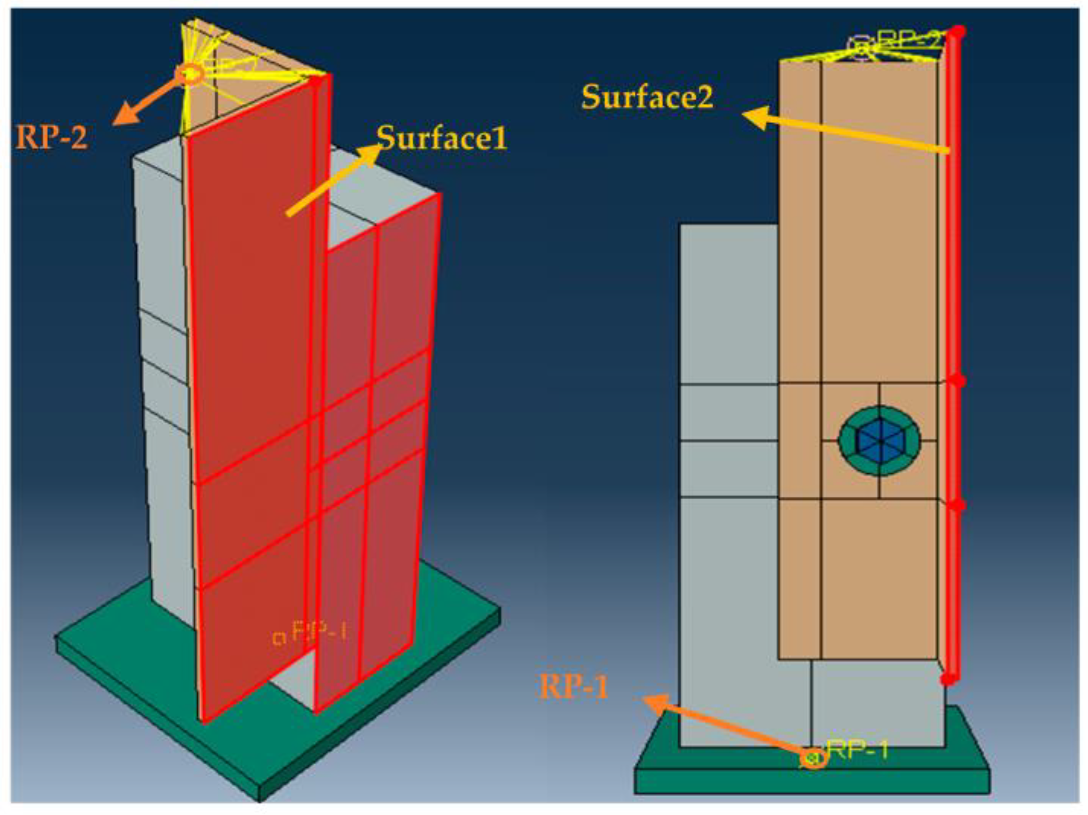
To accurately capture the experimental conditions, a rigid constraint is applied to the steel footing. The center of the bottom surface serves as the constraint point (RP-1), where a fixed constraint is imposed to prevent any movement. For the surface 1 and surface 2 of the model, symmetric boundary conditions are applied to ensure symmetry and balance in the analysis. To constrain the top surface, a structural coupling approach is employed. It is coupled at the point (RP-2), as depicted in Figure 5. This coupling ensures that the top surface remains constrained and properly connected to the surrounding components.

2.5. Loading, Analysis Method, and Failure Criteria

The nonlinear problem is addressed through the utilization of the general static analysis method in ABAQUS. The loadings consist of bolt preloading and external loads, which are divided into two analysis steps for accurate simulation. In the first step, the “Bolt Load” functionality within the statics module is employed to apply the preload to the bolts. This step ensures that the bolts are properly preloaded before subjecting the structure to external loading. In the second step, a downward displacement load is applied at the coupling point on the top surface. To maintain equilibrium and account for the interaction between the bolt preload and the externally applied load, the bolt force control mode is modified to “Fixed at Current Length”. This adjustment allows the preload on the bolt to vary accordingly with the applied load, ensuring the structure remains in a state of balance and stability throughout the analysis.

The model can experience three potential failure modes. The first mode is associated with the steel beam, wherein the local strain and stress exceed their respective limits, resulting in a loss of normal working capacity. For the concrete slab, the second failure mode occurs when the strain and damage surpass the specified limits under tension or compression. These criteria act as indicators for potential cracking or fracturing. The third failure mode involves the bolt rod section near the interface between the steel beam and concrete slab. If the strain and stress in this region reach the anticipated fracture strain and tensile strength, it will lead to bolt failure. The predominant failure modes observed, based on available tests, are related to the concrete slab and the bolt rod section. Specifically, the second failure mode pertains to the concrete slab, while the third failure mode is associated with the bolt rod section. These findings are derived from extensive testing.

2.6. Finite Element Model Verification

We verified the accuracy of the finite element analysis by conducting a comparison with experimental results, as shown in

Table 2. Comparisons of the testing with predictions.

Test		PT1	PT2	PT3	PT4	PT5	PT6	Average	Standard Deviation
	T	142.4	168.4	257.1	158.3	266.1	240.3
	FEA	148.6	175.2	242.1	154.3	268.4	230.6
	T/FEA	0.96	0.96	1.06	1.03	0.99	1.04
	FEFM	B.F.	B.F.	B.F.	B.F.	B.F.	B.F.
								1.01	0.04

T = test, FEA = finite element analysis, FEFM = finite element failure mode, B.F. = bolt failure.

. This validation process ensured the reliability and precision of our analysis. The simulated results from the analysis closely matched the experimental data, with an average ratio of approximately 1.01. The standard deviation between the simulated and experimental results was only 0.04, indicating a strong agreement. Notably, the finite element model accurately predicted the observed failure mode in the experiments. These findings support the reliability of the finite element model for data analysis and future investigations. The slight discrepancies may be attributed to the inherent experimental errors and the inaccuracies in the material constitutive models used in the finite element simulation. For a detailed visual representation, please refer to Figure 6.

3. Establishment of a Database

3.1. Choosing Research Variables

The prevailing approach for enhancing the accuracy of HSFGB shear connectors’ ultimate strength prediction involves refining the formulas introduced in EN1994-1-1 [25] that pertain to the ultimate strength of shear connectors with headed studs.

$$\begin{gathered} P_{u,c}=\raisebox{1ex}{$0.8f_u\mathsf{\pi }{d}^2/4$}\!\left/ \!\raisebox{-1ex}{${\gamma }_v$}\right., \\ \mathrm{Or}{P}_{u,c}=\raisebox{1ex}{$0.29\alpha d^2\sqrt{f_{ck}{E}_c}$}\!\left/ \!\raisebox{-1ex}{${\gamma }_v$}\right. \end{gathered}$$

(5)

where:

• ${\gamma }_v$ = 1.25 is the partial factor.
• d is the diameter of the shank of the stud.
• $h_{sc}$ is the overall nominal height of the stud.
• $\alpha =0.2(h_{sc}/d+1)$ for $3\le h_{sc}/d\le 4$; $\alpha =1$ for $hsc/d>4$.
• $f_u$ is the specified ultimate tensile strength of the material of the stud.
• $f_{ck}$ is the characteristic cylinder compressive strength of the concrete at the age considered.

Due to the nature of the HSFGB being studied, $\alpha$ is usually set to 1. Additionally, according to Formulas (2) and (3), mentioned in Ding et al. [20], $E_c$ and $f_{ck}$ can be related to the compressive strength of standard concrete cubes. Therefore, based on Formula (5), the characteristics of high-strength frictional shear connectors, relevant experiments conducted by researchers, and the availability of data, the variables considered in this study are the compressive strength of standard concrete cubes (GB50010) (150 mm × 150 mm × 150 mm) [26], the diameter of the connecting rod, the ultimate tensile strength of the shear connector, the nominal hole diameter in concrete, and the pretension force of the bolt.

3.2. Data Collection Standards and Guidelines

The following criteria outline the standards for data collection:

• To apply forces, all specimens are loaded using the method of “inserting a steel beam between two concrete slabs”.
• The geometric dimensions and material properties of the concrete slabs, steel beams, and high-strength bolts in all samples were defined.

After experimental validation of the finite element model’s accuracy, an additional 144 models were established to expand the database. The data source is presented in

Table 3. Database.

Reference	Specimen	$\mathit{d}$ /mm	$\mathit{D}$ /mm	${\mathit{f}}_{\mathit{u}}$ /Mpa	${\mathit{f}}_{\mathit{c}\mathit{u}}$ /Mpa	$\mathit{T}$ /kN	${\mathit{P}}_{\mathit{u}}$ /kN	Failure Mode
Xing et al. [28]	PT1	16	20	1083	75.4	21	150.5	B.F.
	PT2	16	20	1083	75.4	21.3	141.9	B.F.
	PT3	16	20	1083	75.4	21.5	150.4	B.F.
	PT4	16	20	1083	77.1	41.3	133.5	B.F.
	PT5	16	20	1083	77.1	41.5	160.5	B.F.
	PT6	16	20	1083	77.1	41.9	158.9	B.F.
	PT7	16	20	1083	70.8	61.1	160.9	B.F.
	PT8	16	20	1083	70.8	60.9	159.3	B.F.
	PT9	16	20	1083	70.8	60.8	168.5	B.F.
	PT10	16	20	1083	73.1	83.7	156.5	B.F.
	PT11	16	20	1083	73.1	81.9	154.1	B.F.
	PT12	16	20	1083	73.1	81.6	154.8	B.F.
	PT13	16	20	1303	72.4	101.9	209.9	B.F.
	PT14	16	20	1303	72.4	101.6	193.3	B.F.
	PT15	16	20	1303	72.4	102.4	200.9	B.F.
	PT16	16	24	1083	79.2	82.1	144.1	B.F.
	PT17	16	24	1083	79.2	82	145.6	B.F.
	PT18	16	24	1083	79.2	81.4	153.8	B.F.
	PT19	20	24	1083	71.3	80.3	240.4	B.F.
	PT20	20	24	1083	71.3	125.6	249.7	B.F.
	PT21	20	24	1083	71.3	126.8	257.5	B.F.
	PT22	22	26	1083	77.7	80.1	265	B.F.
	PT23	22	26	1083	77.7	120.5	246.2	B.F.
	PT24	22	26	1083	77.7	150.4	269.7	B.F.
Zhang et al. [4]	T1-1	20	24	1150	50	80	207	B.F.
	T1-2	20	24	1150	50	100	207.5	B.F.
	T1-3	20	24	1150	50	120	207.5	B.F.
	T1-4	20	24	1150	50	155	212.5	B.F.
	T2-1	16	20	1150	50	155	156.3	B.F.
	T2-2	22	26	1150	50	155	231.3	C.F.
	T2-3	24	28	1150	50	155	266.8	C.F.
	T3-1	20	22	1150	50	155	209.2	C.F.
	T3-2	20	26	1150	50	155	172.5	B.F.
	T4-1	20	24	1150	40	155	169.8	C.F.
	T4-2	20	24	1150	45	155	172.8	C.F.
Kwon et al. [2]	HTFGB-05ST	22	25	1020	30.2 (24.5) a	175	246	B.F.
	HTFGB-06ST	22	25	1020	30.2 (24.5) a	175	225	B.F.
Ataei et al. [29]	PT1	12	16	955	30.9 (25) a	0	82	B.F.
	PT2	12	20	955	30.9 (26) a	0	79.8	B.F.
	PT3	12	16	1319	30.9 (27) a	0	83	B.F.
	PT4	12	20	1319	30.9 (28) a	0	83.5	B.F.
	PT5	16	20	955	30.9 (29) a	0	118	B.F.
	PT6	16	25	955	30.9 (30) a	0	130.1	B.F.
	PT7	16	20	1319	30.9 (31) a	0	161.5	B.F.
	PT8	16	25	1319	30.9 (32) a	0	183.7	B.F.
	PT9	20	25	955	30.9 (33) a	0	180	B.F.
	PT10	16	20	1319	49.4 (40) a	0	165.2	B.F.
	PT11	16	25	1319	49.4 (41) a	0	189.2	B.F.
	PT12	20	25	955	49.4 (42) a	0	196.2	B.F.
Zhao et al. [30]	K24-S-1	20	24	1158	46.7	155	177.3	C.F.
	K24-S-2	20	24	1158	46.7	155	174.5	C.F.
	K24-S-3	20	24	1158	46.7	155	176.4	C.F.
	K24-M-1	20	24	1158	46.7	155	181.3	C.F.
	K24-M-2	20	24	1158	46.7	155	178.6	C.F.
	K24-M-3	20	24	1158	46.7	155	182	C.F.
	K24-L-1	20	24	1158	46.7	155	186.6	C.F.
	K24-L-2	20	24	1158	46.7	155	179.5	C.F.
	K24-L-3	20	24	1158	46.7	155	184	C.F.
	K28-L-1	20	28	1158	46.7	155	162.8	C.F.
	K28-L-2	20	28	1158	46.7	155	161.8	C.F.
	K28-L-3	20	28	1158	46.7	155	168.1	C.F.
	K32-L-1	20	32	1158	46.7	155	137.9	C.F.
	K32-L-2	20	32	1158	46.7	155	135.8	C.F.
	K32-L-3	20	32	1158	46.7	155	138.6	C.F.
FEA	FEA-1	16	20	830	16	30	101.7	B.F.
	FEA-2	16	20	830	16	40	107.3	B.F.
	FEA-3	16	20	830	16	50	109.1	B.F.
	FEA-4	16	20	830	16	60	110.5	B.F.
	FEA-5	16	20	830	40	30	107.8	B.F.
	FEA-6	16	20	830	40	40	109.2	B.F.
	FEA-7	16	20	830	40	50	111.5	B.F.
	FEA-8	16	20	830	40	60	112.6	B.F.
	FEA-9	16	20	830	80	30	114.6	B.F.
	FEA-10	16	20	830	80	40	116.4	B.F.
	FEA-11	16	20	830	80	50	117.3	B.F.
	FEA-12	16	20	830	80	60	118.5	B.F.
	FEA-13	16	20	900	16	30	116.5	B.F.
	FEA-14	16	20	900	16	40	118.1	B.F.
	FEA-15	16	20	900	16	50	119.5	B.F.
	FEA-16	16	20	900	16	60	121	B.F.
	FEA-17	16	20	900	40	30	117.8	B.F.
	FEA-18	16	20	900	40	40	119.6	B.F.
	FEA-19	16	20	900	40	50	121.5	B.F.
	FEA-20	16	20	900	40	60	122.9	B.F.
	FEA-21	16	20	900	80	30	123.5	B.F.
	FEA-22	16	20	900	80	40	126.3	B.F.
	FEA-23	16	20	900	80	50	126.8	B.F.
	FEA-24	16	20	900	80	60	127.3	B.F.
	FEA-25	16	20	1000	20	40	133.3	B.F.
	FEA-26	16	20	1000	20	50	133.5	B.F.
	FEA-27	16	20	1000	20	60	135.3	B.F.
	FEA-28	16	20	1000	50	40	135.7	B.F.
	FEA-29	16	20	1000	50	50	136.7	B.F.
	FEA-30	16	20	1000	50	60	138.4	B.F.
	FEA-31	16	20	1000	100	40	144	B.F.
	FEA-32	16	20	1000	100	50	144.8	B.F.
	FEA-33	16	20	1000	100	60	144.8	B.F.
	FEA-34	16	20	1150	20	40	157	B.F.
	FEA-35	16	20	1150	20	50	158.3	B.F.
	FEA-36	16	20	1150	20	60	158.6	B.F.
	FEA-37	16	20	1150	50	40	159.2	B.F.
	FEA-38	16	20	1150	50	50	160.5	B.F.
	FEA-39	16	20	1150	50	60	161.4	B.F.
	FEA-40	16	20	1150	100	40	164.4	B.F.
	FEA-41	16	20	1150	100	50	167.5	B.F.
	FEA-42	16	20	1150	100	60	167.6	B.F.
	FEA-43	20	24	830	25	40	169.9	B.F.
	FEA-44	20	24	830	25	50	175.1	B.F.
	FEA-45	20	24	830	25	60	177.6	B.F.
	FEA-46	20	24	830	62.5	40	172.1	B.F.
	FEA-47	20	24	830	62.5	50	178.4	B.F.
	FEA-48	20	24	830	62.5	60	180.2	B.F.
	FEA-49	20	24	830	125	40	177.4	B.F.
	FEA-50	20	24	830	125	50	184.6	B.F.
	FEA-51	20	24	830	125	60	186.1	B.F.
	FEA-52	20	24	900	25	40	180.8	B.F.
	FEA-53	20	24	900	25	50	190.9	B.F.
	FEA-54	20	24	900	25	60	194.6	B.F.
	FEA-55	20	24	900	62.5	40	181.8	B.F.
	FEA-56	20	24	900	62.5	50	193.1	B.F.
	FEA-57	20	24	900	62.5	60	196.5	B.F.
	FEA-58	20	24	900	125	40	189.1	B.F.
	FEA-59	20	24	900	125	50	197.4	B.F.
	FEA-60	20	24	900	125	60	202.1	B.F.
	FEA-61	20	24	1000	31	50	211.7	B.F.
	FEA-62	20	24	1000	31	60	219.5	B.F.
	FEA-63	20	24	1000	77.5	50	212.6	B.F.
	FEA-64	20	24	1000	77.5	60	221.3	B.F.
	FEA-65	20	24	1000	155	50	218.7	B.F.
	FEA-66	20	24	1000	155	60	226.1	B.F.
	FEA-67	22	26	830	30	50	214.1	B.F.
	FEA-68	22	26	830	30	60	222.3	B.F.
	FEA-69	22	26	830	75	50	214.5	B.F.
	FEA-70	22	26	830	75	60	222.9	B.F.
	FEA-71	22	26	830	150	50	219.9	B.F.
	FEA-72	22	26	830	150	60	227.0	B.F.
	FEA-73	22	26	900	30	60	239.1	B.F.
	FEA-74	22	26	900	75	60	239.7	B.F.
	FEA-75	22	26	900	150	60	243.5	B.F.
	FEA-76	16	20	1000	20	30	126.7	C.F.
	FEA-77	16	20	1000	50	30	131.2	C.F.
	FEA-78	16	20	1000	100	30	135.9	C.F.
	FEA-79	16	20	1150	20	30	135.4	C.F.
	FEA-80	16	20	1150	50	30	141.4	C.F.
	FEA-81	16	20	1150	100	30	145.1	C.F.
	FEA-82	20	24	830	25	30	151.2	C.F.
	FEA-83	20	24	830	62.5	30	153.8	C.F.
	FEA-84	20	24	830	125	30	161.6	C.F.
	FEA-85	20	24	900	25	30	156.2	C.F.
	FEA-86	20	24	900	62.5	30	158.9	C.F.
	FEA-87	20	24	900	125	30	166.2	C.F.
	FEA-88	20	24	1000	31	30	162.4	C.F.
	FEA-89	20	24	1000	31	40	194.0	C.F.
	FEA-90	20	24	1000	77.5	30	166.3	C.F.
	FEA-91	20	24	1000	77.5	40	193.1	C.F.
	FEA-92	20	24	1000	155	30	185.0	C.F.
	FEA-93	20	24	1000	155	40	204.8	C.F.
	FEA-94	20	24	1150	31	30	169.4	C.F.
	FEA-95	20	24	1150	31	40	204.4	C.F.
	FEA-96	20	24	1150	31	50	227.1	C.F.
	FEA-97	20	24	1150	31	60	244.7	C.F.
	FEA-98	20	24	1150	77.5	30	170.8	C.F.
	FEA-99	20	24	1150	77.5	40	204.4	C.F.
	FEA-100	20	24	1150	77.5	50	227.9	C.F.
	FEA-101	20	24	1150	77.5	60	247.9	C.F.
	FEA-102	20	24	1150	155	30	187.7	C.F.
	FEA-103	20	24	1150	155	40	213.6	C.F.
	FEA-104	20	24	1150	155	50	232.0	C.F.
	FEA-105	20	24	1150	155	60	252.4	C.F.
	FEA-106	22	26	830	30	30	167.2	C.F.
	FEA-107	22	26	830	30	40	197.4	C.F.
	FEA-108	22	26	830	75	30	166.0	C.F.
	FEA-109	22	26	830	75	40	198.3	C.F.
	FEA-110	22	26	830	150	30	186.0	C.F.
	FEA-111	22	26	830	150	40	202.9	C.F.
	FEA-112	22	26	900	30	30	170.8	C.F.
	FEA-113	22	26	900	30	40	203.6	C.F.
	FEA-114	22	26	900	30	50	226.0	C.F.
	FEA-115	22	26	900	75	30	168.9	C.F.
	FEA-116	22	26	900	75	40	204.5	C.F.
	FEA-117	22	26	900	75	50	225.0	C.F.
	FEA-118	22	26	900	150	30	188.9	C.F.
	FEA-119	22	26	900	150	40	209.2	C.F.
	FEA-120	22	26	900	150	50	230.8	C.F.
	FEA-121	22	26	1000	38	30	174.2	C.F.
	FEA-122	22	26	1000	38	40	210.3	C.F.
	FEA-123	22	26	1000	38	50	235.1	C.F.
	FEA-124	22	26	1000	38	60	255.2	C.F.
	FEA-125	22	26	1000	95	30	175.8	C.F.
	FEA-126	22	26	1000	95	40	212.2	C.F.
	FEA-127	22	26	1000	95	50	236.4	C.F.
	FEA-128	22	26	1000	95	60	254.4	C.F.
	FEA-129	22	26	1000	190	30	213.6	C.F.
	FEA-130	22	26	1000	190	40	239.4	C.F.
	FEA-131	22	26	1000	190	50	254.5	C.F.
	FEA-132	22	26	1000	190	60	265.1	C.F.
	FEA-133	22	26	1150	38	30	176.6	C.F.
	FEA-134	22	26	1150	38	40	215.7	C.F.
	FEA-135	22	26	1150	38	50	243.0	C.F.
	FEA-136	22	26	1150	38	60	263.8	C.F.
	FEA-137	22	26	1150	95	30	177.6	C.F.
	FEA-138	22	26	1150	95	40	216.8	C.F.
	FEA-139	22	26	1150	95	50	245.0	C.F.
	FEA-140	22	26	1150	95	60	263.8	C.F.
	FEA-141	22	26	1150	190	30	217.2	C.F.
	FEA-142	22	26	1150	190	40	243.5	C.F.
	FEA-143	22	26	1150	190	50	262.1	C.F.
	FEA-144	22	26	1150	190	60	275.5	C.F.

T = test, FEA = finite element analysis, B.F. = bolt failure, C.F. = concrete failure, $f_{cu}$($f_{ck}$) ^a.

. Table 3 includes 64 sets of experimental data from 5 researchers and 144 sets of finite element model simulation data validated by experiments. The selected variables include bolt diameter, preformed hole diameter in concrete, high-strength bolt tensile strength, pretension force, and concrete strength. Since some experiments used the compressive strength of standard cylindrical concrete samples, we replaced them uniformly with the compressive strength of standard concrete cubes. Xin et al. recommended a conversion factor of 0.81 between the compressive strength of standard concrete cubes and cylindrical samples [27].

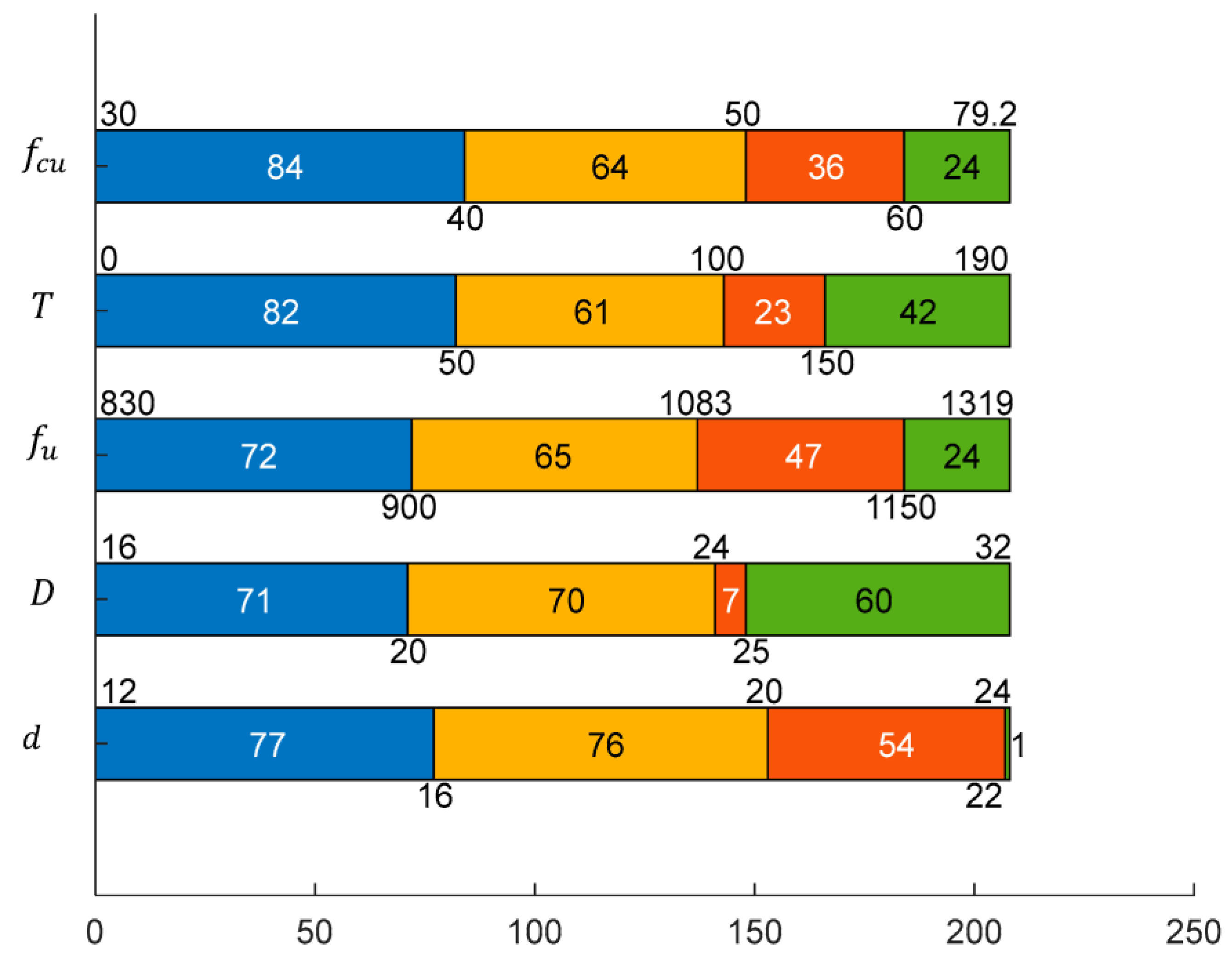
The specific distribution charts of the parameters for the 208 experimental data can be seen in Figure 7. The distribution of most variables in the samples is non-uniform. For example, the bolt diameter primarily ranges from 12 mm to 20 mm, with only one sample having a diameter exceeding 22 mm. The precast hole diameter in the concrete has a main distribution range of 16 mm to 24 mm, with only seven samples having a minimum diameter of 24 mm to 25 mm. The tensile strength of high-strength bolts is mainly distributed between 830 MPa and 1083 MPa. The main distribution range of pretension force is from 0 kN to 100 kN. Additionally, the concrete strength is primarily distributed between 30 MPa and 50 MPa.

4. Model Evaluation

4.1. Existing Evaluation Models

See Table 4. These models have been developed since 2004 and consider both concrete failure and shear connector failure simultaneously.

Table 4. Existing evaluation models.

	Concrete Failure	Connector Fracture	Unit	Model Sequence
EN 1994-1-1 (2004) [25]	$\raisebox{1ex}{$0.29\alpha d^2\sqrt{f_{ck}{E}_c}$}\!\left/ \!\raisebox{-1ex}{${\gamma }_v$}\right.$	$\raisebox{1ex}{$0.8f_u\mathsf{\pi }{d}^2/4$}\!\left/ \!\raisebox{-1ex}{${\gamma }_v$}\right.$	N, mm, MPa	(6)
AISC 360-16 (2016) [31]	$\raisebox{1ex}{$0.5\pi d^2\sqrt{E_c{f}_{ck}}$}\!\left/ \!\raisebox{-1ex}{$4$}\right.$	$\raisebox{1ex}{$\pi d^2{f}_u$}\!\left/ \!\raisebox{-1ex}{$4$}\right.$		(7)
GB 50017 (2017) [32]	$\raisebox{1ex}{$0.43\pi d^2\sqrt{E_c{f}_c}$}\!\left/ \!\raisebox{-1ex}{$4$}\right.$	$\raisebox{1ex}{$0.7\pi d^2{f}_u$}\!\left/ \!\raisebox{-1ex}{$4$}\right.$		(8)
Zhang et al. (2019 [4]	$\raisebox{1ex}{$0.7\pi d^2\sqrt{E_c{f}_{ck}}$}\!\left/ \!\raisebox{-1ex}{$4$}\right.$	$\raisebox{1ex}{$0.62\pi d^2{f}_u$}\!\left/ \!\raisebox{-1ex}{$4$}\right.$		(9)

Table 4. Existing evaluation models.

	Concrete Failure	Connector Fracture	Unit	Model Sequence
EN 1994-1-1 (2004) [25]	$\raisebox{1ex}{$0.29\alpha d^2\sqrt{f_{ck}{E}_c}$}\!\left/ \!\raisebox{-1ex}{${\gamma }_v$}\right.$	$\raisebox{1ex}{$0.8f_u\mathsf{\pi }{d}^2/4$}\!\left/ \!\raisebox{-1ex}{${\gamma }_v$}\right.$	N, mm, MPa	(6)
AISC 360-16 (2016) [31]	$\raisebox{1ex}{$0.5\pi d^2\sqrt{E_c{f}_{ck}}$}\!\left/ \!\raisebox{-1ex}{$4$}\right.$	$\raisebox{1ex}{$\pi d^2{f}_u$}\!\left/ \!\raisebox{-1ex}{$4$}\right.$		(7)
GB 50017 (2017) [32]	$\raisebox{1ex}{$0.43\pi d^2\sqrt{E_c{f}_c}$}\!\left/ \!\raisebox{-1ex}{$4$}\right.$	$\raisebox{1ex}{$0.7\pi d^2{f}_u$}\!\left/ \!\raisebox{-1ex}{$4$}\right.$		(8)
Zhang et al. (2019 [4]	$\raisebox{1ex}{$0.7\pi d^2\sqrt{E_c{f}_{ck}}$}\!\left/ \!\raisebox{-1ex}{$4$}\right.$	$\raisebox{1ex}{$0.62\pi d^2{f}_u$}\!\left/ \!\raisebox{-1ex}{$4$}\right.$		(9)

All models share the same form as Equation (6), with only variations in coefficients. The models take into account variables such as the elastic modulus of concrete, compressive strength of concrete, tensile strength of shear connectors, and bolt diameter. According to Formulas (2) and (3), mentioned in Ding et al. [17], $E_c$ and $f_{ck}$ can be related to the compressive strength of standard concrete cubes. Additionally, considering the prediction of the ultimate strength of HSFGB shear connectors, the influences of preformed hole diameter in concrete and bolt pretension force are also important. Hence, the variables taken into consideration in this study are deemed viable.

4.2. Model Assessment

To assess the models presented in Table 4, it is recommended to evaluate them based on both the average value and the coefficient of variation (COV) of the obtained results. The average value provides a comprehensive measure of the deviation between the calculated values and the experimental values. A significantly higher average value suggests an overestimation of shear strength, while a considerably lower average value indicates a more conservative approach. The coefficient of variation is used to assess the dispersion between the calculated values and the experimental values. A lower coefficient of variation, approaching zero, indicates reduced dispersion and a more precise model.

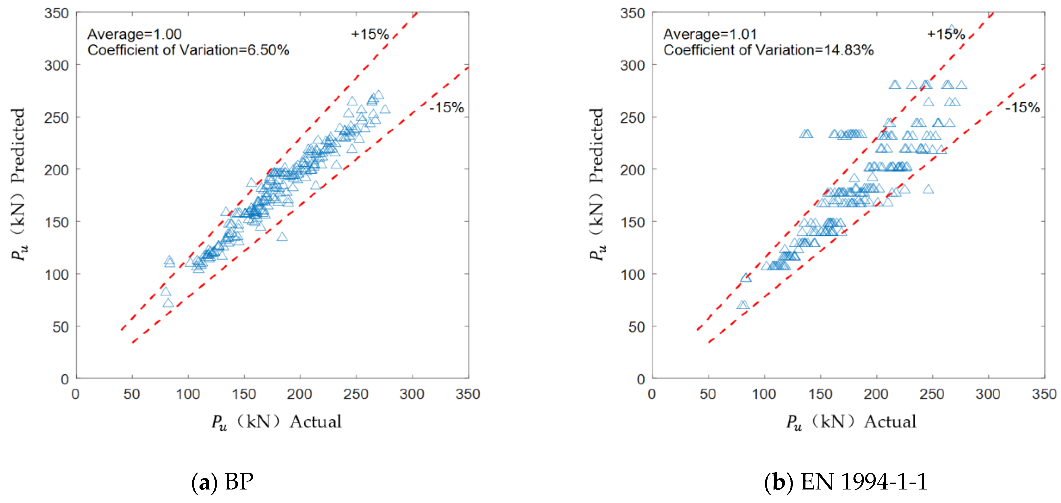
Figure 8 presents a statistical analysis of the collected data, comparing the calculated values and the actual values of the models proposed in different literature sources. This analysis highlights the disparities between the proposed models and the observed outcomes. For the models proposed by AISC 360-16 (2016) and GB 50017 (2017), the average ratio between the predicted values and the actual values is 0.91 and 0.76, respectively. These models exhibit overly conservative predictions for the shear-carrying capacity of the specimens. On the other hand, the models proposed by EN 1994-1-1 (2004) and Zhang et al. (2019) have average ratios of 1.01 and 0.99, respectively, indicating higher accuracy. EN 1994-1-1 (2004) has the lowest COV value at only 14.83%.

5. Establishment of the Data-Driven Model

As stated in Section 4, the research findings suggest that the coefficient of variation for the ratio between the calculated values and the experimental values falls within the range of 14% to 18.5%. Additionally, it is proposed that further analysis should be conducted to validate these results. Building upon this, our objective in this section is to develop a data-driven machine learning model for predicting the ultimate strength of HSFGB shear connectors in composite beams. By adopting this approach, we aim to obtain a more precise and reliable prediction model for the ultimate strength of HSFGB shear connectors.

5.1. Model Construction and Evaluation

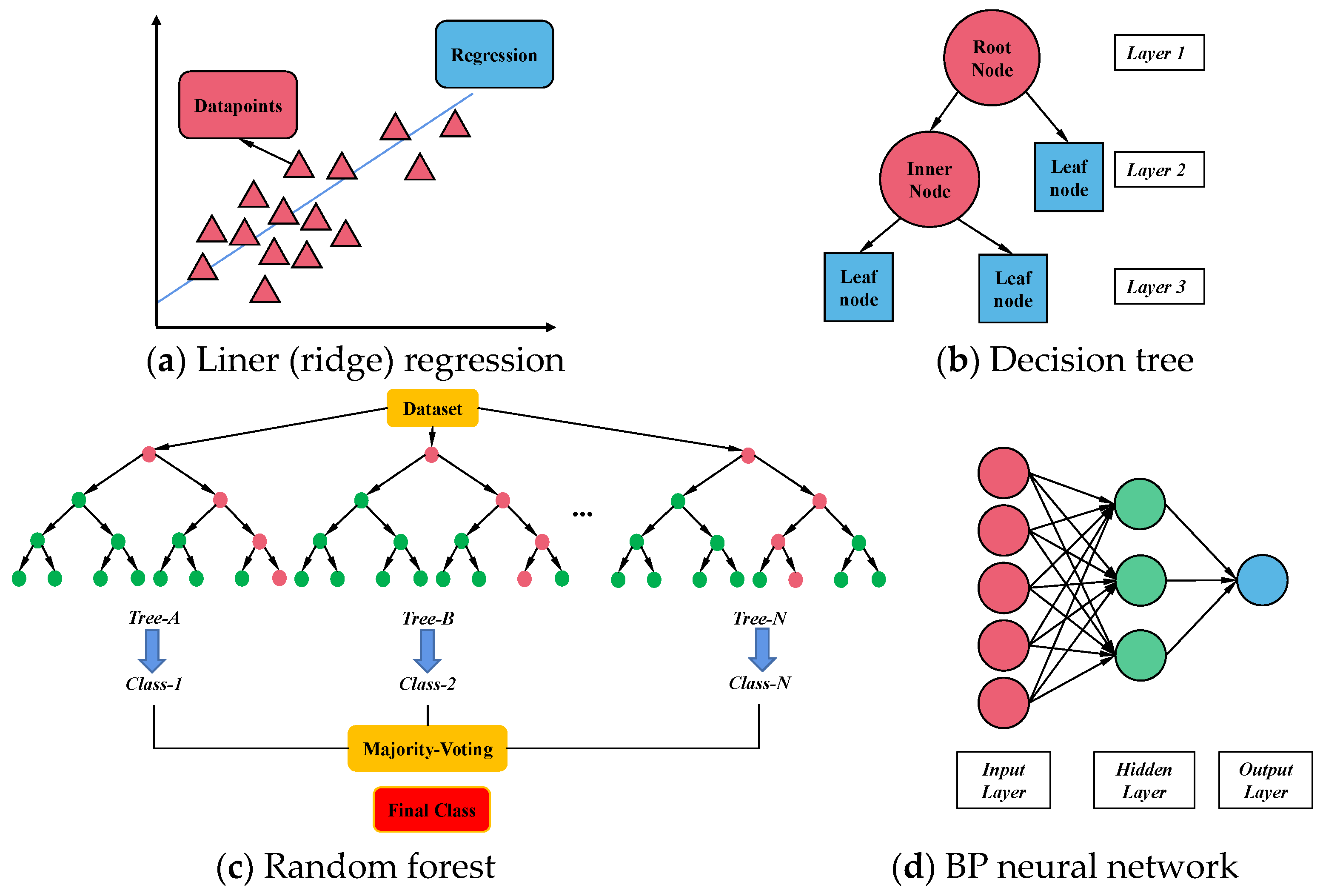
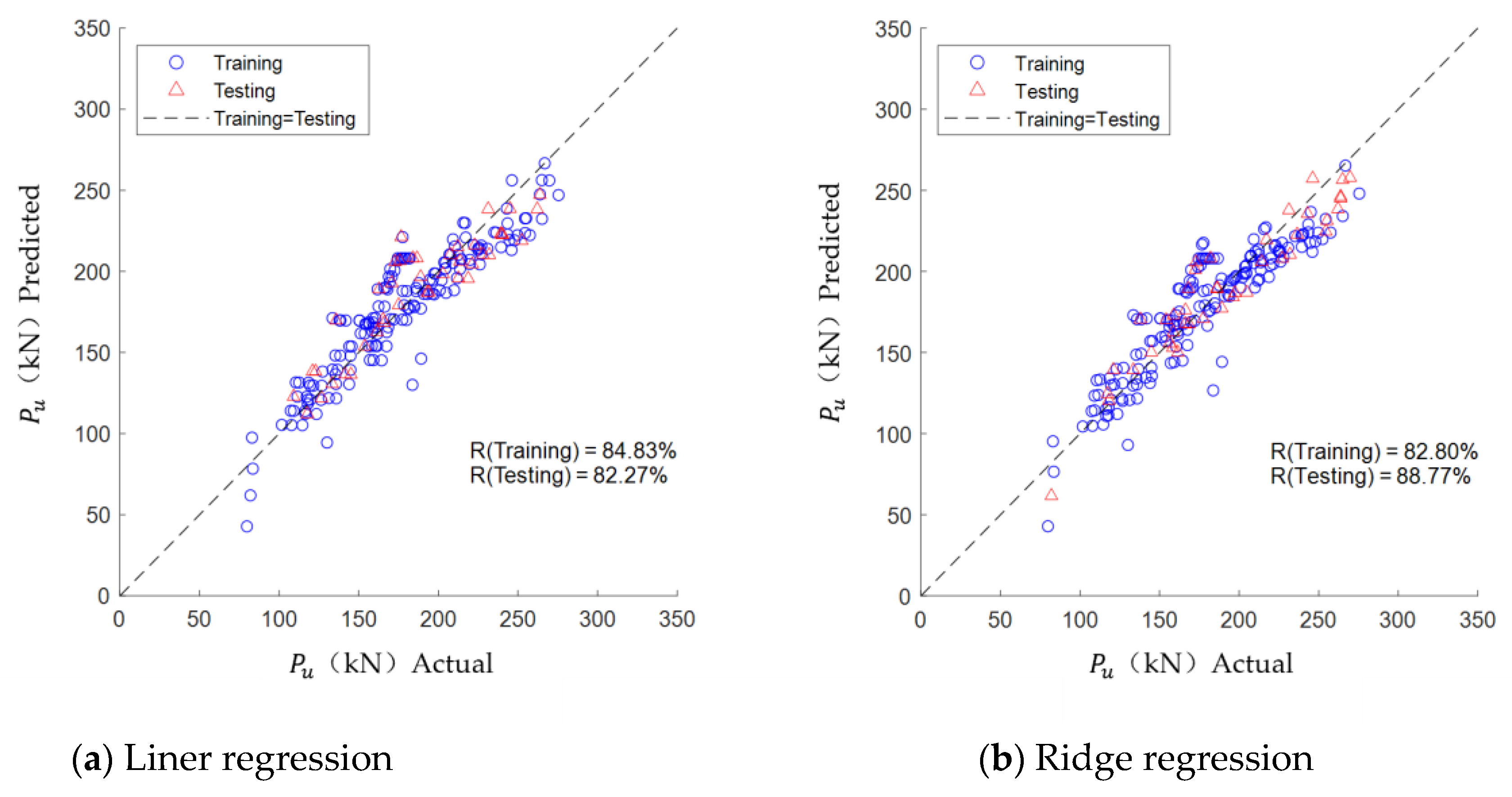
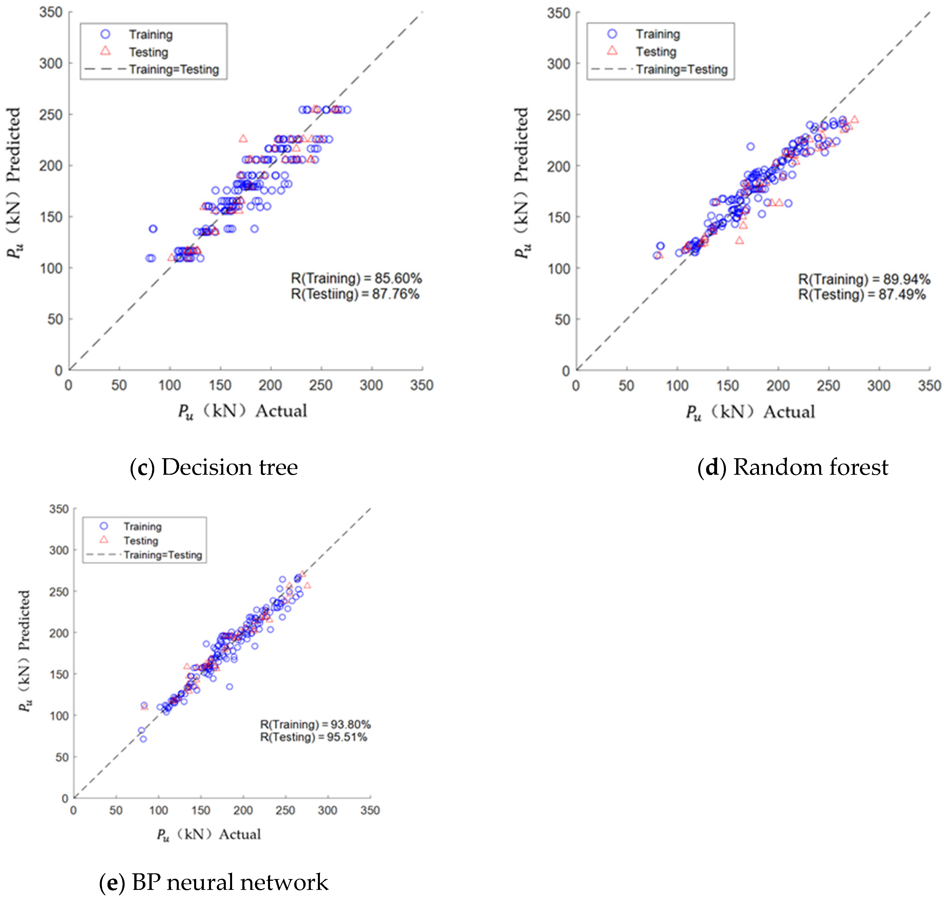
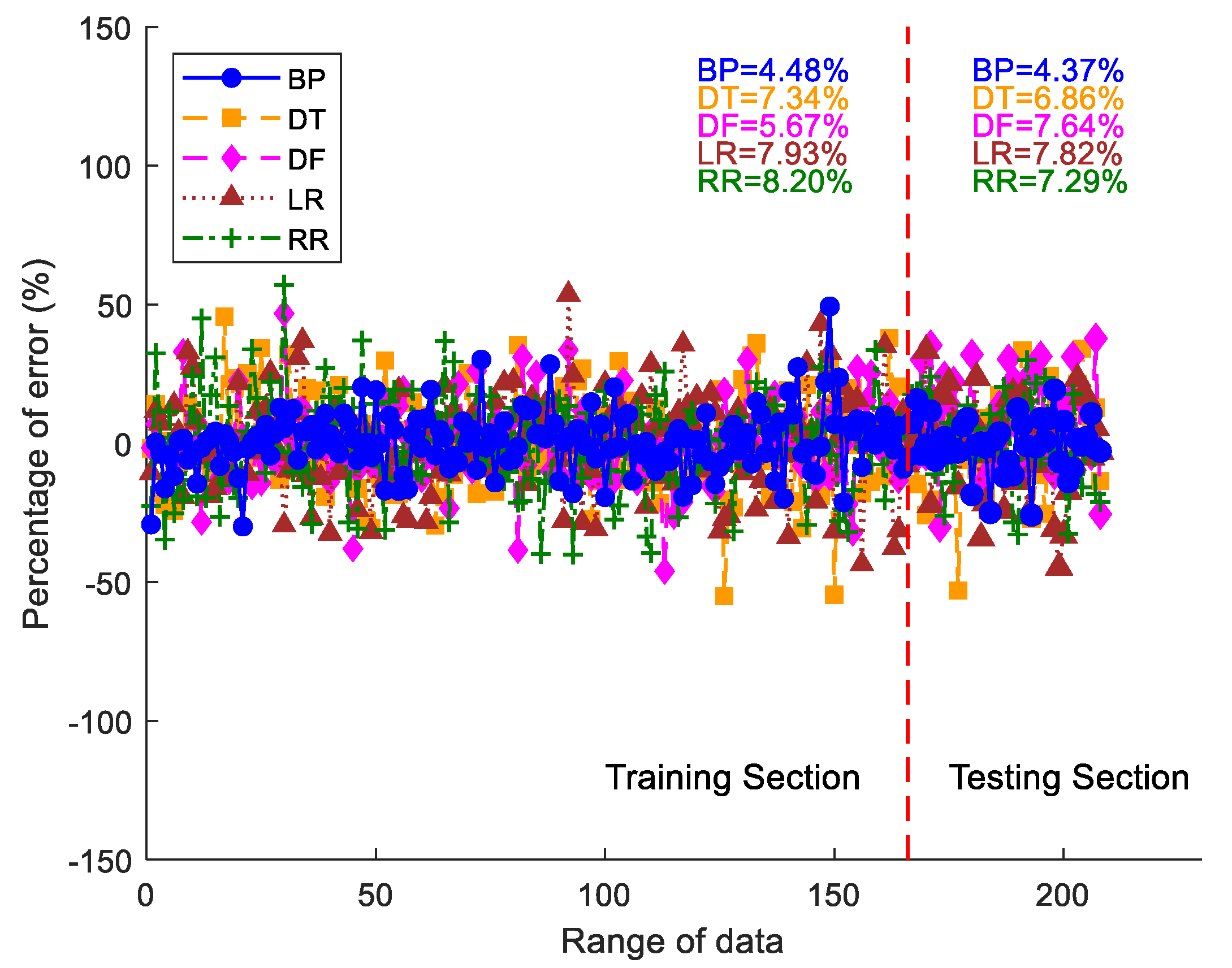
The machine learning model integrates established linear and nonlinear models. Linear regression and ridge regression are employed as the linear models, while decision trees, random forests, and backpropagation neural networks are utilized as the nonlinear models (refer to Figure 9). The dataset used for the model consists of 208 data points from experiments conducted by researchers and finite element analyses (see Table 1). The model is trained using 80% of randomly partitioned data, and the remaining 20% is used for testing. The input variables include bolt diameter, preformed hole diameter in concrete, high-strength bolt tensile strength, preload force, and concrete strength. The output variable is the shear-bearing capacity. The model’s performance is evaluated using the following two metrics: the coefficient of determination (R-squared) and the mean absolute percentage error. Figure 10 and Figure 11 depict the visual representation of the coefficient of determination and the mean absolute percentage error of the model, respectively.

The BP neural network model outperforms the LR, RR, DT, and RF models in terms of coefficient of determination for both the training and testing sets, exceeding 90% in both cases.

By analyzing Figure 11, it can be noted that the LR and DT models display low percentage errors for both the training and testing sets, with values of 0.11% and 0.48%, respectively. On the other hand, the RR and RF models exhibit notably different percentage errors between the training and testing sets, with values of 0.91% and 1.97%, respectively. In contrast, the BP neural network model demonstrates percentage errors that not only have closer values between the training and testing sets but are also considerably lower at 4.48% and 4.37%, respectively.

In summary, the BP neural network model outperforms other models by achieving the highest coefficient of determination and the lowest percentage error. Therefore, it is considered the most suitable model for predicting the ultimate strength of HSFGB shear connectors. Furthermore, when compared to other well-established models (as shown in Figure 12), the BP neural network model demonstrates a lower coefficient of variation than the model defined in EN 1994-1-1 (2004).

5.2. Research on Variables in Studies

5.2.1. Analysis of the Importance of Research Variables

In this section, an analysis of importance is conducted to investigate the significant factors that influence the ultimate strength of HSFGB shear connectors in composite beams. The mean impact value (MIV) is commonly used to extract the feature importance of the BP neural network. The MIV algorithm is primarily employed to detect which input variables have an impact on the output and is a method used for variable selection and assessing variable importance. The MIV calculation formula is shown in Equation (6). Two sets of data are obtained by reducing and increasing the value of a particular input variable by 10% while keeping other input variables unchanged.

$$MIV=\frac{1}{n}{\sum }_{i=1}^n(y_{up}^{\left(i\right)}-y_{down}^{\left(i\right)})$$

(10)

where:

• $y_{up}^{\left(i\right)}$: The predicted value for the $i$-th sample after increasing the variable by 10%;
• $y_{down}^{\left(i\right)}$: The predicted value for the $i$-th sample after decreasing the variable by 10%.

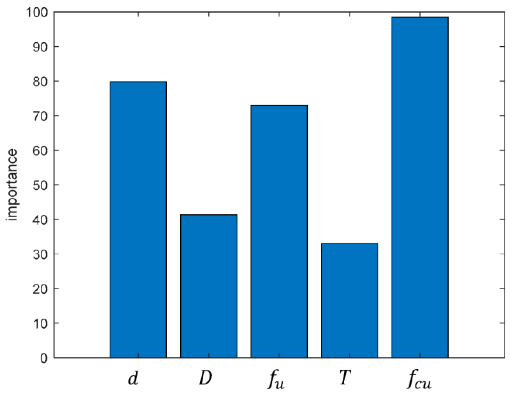
The variable importance results after calculations can be seen in Figure 13.

From Figure 13, it can be observed that the importance of variables for the shear connection joint ultimate strength is in the following order: concrete strength, bolt diameter, bolt ultimate tensile strength, preformed hole diameter in concrete, and bolt preload.

5.2.2. Analysis of the Sensitivity of Research Variables

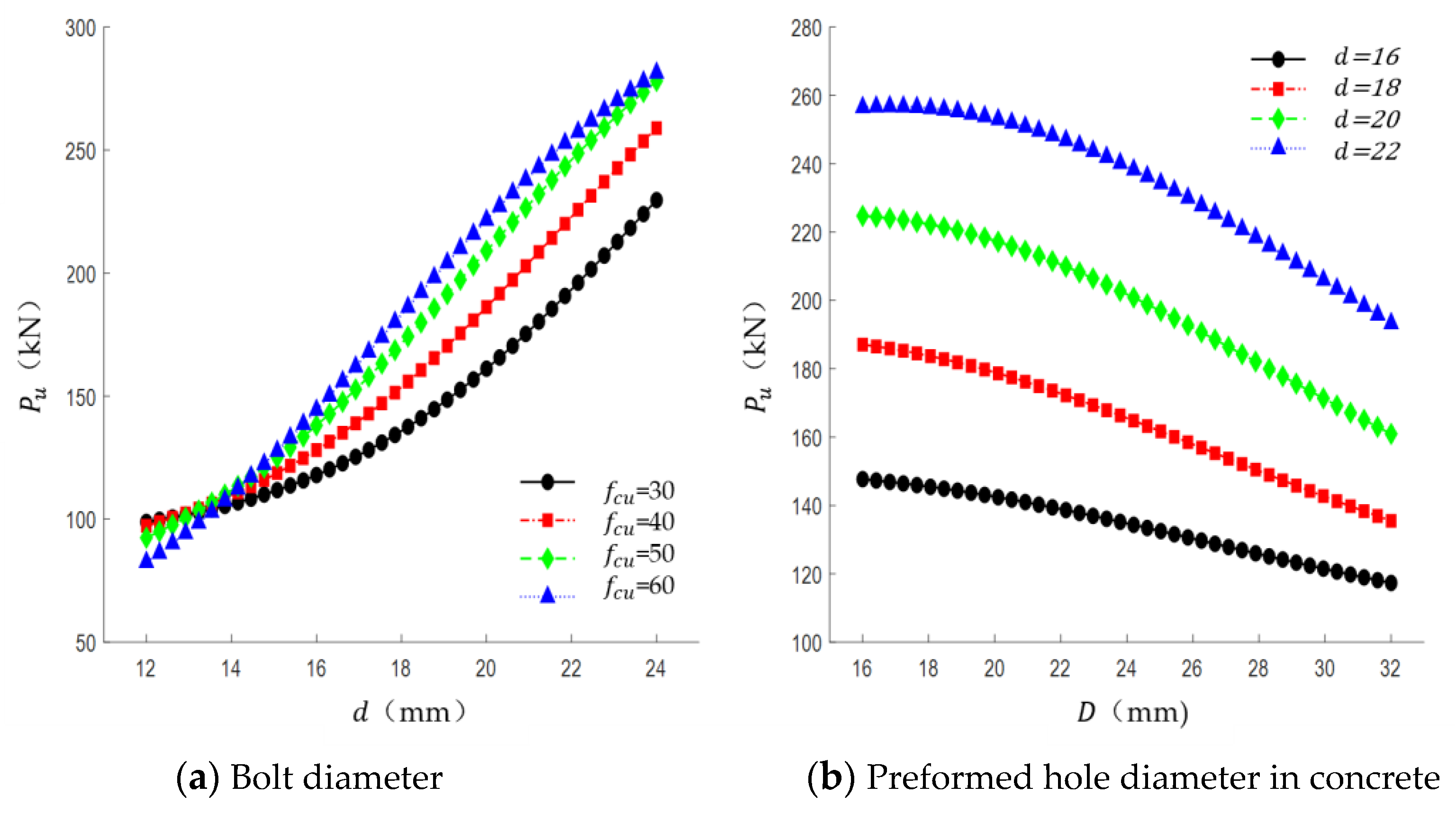
To investigate the correlation between different individual variables and the ultimate strength, we conducted a comprehensive sensitivity analysis. The analysis was performed using the BP neural network model. The variable values are held constant while the variable is varied across four different levels: $d$ = 16, 18, 20, and 22 (with $f_{cu}$ taking values of 30, 40, 50, and 60 when studying $d$). The variable values are obtained from the average values of 208 sets of data collected from Table 1, respectively: $D$ = 23.3 mm, $f_u$ = 1019.4 MPa, $T$= 81.5 kN, $f_{cu}$ = 48 GPa. The relationship between each variable and the ultimate strength of HSFGB shear connectors is shown in Figure 14.

From Figure 14a, it is apparent that the ultimate strength of HSFGB shear connectors demonstrates a direct correlation with the bolt diameter. This relationship is observed across various concrete strengths. Notably, the growth rate of ultimate strength becomes more pronounced for bolt diameters exceeding 14 mm.

From Figure 14b, it can be seen that at different bolt diameters, the ultimate strength of HSFGB shear connectors is inversely proportional to the preformed hole diameter in concrete.

From Figure 14c, it can be observed that the ultimate strength of HSFGB shear connectors is directly proportional to their ultimate strength.

From Figure 14d, it can be seen that at different bolt diameters, the ultimate strength of HSFGB shear connectors exhibits a steady increase with the increase in bolt pretension until it reaches a plateau. However, when the bolt pretension exceeds 130 kN, the ultimate strength starts to rise again before eventually stabilizing.

From Figure 14e, it can be observed that at bolt diameters of 18, 22, and 24, the ultimate strength of HSFGB shear connectors shows an initial increase followed by a decrease with the increase in concrete strength. When utilizing an HSFGB shear connector with a bolt diameter of 16 mm, the ultimate load capacity exhibits a direct proportionality to the strength of the concrete.

5.3. Formulation Development

Formulas in the BP neural network rely on carefully determined interlayer weights and thresholds, which determine the network’s behavior. Equations (11) and (12) define the transfer functions between layers, reflecting information processing and the network’s output. Precise interlayer connection weights and biases can be found in Table 3, guiding the network’s configuration and behavior.

$$tansig\left(\phi \right)=\frac{2}{1+e^{-2\phi }}-1$$

(11)

$$f\left(\phi \right)=\phi$$

(12)

where $\phi =\sum _i{W}_{ij}{x}_i+{\varphi }_j$. In the BP neural network, the connection weight between the i-th layer and the $i$-th neuron is denoted as $W_{ij}$. Additionally, the bias of the $j$-th neuron is represented by ${\varphi }_j$.

Based on

Table 5. Weights for interlayer connections in a neural network.

P			P
			Hidden		Output
		H(1:1)	H(1:2)	H(1:3)	${\mathit{P}}_{\mathit{u}}$
	Bias	2.864	−1.5351	6.0514
	$d$	−0.1355	0.0233	−0.1857
	$D$	0.0537	0.085	−0.1541
Input	$f_u$	−0.0003	0.0016	−0.0048
	$T$	0.0027	0.0066	0.057
	$f_{cu}$	−0.0261	−0.0433	−0.0664
	Bias				182.0298
	H(1:1)				−134.64
Hidden	H(1:2)				78.9768
	H(1:3)				33.4263

, we can obtain Equation (13) to predict the ultimate strength ($P_u$ in kN) of HSFGB shear connectors in composite beams by considering the following problem variables: bolt diameter ($d$ in mm), concrete borehole diameter ($D$ in mm), high-strength bolt ultimate tensile strength ($f_u$ in MPa), bolt pretension force ($T$ in mm), and concrete compressive strength ($f_{cu}$ in MPa). Please note that the provided equation is applicable only within the range of the input variables. In this study, we strive to incorporate practical requirements by considering the various ranges of different variables. The provided formula represents the model expression obtained after extracting the BP neural network. It has been verified that the maximum error between the predicted values of the model expression and the BP neural network is only $1.7053\times {10}^{-13}$. The error is attributed to the precision of the extracted coefficients being controlled to only four significant figures after the decimal point. The applicable parameter range is as follows: $d$ (12~24 mm), $D$ (16~32 mm) $f_u$ (830~1319 Mpa), $T$ (0~190 kN), $f_{cu}$ (30~79.2 Mpa).

$$P_u=\frac{-269.279}{1+e^{-2{\beta }_1}}+\frac{157.9536}{1+e^{-2{\beta }_2}}+\frac{66.8526}{1+e^{-2{\beta }_3}}+204.2662$$

(13)

$$\begin{gathered} {\beta }_1=-0.13546d+0.053719D-0.00033762f_u \\ +0.0026984T-0.026075f_{cu}+2.864 \end{gathered}$$

(14)

$$\begin{gathered} {\beta }_2=0.023253d+0.085009D+0.0016156f_u \\ +0.0065562T-0.043332f_{cu}-1.5351 \end{gathered}$$

(15)

$$\begin{array}{l}{\beta }_3=-0.18569d-0.15407D-0.004812f_u+0.05698T-\\ 0.066369f_{cu}+6.0514\end{array}$$

(16)

6. Conclusions

This research develops practical formulas to predict the ultimate strength of HSFGB shear connectors in composite beams. Finite element analyses and variable studies are used to simulate and validate the behavior of these connectors. The findings contribute to accurate formulas considering connector characteristics for engineering design and analysis. Overall, the research successfully predicts the ultimate strength of HSFGB shear connectors.

By analyzing researchers’ experimental data and a large amount of finite element data, five data-driven models were evaluated, including ridge regression, least squares, decision trees, random forests, and BP neural networks. Among these models, the BP neural network exhibited the highest accuracy on the dataset and was, therefore, selected for further analysis.

An analysis of variable importance indicated that the concrete strength, bolt diameter, and bolt tensile strength significantly influenced the ultimate strength of the shear connector. In a sensitivity analysis, we observed that, with the exception of concrete strength and bolt pretension, the other variables exhibited either a positive or negative correlation with compressive strength.

Based on these findings, we proposed a more accurate prediction formula for the ultimate strength of HSFGB shear connectors. It is important to note that the proposed relationships are only applicable within the range of data used in this study and can be utilized by engineers during relevant design processes.

The method used in this article is the traditional BP neural network, and the collected data are also limited. To establish a better model, it is necessary to incorporate more deep learning models and gather a larger amount of data.

References

1. Marshall, W.T.; Nelson, H.M.; Banerjee, H.K. An experimental study of the use of high-strength friction-grip bolts as shear connectors in composite beams. J. Struct. Eng. 1971, 49, 171–178. [Google Scholar]
2. Kwon, G.; Engelhardt, M.D.; Klingner, R.E. Behavior of post-installed shear connectors under static and fatigue loading. J. Constr. Steel Res. 2010, 66, 532–541. [Google Scholar] [CrossRef]
3. Pathirana, S.W.; Uy, B.; Mirza, O.; Zhu, X. Flexural behaviour of composite steel-concrete beams utilizing blind bolt shear connectors. Eng. Struct. 2016, 114, 181–194. [Google Scholar] [CrossRef]
4. Zhang, Y.; Chen, B.; Liu, A.; Pi, Y.-L.; Zhang, J.; Wang, Y.; Zhong, L. Experimental study on shear behavior of high strength bolt connection in prefabricated steel-concrete composite beam. Compos. Part B Eng. 2019, 159, 481–489. [Google Scholar] [CrossRef]
5. Naderpour, H.; Mirrashid, M.; Parsa, P. Failure mode prediction of reinforced concrete columns using machine learning methods. Eng. Struct. 2021, 248, 113263. [Google Scholar] [CrossRef]
6. Zhang, F.; Wang, C.; Liu, J.; Zou, X.; Sneed, L.H.; Bao, Y.; Wang, L. Prediction of FRP-concrete interfacial bond strength based on machine learning. Eng. Struct. 2023, 274, 115156. [Google Scholar] [CrossRef]
7. Vu, Q.-V.; Truong, V.-H.; Thai, H.-T. Machine learning-based prediction of CFST columns using gradient tree boosting algorithm. Compos. Struct. 2020, 259, 113505. [Google Scholar] [CrossRef]
8. Hu, T.; Zhang, H.; Zhou, J. Prediction of the Debonding Failure of Beams Strengthened with FRP through Machine Learning Models. Buildings 2023, 13, 608. [Google Scholar] [CrossRef]
9. Huang, L.; Chen, J.; Tan, X. BP-ANN based bond strength prediction for FRP reinforced concrete at high temperature. Eng. Struct. 2022, 257, 114026. [Google Scholar] [CrossRef]
10. Li, H.; Yang, D.; Hu, T. Data-Driven Model for Predicting the Compressive Strengths of GFRP-Confined Reinforced Concrete Columns. Buildings 2023, 13, 1309. [Google Scholar] [CrossRef]
11. Nguyen, H.; Vu, T.; Vo, T.P.; Thai, H.-T. Efficient machine learning models for prediction of concrete strengths. Constr. Build. Mater. 2020, 266, 120950. [Google Scholar] [CrossRef]
12. Tohidi, S.; Sharifi, Y. Load-carrying capacity of locally corroded steel plate girder ends using artificial neural network. Thin-Walled Struct. 2016, 100, 48–61. [Google Scholar] [CrossRef]
13. Bagherzadeh, F.; Shafighfard, T.; Khan, R.M.A.; Szczuko, P.; Mieloszyk, M. Prediction of Maximum Tensile Stress in Plain-Weave Composite Laminates with Interacting Holes via Stacked Machine Learning Algorithms: A Comparative Study. Mech. Syst. Signal Process. 2023, 195, 110315. [Google Scholar] [CrossRef]
14. Asgarkhani, N.; Kazemi, F.; Jankowski, R. Machine Learning-Based Prediction of Residural Drift and Seismic Risk Assessment of Steel Moment-Resisting Frames Considering Soil-Structure Interaction. Comput. Struct. 2023, 289, 107181. [Google Scholar] [CrossRef]
15. Sharifi, Y.; Moghbeli, A.; Hosseinpour, M.; Sharifi, H. Study of Neural Network Models for the Ultimate Capacities of Cellular Steel Beams. Iran. J. Sci. Technol. Trans. Civ. Eng. 2019, 44, 579–589. [Google Scholar] [CrossRef]
16. Sarothi, S.Z.; Ahmed, K.S.; Khan, N.I.; Ahmed, A.; Nehdi, M.L. Predicting bearing capacity of double shear bolted connections using machine learning. Eng. Struct. 2021, 251, 113497. [Google Scholar] [CrossRef]
17. Hosseinpour, M.; Daei, M.; Zeynalian, M.; Ataei, A. Neural networks-based formulation for predicting ultimate strength of bolted shear connectors in composite cold-formed steel beams. Eng. Appl. Artif. Intell. 2023, 118, 105614. [Google Scholar] [CrossRef]
18. Xing, Y.; Liu, Y.; Shi, C.; Wang, Z.; Guo, Q.; Jiao, J. Static behavior of high strength friction-grip bolt shear connectors in composite beams. Steel Compos. Struct. 2022, 42, 407–426. [Google Scholar] [CrossRef]
19. Khan, R.M.A.; Shafighfard, T.; Ali, H.Q.; Mieloszyk, M.; Yildiz, M. Strength Prediction and Experimental Damage Investigations of Plain Woven CFRPs with Interacting Holes Using Mul-ti-Instrument Measurements. Polym. Compos. 2023, 44, 3594–3609. [Google Scholar] [CrossRef]
20. Ding, F.; Ying, X.; Zhou, L.; Yu, Z. Unified calculation method and its application in determining the uniaxial mechanical properties of concrete. Front. Arch. Civ. Eng. China 2011, 5, 381–393. [Google Scholar] [CrossRef]
21. Loh, H.; Uy, B.; Bradford, M. The effects of partial shear connection in composite flush end plate joints Part II—Analytical study and design appraisal. J. Constr. Steel Res. 2005, 62, 391–412. [Google Scholar] [CrossRef]
22. Shi, G.; Shi, Y.; Wang, Y.; Bradford, M.A. Numerical simulation of steel pretensioned bolted end-plate connections of different types and details. Eng. Struct. 2008, 30, 2677–2686. [Google Scholar] [CrossRef]
23. Rabbat, B.G.; Russell, H.G. Friction Coefficient of Steel on Concrete or Grout. J. Struct. Eng. 1985, 111, 505–515. [Google Scholar] [CrossRef]
24. Guo, Q.; Chen, Q.-W.; Xing, Y.; Xu, Y.-N.; Zhu, Y. Experimental Study of Friction Resistance between Steel and Concrete in Prefabricated Composite Beam with High-Strength Frictional Bolt. Adv. Mater. Sci. Eng. 2020, 2020, 1292513. [Google Scholar] [CrossRef]
25. EN 1994-1-1; Eurocode 4: Design of Composite Steel and Concrete Structures-Part 1-1: General Rules and Rules for Buildings. European Committee for Standardizaton: Brussels, Belgium, 2004.
26. GB 50010-2010; Code for Design of Concrete Structures. Ministry of Housing and Urban-Rural Development of the People’s Republic of China: Beijing, China, 2015.
27. Xin, Y. Analysis of compressive strength relationship between concrete cylinder specimen and cube specimen. China Water Power Electrif. 2015, 7, 59–62. [Google Scholar] [CrossRef]
28. Xing, Y.; Yan-Bin, L.; Cai-Jun, S.; Qi, G.; Chen, Q.-W. Experimental Study on Shear Performance of High-Strength Bolted Connections in Restorable Composite Beams. China J. Highw. Transp. 2023, 36, 132–142. [Google Scholar] [CrossRef]
29. Ataei, A.; Zeynalian, M. A study on structural performance of deconstructable bolted shear connectors in composite beams. Structures 2020, 29, 519–533. [Google Scholar] [CrossRef]
30. Zhao, W.; Lu, S.; Jing, X. Shear performance of high-strength bolt connector considering different pad and bolt hole. Structures 2020, 28, 1291–1300. [Google Scholar] [CrossRef]
31. ANSI/AISC 360-16; Specification for Structural Steel Buildings. American Institute of Steel Construction: Chicago, IL, USA, 2016.
32. GB 50017; Code for Design of Steel Structures. Ministry of Housing and Urban-Rural Development of the People’s Republic of China: Beijing, China, 2017.
Figure 1. Typical configuration of the bolted joint.
Buildings 13 02769 g001
Figure 2. Push-out test specimen details (unit: mm).
Buildings 13 02769 g002
Figure 3. Constitutive relationship of high-strength bolts.
Buildings 13 02769 g003
Figure 4. Mesh division.
Buildings 13 02769 g004
Figure 5. 3D view and boundary conditions.
Buildings 13 02769 g005
Figure 6. Failure patterns of the bolts and concrete hole walls for PT1.
Buildings 13 02769 g006
Figure 7. Distributions of the variables.
Buildings 13 02769 g007
Figure 8. Comparisons of the predicted and experimental results [4,25,31,32].
Buildings 13 02769 g008
Figure 9. Architecture of the machine learning model.
Buildings 13 02769 g009
Figure 10. Accuracy of the machine learning model’s fit.
Buildings 13 02769 g010aBuildings 13 02769 g010b
Figure 11. Error percentage of the machine learning models.
Buildings 13 02769 g011
Figure 12. Model performance of BP and EN 1994-1-1 (2004) [25].
Buildings 13 02769 g012
Figure 13. Analysis of the importance of research variables.
Buildings 13 02769 g013
Figure 14. Sensitivity analysis of research variables.
Buildings 13 02769 g014aBuildings 13 02769 g014b